Vortex beam generation with variable topological charge based on a spiral slit
-
Han Wang

 and
Yangjian Cai
and
Yangjian Cai

Abstract
We propose a vortex beam generator based on a nanometer spiral slit and explore the propagation rule of the topological charge. Compared to the common methods of generation of a vortex beam with a fixed topological charge, the optical vortex generated by the proposed vortex beam generator has the topological charge varying with the propagation distance. The value of topological charge can be modulated by the geometric charge of the spiral slit and the propagation distance. Theoretical analysis predicts the variation rule of the topological charge of vortex beam in the near field, and numerical simulations and experimental measurement verify the proposed scheme. Discussion on the shape and structure of the spiral slit is also presented. This work provides the theoretical foundation for the generation of a vortex field with variable topological charge. The simple geometry of the vortex beam generator and the flexible modulation of the topological charge must inspire applications of the vortex beam.
1 Introduction
A vortex beam refers to a light beam possessing a helical phase front and can be described by a transverse phase structure exp(ilφ), with φ denoting the azimuthal angle and l representing the topological charge (TC) of the optical field [1]. TC of the vortex field may be an integer or a fraction. Since vortex beams carry orbital angular momentum (OAM) of lħ [2], they have numerous applications in optical micromanipulation [3], free-space communication [4], material processing [5], and digital imaging [6].
The common methods to generate vortex beams include a spiral phase plate [7], a spatial light modulator [8], a cylindrical lens [9], and a metasurface [10]. As is known, a vortex beam generated by any of the common methods carries a fixed OAM during the propagation. Recently, a vortex beam with controllable TC during its propagation has attracted much attention. The use of frozen waves realizes the control of the TC of the beam along the propagation direction [11]. The special Fermat spiral enables the local TC to vary during propagation over large distances [12]. The biaxial Laguerre–Gaussian (LG) beam may adjust conveniently the fractional TC of a vortex beam [13]. Studies have predicted longitudinal control of the OAM, yet more physical problems such as the theoretical basis of controllable TC and the dependence of TC on the structure, propagation, and illuminating light have not been explored to date.
In this work, we study essentially the propagation of the vortex beam generated by a nanometer spiral slit etched on a metal film and explore the evolution of the TC with increase in the propagation distance. Theoretical analysis provides the expression of the phase front as a function of the propagation distance, chirality of the incident polarization light, and the rotation direction of the spiral slit. Then the spatial position for a certain TC can be ascertained. Numerical simulations and practical experiment validate the rule governing the variation of TC with the propagation distance. The influence of the shape and structure of spiral slits on the formation of TC is also discussed. This new study on the vortex beam with variable TC is expected to expand flexible applications of the vortex beam to many fields including optical manipulation, microscopy imaging, and quantum information processing [14], [15].
2 Design principle of the vortex beam generator
We choose an Archimedes spiral slit etched on a silver film as the elementary diffraction system to study the generation of the vortex beam. The orbit of a nanometer spiral slit can be expressed in polar coordinates as [16]
where r and φ are the radial and angular coordinates of the spiral slit, r0 is the initial radius, l is an integer representing the geometric charge, and λ is the illumination wavelength. When lλ is much smaller than r0, we can write the above equation as r2=r02+lλr0φ/π by neglecting the term (lλφ/2π)2, which is just the expression for a Fermat spiral.
When a plane wave propagating along the z-axis transits the nanometer spiral slit of width w from the glass substrate, as shown in Figure 1, a vortex beam can be generated in near field immediately after the spiral slit, as described in a previous work [17], [18], and the TC is taken as a constant l ± 1, with the positive and negative signs corresponding to the left-handed circularly polarized (LCP) and right-handed circularly polarized (RCP) light, respectively [19], [20]. As a matter of fact, the vortex beam generated by the spiral slit is relevant to the propagation distance, and the value of TC decreases with increase in the propagation distance, as shown in the inserted patterns in Figure 1. This variation of the TC with the propagation distance is just the focus of this paper, and the following section gives a detailed theoretical analysis.

Schematic diagram of the propagation of the optical vortex generated by a nanometer spiral slit.
3 Theoretical analysis
According to the scalar diffraction theory, the transmission field of a metal spiral slit at distance z away from the object plane can be approximately written as
where u(x0, y0) is the amplitude of the transmission field immediately after the spiral slit, and cos θ=z/ρ denotes the inclination factor, with ρ=[(x–x0)2+(y – y0)2+z2]1/2 representing the distance from the object point to the observation point.
For an observation point along the propagation axis, ρ in Eq. (2) can be simplified by ρ=[(r0+lλφ/2π)2+z2]1/2. Since the phase difference from two adjacent object points to an observation point and their distance difference has the relationship dα=2πdρ/λ=l(r0+lλφ/2π)dφ/(r02+z2)1/2, after the integration, the phase of the light field around the observation point can be approximated by
In fact, 2π should be added or subtracted to the phase when the incident light is circularly polarized.Thus, the TC of the vortex field with LCP and RCP light illumination should be
This expression gives the dependence of the TC of the vortex field on the geometric charge l of spiral slit, the initial radius r0 of the spiral slit, and the propagation distance z. It is easy to see that TC at large propagation distances is smaller and also that it changes with the initial radius and the illuminating wavelength. Moreover, TC for LCP light illumination is always 2 larger than that for RCP light illumination.
On the basis of Eq. (2), with a spiral slit and the illumination condition set, the longitudinal and transverse field distributions transmitted through the spiral slit can be obtained. Since the central intensity of the optical vortex is always equal to zero, the positions of the optical vortex can be ascertained according to the extreme intensities at the propagation axis, and the TC of the vortex field can be extracted from the transverse field distribution at these positions.
Figure 2 gives the diffraction distributions of an Archimedes spiral slit calculated on the basis of Eq. (2), where Figure 2A–D is for LCP light illumination and Figure 2E–H is for RCP light illumination. The initial radius of the spiral slit is r0=6 μm, the geometric charge is l=4, and the illuminating wavelength is 0.633 μm. Figure 2A and E shows the intensity distributions of the spiral slit along the longitudinal direction. For observing simultaneously the phase distribution, the transverse diffraction distributions in Figure 2B–D and 2F–H are the real parts of the diffraction fields. The longitudinal propagation distance takes values in the range [0.5 μm, 35 μm]. The propagation distances for the transverse diffraction patterns are chosen as z=1.5, 6.3, and 12.3 μm, where the axial intensities at these positions are close to zero. From the results of Figure 2, we can see that the longitudinal and transverse distributions change with the propagation distance. The TCs extracted from the transverse distributions are 5, 4, and 3 for LCP light illumination and 3, 2, and 1 for RCP light illumination, which can be seen clearly from the bright and dark changes in the red circles. The positions of the vortex field with integral TC can be approximately ascertained based on Eq. (4), and the corresponding results are consistent with the extracted theoretical ones shown in Figure 2.

Theoretic results for field distributions of spiral slit.
The longitudinal intensity distributions and the real parts of the transverse fields of spiral slit with left-(A–D) and right-handed (E–H) circularly polarized light illumination, where the propagation distance for the transverse diffraction patterns is 1.5, 6.3, and 12.3 μm, respectively.
4 Numerical simulations
In order to verify the variation of TC of the vortex field with the distance of propagation, we perform numerical simulations by using the finite-difference time-domain technique. In practical simulations, perfectly matched layers are used to prevent nonphysical scattering at the boundaries while simulating the transmission of the spiral slit. The thickness of silver film deposited on the glass is 300 nm and the width of the spiral slit is 200 nm. A nonuniform mesh type is used to obtain higher calculation accuracy. A plane wave of wavelength of 0.633 μm illuminates the sample from the glass substrate. The dielectric constant of silver is taken from Palik [21].
Figure 3 shows the longitudinal and transverse diffraction distributions of the spiral slit, with the initial radius of spiral slit r0=6 μm and the geometric charge l=4. Figure 3A–D gives the results with LCP light illumination, where the propagation distance for longitudinal intensity distributions is limited to within the range [0.5 μm, 35 μm], and the positions of the transverse phase distributions are chosen as z=1.0, 6.4, and 12.2 μm. Figure 3E–H gives the results with RCP light illumination, where the propagation distance for longitudinal intensity distribution is also limited within [0.5 μm, 35 μm], and the positions of the transverse phase distributions are chosen as z=0.83, 6.2, and 12.6 μm. These transverse fields, except for the case of Figure 3H under RCP light illumination, are extracted at propagation distances with the minimum intensity. Moreover, the transverse intensity distributions are also inserted in the corresponding phase distribution patterns, as shown by the results in the lower right corners of Figure 3B–D and 3F–H. The annular intensity distributions take place at these positions.

Simulation results for field distributions of spiral slit.
The longitudinal intensity and transverse phase distributions of a spiral slit with LCP (A–D) and RCP (E–H) light illumination, where the propagation distance for the transverse phases in (B)–(D) is 1.0, 6.4, and 12.2 μm, and the propagation distance in (F)–(H) is 0.83, 6.2, and 12.6 μm. The inserted patterns in (B–D) and (F–H) are the corresponding intensity distributions.
From the results in Figure 3, we can see that the longitudinal intensity distributions are the same as the theoretical ones shown in Figure 2. The transverse phase distributions show that the TC of the vortex field really decreases with increase in the propagation distance. TC for RCP illumination is always smaller than that for LCP illumination at shorter propagation distances. These rules for the variation of the vortex field are consistent with the theoretical predictions, though the positions of extreme intensities are not completely consistent.
5 Experimental measurement
In order to test further the vortex beam with variable TC, a practical experiment is performed. The experimental setup is depicted in Figure 4A. Linearly polarized light emitted from a He–Ne laser is converted into circularly polarized light by a quarter-wave plate (QWP). Then, the light beam is divided into two equal parts as the object light and the reference light by the beam splitter 1 (BS1). The object light impinges on the sample (S), and its transmission field is magnified by the microscope objective 1 (MO1) and then received by a charge-coupled device (CCD). The reference light is made to interfere with the object light through the beam splitter 2 (BS2) and we test the TC of the optical vortex. A density filter (DF) and the microscope objective 2 (MO2) are used to adjust the intensity of the reference light. For convenience of adjustment, the sample is placed on a moving platform with a precision of 100 nm.
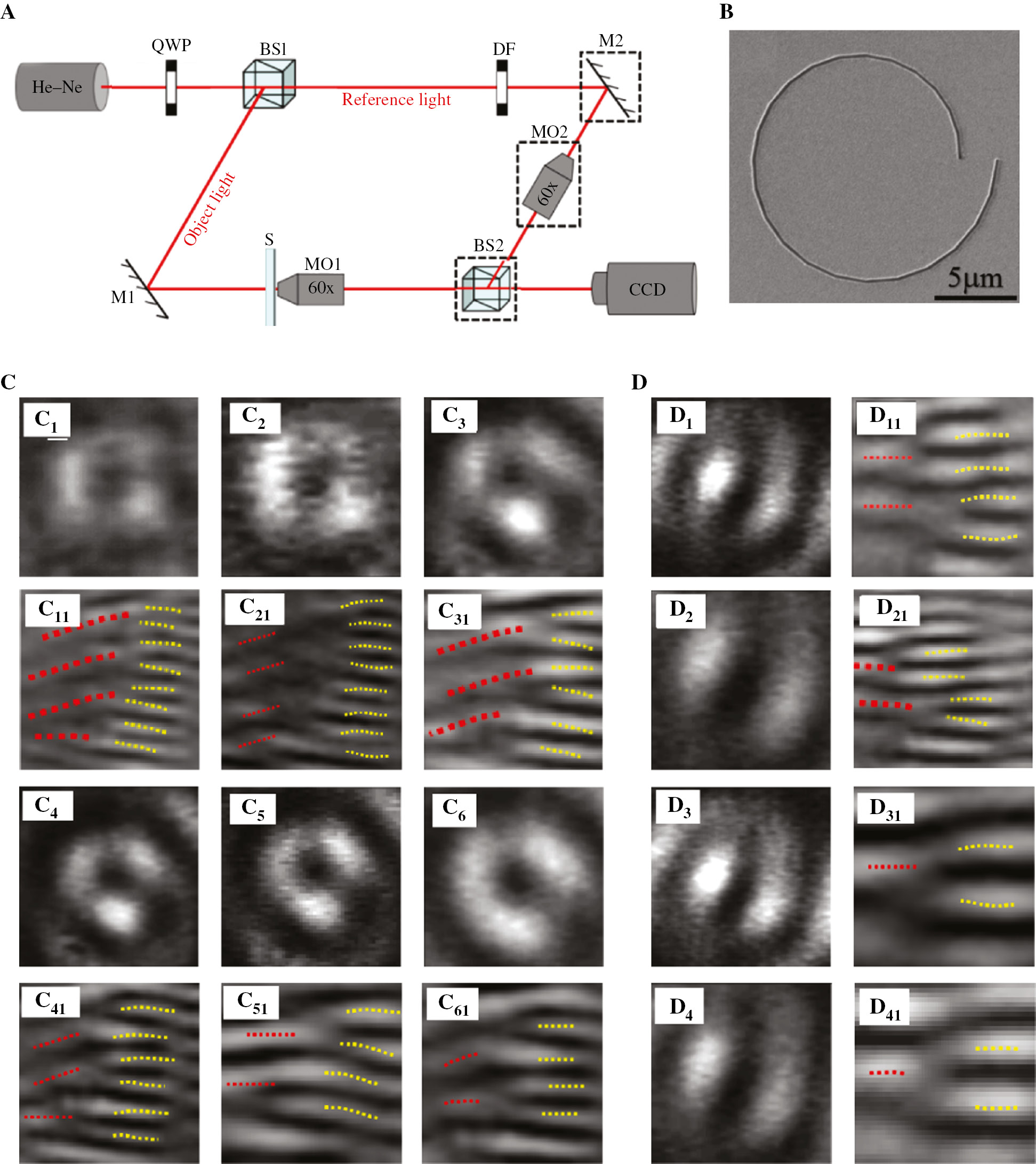
Experiment setup and the measurement results.
(A) Experiment setup. QWP denotes a quarter-wave plate, BS1 and BS2 represent the beam splitters, S is the sample, MO1 and MO2 denote microscope objectives, M1 and M2 are mirrors, and DF is a dense filter. (B) SEM image of the spiral slit. The measured intensity distribution patterns and the interference results in (C) and (D) are for the LCP and RCP light illumination.
We create the vortex beam generator sample according to the design theory. A silver film of thickness 300 nm is deposited on a glass substrate using magnetron sputtering. The sputtering power is 10 W, the vacuum is 7×10⁻⁴ Pa, and the argon partial pressure is 0.5 Pa. Spiral slits of l=4 with width and initial radius of 200 nm and 6 μm are fabricated by focused ion beam etching, where the voltage is 30 kV and the current is 92 pA. Figure 4B shows the scanning electron microscopy (SEM) image of the designed vortex beam generator. We place the fabricated sample in the light path of Figure 4A to test the diffraction.
Figure 4C1–C6 gives the diffraction intensity distributions at different propagation distances for LCP light illumination, and Figure 4C11–C61 shows the corresponding interference results. The distance between adjacent images is about 3 μm, which is obtained by shifting the sample toward the light source. The results of Figure 4C1, C3, and C5 are close to the propagation positions for integer topological charges. The interference results of Figure 4C11, C31, and C51 take on the fork fringes, and the redundant fringe number corresponds to the TC of the vortices. Four fringes in Figure 4C11, three fringes in Figure 4C31, and two fringes in Figure 4C51 are redundant, and the TC value is close to 4, 3, and 2, which correspond to the cases of Figure 2 or 3 with LCP light illumination. The intensity distributions in Figure 4C2, C4, and C6 and the corresponding interference results in Figure 4C21, C41, and C61 show the change. Similarly, the intensity distributions in Figure 4D1–D4 show the vortex field generation; the two redundant fringes in Figure 4D11 and one redundant fringe in Figure 4D31 mean that the TC value is close to 2 and 1. They correspond to the cases of Figure 2G and H or Figure 3G and H with RCP illumination. And the other intensity distributions in Figure 4D2 and 4D4 and the corresponding interference results in Figure 4D21 and D41 show the change of TC. These measured results verify the variation of TC of the vortex beam with the propagation distance and with the illumination polarization. It must be pointed out that the exact position of the optical vortex with integer topological charge is difficult to locate because of the precision limit of the moving platform.
6 Discussion
In the above study, we concentrated on the near-field diffraction of an Archimedes spiral. For a Fermat spiral with r2=r02+lr0φ/π, the distance from the object point to the observation point satisfies
and the phase of the transmission field can be obtained as α=2πlr0/(r02+z2)1/2 through integration. Then, the TC of the vortex field can be expressed by
According to the two relations of Eq. (6), we can obtain the position of the desired vortex field generated by a Fermat spiral. Table 1 gives the TC values of the vortex fields generated by the Fermat spiral with l=4 and r0=6 μm under illumination with different polarizations and their corresponding positions obtained according to the approximate expression of Eq. (6), as well as those extracted from theoretical calculations based on Eqs. (2) and (5) and the numerical simulations. In the table, AV denotes the value calculated by Eq. (6), TV denotes the theoretical value, and SV denotes the simulated value. The corresponding results for the Archimedes spiral are also given.
Topological charge variation with propagation distance.
| r0=6 μm l=4 | LCP | RCP | ||||||
|---|---|---|---|---|---|---|---|---|
| TC | AV (μm) | TV (μm) | SV (μm) | TC | AV (μm) | TV (μm) | SV (μm) | |
| Archimedes spiral | 5 | 4.0 | 1.5 | 1.0 | 3 | 4.0 | 1.5 | 0.83 |
| 4 | 7.6 | 6.3 | 6.4 | 2 | 7.6 | 6.3 | 6.2 | |
| 3 | 13.2 | 12.3 | 12.2 | 1 | 13.2 | 12.3 | 12.1 | |
| 2 | 28.4 | 27.5 | 26.9 | 0 | 28.4 | 27.5 | 21.5 | |
| Fermat spiral | 4 | 5.3 | 3.5 | 3.2 | 2 | 5.3 | 3.5 | 3.2 |
| 3 | 10.4 | 9.5 | 9.2 | 1 | 10.4 | 9.5 | 8.2 | |
| 2 | 23.2 | 22.3 | 22.7 | 0 | 23.2 | 22.3 | 19.7 | |
AV, value calculated by Eq. (6); TV, theoretical value; SV, simulated value; LCP, left circularly polarized; RCP, right circularly polarized.
From Table 1, we can see the TC of the vortex field generated by the nanometer spiral slit decreases with the propagation distance. For the Fermat spiral slit, the TC of the vortex field with LCP light illumination is equal to or smaller than the geometric charge l and it takes a value smaller than the geometric charge l with RCP light illumination. The TC value for LCP illumination is always 2 larger than that for RCP illumination. The maximum TC value of the Fermat spiral is smaller than that of the Archimedes spiral. These variation rules are in accordance with Eqs. (4) and (6). The variation of the vortex field from near to far can be seen clearly from the two attached video files, where video 1 is for the vortex field generated by the Archimedes spiral with the propagation range [50 nm, 30 μm] and video 2 is for the vortex field generated by the Fermat spiral with the propagation range [50 nm, 25 μm].
Commonly, spiral slits with many turns or many arms are used to increase the intensity of the vortex field with a fixed TC. The turns or arms of the spiral slits may influence the TC, so we also discuss the dependence of the vortex the field on spiral slits. Figure 5 gives the structures of Archimedes spiral slits with one turn, two turns, and two arms and their transverse diffraction distributions at z=26.9 μm. The parameters of spiral slits and the illumination condition are the same as in Figures 2 and 3. The gray-scale patterns on the second column are the theoretical results for the real parts of the diffraction fields, and the color patterns on the third column are the simulated phase distributions. The theoretical and simulated results on one row correspond to the left structure on the same row.

Comparison of diffraction results for different spirals.
Structures of spiral slits (A, D, G) and their diffraction patterns by theoretical calculations (B, E, H) and numerical simulations (C, F, I) with LCP light illumination.
From the results in Figure 5, we can see that the amplitude and phase distributions of the vortex field change with the structure of the spiral slit. For a given propagation distance, the field distributions diffracted by spiral slits with two turns or two arms have central asymmetry and the phase singularities deviate from the center with respect to the cases of the spiral slit with a single turn. These distortions also change the value of TC. This is because the initial radius of the spiral slit directly influences the phase front of optical field, which can be seen from Eq. (3). The spiral slit with two turns can be taken as composed of two spiral slits with their initial radii different. The superposition of the diffraction fields by these two spiral slits destroys the forming condition of the original TC. Similarly, the spiral slit with two arms can be taken as composed of two spiral slits and their angular integral regions are different. The different angular integral regions add an additional phase to the optical field. The superposition of the diffraction fields by spiral slits with two arms also changes the forming condition of the original TC. The results with more turns and more arms also exhibit these phenomena.
7 Conclusions
In summary, we have studied vortex beam generation by a nanometer spiral slit and explored the rule for the variation of TC of the vortex field with the propagation distance. Theoretical analysis, numerical simulations, and experiment measurements verified the dependence of the TC of the optical vortex on the shape of spiral slit, the handedness of the incident circularly polarized light, and the propagation distance. According to the rule for the variation of TC, we can manipulate freely optical vortex generation by changing the spiral slit and the incident polarization state and choose the optical vortex with appropriate TC by adjusting observation distance. Moreover, the discussions about the shapes of spiral slits including the Fermat spiral, the Archimedes spiral, as well as spirals with many turns and many arms provide the possibility to control the optical vortex. The study in this paper will facilitate wider applications of the optical vortex generated by nanometer spiral structures in optical trapping, optical communication, and imaging. Certainly, the low transmission efficiency of the proposed vortex generator may be improved to some degree by widening the slit.
Funding source: National Natural Science Foundation of China
Award Identifier / Grant number: 10874105
Funding statement: This work was supported by the National Natural Science Foundation of China (Grant No. 10874105) and the Shandong Provincial Natural Science Foundation of China (Grant No. 2015ZRB01864).
References
[1] Allen L, Beijersbergen MW, Spreeuw R, Woerdman J. Orbital angular momentum of light and the transformation of Laguerre Gaussian laser modes. Phys Rev A 1992;45:8185–9.10.1103/PhysRevA.45.8185Search in Google Scholar PubMed
[2] Yao AM, Padgett MJ. Orbital angular momentum: origins, behavior and applications. Adv Opt Photonics 2011;3:161–204.10.1364/AOP.3.000161Search in Google Scholar
[3] Dholakia K, Čižmár T. Shaping the future of manipulation. Nat Photonics 2011;5:335–42.10.1038/nphoton.2011.80Search in Google Scholar
[4] Wang J, Yang J, Fazal IM, et al. Terabit free-space data transmission employing orbital angular momentum multiplexing. Nat Photonics 2012;6:488–96.10.1038/nphoton.2012.138Search in Google Scholar
[5] Duocastella M, Arnold CB. Bessel and annular beams for materials processing. Las Photonics Rev 2012;6:607–21.10.1002/lpor.201100031Search in Google Scholar
[6] Chen L, Lei J, Romero J. Quantum digital spiral imaging. Light Sci Appl 2014;3:e153.10.1038/lsa.2014.34Search in Google Scholar
[7] Almazov AA, Elfstrom H, Turunen J, Khonina SN, Soifer VA, Kotlyar VV. Generation of phase singularity through diffracting a plane or gaussian beam by a spiral phase plate. J Opt Soc Am A 2005;22:849–61.10.1364/JOSAA.22.000849Search in Google Scholar
[8] Ostrovsky AS, Rickenstorffparrao C, Arrizón V. Generation of the “perfect” optical vortex using a liquid-crystal spatial light modulator. Opt Lett 2013;38:534–6.10.1364/OL.38.000534Search in Google Scholar PubMed
[9] Padgett MJ, Allen L. Orbital angular momentum exchange in cylindrical-lens mode converters. J Opt B 2002;4:S17.10.1088/1464-4266/4/2/362Search in Google Scholar
[10] Wang H, Liu L, Liu C, et al. Plasmonic vortex generator without polarization dependence. New J Phys 2018;20:033024.10.1088/1367-2630/aaafbbSearch in Google Scholar
[11] Dorrah AH, Zamboni-Rached M, Mojahedi M. Controlling the topological charge of twisted light beams with propagation. Phys Rev A 2016;93:063864.10.1103/PhysRevA.93.063864Search in Google Scholar
[12] Yang Y, Zhu X, Zeng J, Lu X, Zhao C, Cai Y. Anomalous Bessel vortex beam: modulating orbital angular momentum with propagation. Nanophotonics 2018;7:677–82.10.1515/nanoph-2017-0078Search in Google Scholar
[13] Wang Y, Zhao P, Feng X, et al. Dynamically sculpturing plasmonic vortices: from integer to fractional orbital angular momentum. Sci Rep 2016;6:36269.10.1038/srep36269Search in Google Scholar PubMed PubMed Central
[14] Bezryadina A, Neshev DN, Desyatnikov A, Young J, Chen Z, Kivshar YS. Observation of topological transformations of optical vortices in two-dimensional photonic lattices. Opt Express 2006;14:8317–27.10.1364/OE.14.008317Search in Google Scholar PubMed
[15] Izdebskaya YV, Desyatnikov AS, Assanto G, Yuri S, Kivshar YS. Dipole azimuthons and vortex charge flipping in nematic liquid crystals. Opt Express 2011;19:21457–66.10.1364/OE.19.021457Search in Google Scholar PubMed
[16] Kim H, Park J, Cho SW, Lee SY, Kang M, Lee B. Synthesis and dynamic switching of surface plasmon vortices with plasmonic vortex lens. Nano Lett 2010;10:529–36.10.1021/nl903380jSearch in Google Scholar PubMed
[17] Zhang Q, Li PY, Li YY, et al. Optical vortex generator with linearly polarized light illumination. J Nanophotonics 2018;12:016011.10.1117/1.JNP.12.016011Search in Google Scholar
[18] Chen W, Abeysinghe DC, Nelson RL, Zhan Q. Experimental confirmation of miniature spiral plasmonic lens as a circular polarization analyzer. Nano Lett 2010;10:2075–9.10.1021/nl100340wSearch in Google Scholar PubMed
[19] Yang S, Chen W, Nelson RL, Zhan Q. Miniature circular polarization analyzer with spiral plasmonic lens. Opt Lett 2009;34:3047–9.10.1364/OL.34.003047Search in Google Scholar PubMed
[20] Ostrovsky E, Cohen K, Tsesses S, Gjonaj B, Bartal G. Nanoscale control over optical singularities. Optica 2018;5:283–8.10.1364/OPTICA.5.000283Search in Google Scholar
[21] Palik ED. Handbook of optical constants of solids. New York, NY, Academic Press, 1998.Search in Google Scholar
©2019 Shuyun Teng, Yangjian Cai et al., published by De Gruyter, Berlin/Boston
This work is licensed under the Creative Commons Attribution 4.0 Public License.
Articles in the same Issue
- Review Articles
- QCL-based frequency metrology from the mid-infrared to the THz range: a review
- Using superoscillations for superresolved imaging and subwavelength focusing
- Multimode silicon photonics
- Metamaterials and chiral sensing: a review of fundamentals and applications
- Research Articles
- Measuring the optical permittivity of two-dimensional materials without a priori knowledge of electronic transitions
- Complex analysis between CV modes and OAM modes in fiber systems
- Transverse magneto-optical Kerr effect at narrow optical resonances
- Towards all-solution-processed top-illuminated flexible organic solar cells using ultrathin Ag-modified graphite-coated poly(ethylene terephthalate) substrates
- Portable tumor biosensing of serum by plasmonic biochips in combination with nanoimprint and microfluidics
- Vortex beam generation with variable topological charge based on a spiral slit
- Letters
- Multiperiodic nanohole array for high precision sensing
- Thermal tuning capabilities of semiconductor metasurface resonators