The U Family of Distributions: Properties and Applications
-
Farrukh Jamal
 ,
Christophe Chesneau
,
Abdus Saboor
,
Muhammad Aslam
,
Muhammad H. Tahir
and
Wali Khan Mashwani
,
Christophe Chesneau
,
Abdus Saboor
,
Muhammad Aslam
,
Muhammad H. Tahir
and
Wali Khan Mashwani

Abstract
In this article, we develop a new general family of distributions aimed at unifying some well-established lifetime distributions and offering new work perspectives. A special family member based on the so-called modified Weibull distribution is highlighted and studied. It differs from the competition with a very flexible hazard rate function exhibiting increasing, decreasing, constant, upside-down bathtub and bathtub shapes. This panel of shapes remains rare and particularly desirable for modeling purposes. We provide the main mathematical properties of the special distribution, such as a tractable infinite series expansion of the probability density function, moments of several kinds (raw, incomplete, probability weighted…) with discussions on the skewness and kurtosis. The stochastic ordering structure and stress-strength parameter are also considered, as well as the basics of the order statistics. Then, an emphasis is put on the inferential features of the related model. In particular, the estimation of the model parameters is employed by the maximum likelihood method, with a simulation study to confirm the suitability of the approach. Three practical data sets are then analyzed. It is observed that the proposed model gives better fits than other well-known lifetime models derived from the Weibull model.
1 Introduction
The Weibull distribution has an advantage over the exponential distribution because of its decreasing and increasing hazard rate function (hrf) depending upon the shape parameter. It has been widely used in many areas, mainly for the analysis of reliability data, time to failure equipment and testing. See, for instance, [26] for its use in the analysis of the failure analysis of capacitors, [10] for its application in vacuum pulse technique, and [5] where related control charts was designed under accelerated hybrid censoring.
Due to its vast applications, numerous researchers have attempted to improve the performance of the Weibull distribution by introducing more parameters, developing various generalized or extended Weibull distributions. The most useful of them are the exponentiated Weibull distribution introduced by [17], additive Weibull distribution studied by [27], generalized Weibull distribution created by [18], generalized modified Weibull (GMW) distribution proposed by [8], modified Weibull (MW) distribution introduced by [24] and new extended Weibull distribution proposed by [19], among others.
In this article, as a first contribution, we develop a new general family of distributions having the merit of unifying all the extensions of the Weibull distribution mentioned above. It also covers many more other existing distributions involving a polynomial-exponential function as the primary term (such as the linear failure rate distribution, Lindley distribution…), and suggests a plethora of new ones. With that in mind, we consider a simple and original configuration of the family along with the MW distribution as baseline to create a new very flexible lifetime-distribution. Among its desirable properties from the modeling point of view, it possesses a hrf demonstrating increasing, decreasing, constant, upside-down bathtub and bathtub shapes. Then, we study various mathematical properties of the proposed distribution. We establish results on series expansions of the main functions, raw moments from which the skewness and kurtosis are deduced, probability weighted moments, incomplete moments, stochastic ordering, stress-strength parameter and order statistics. Comparisons over well-established extensions of the Weibull distribution are discussed. In particular, by considering three practical data sets with different features, we show that the proposed model has more adequate fits in comparison to some serious models competitors, including the GMW and MW models. This claim is supported by various numerical and graphical tools, respecting the standards in the field of data analysis.
The following sections composed the paper. Section 2 presents the new general family of distributions, with a discussion. The chosen member of the family is investigated in detail in Section 3. Section 4 is devoted to the related statistical model, explaining how to determine the maximum likelihood estimators of the model parameters and with a simulation study to verify the numerical accuracy of the corresponding estimates. In Section 5, the proposed model as well as five models competitors are fitted to three actual data sets, and several statistics are utilized to assess their goodness-of-fit properties. Finally, some concluding remarks are included in Section 6.
2 The U family of distributions
This section sets the mathematical foundation of the article.
2.1 Definition
The following result is at the basis of the newly defined family.
PROPOSITION 2.1
Let (a, b) ∈ ℝ2 ⋃ {−∞, +∞}2andR(x) be a positive, differentiable and increasing function defined on [a, b] satisfying
Proof.
For x ∈ [a, b], to prove that F(x) is well-defined, it is enough to show that e−R(x)(1 + ϕR(x))θ ∈ [0, 1]. Since R(x) ≥ 0 and ϕ > 0, we have e−R(x) (1 + ϕR(x))θ ≥ 0. Now, let R′(x) be the derivative of R(x) according to x. Then, since R′(x), R(x), ϕ ≥ 0 and θϕ ≤ 1, we have
Therefore, e−R(x)(1 + ϕR(x))θ is decreasing and
attesting that F(x) is increasing. This ends the proof of Proposition 2.1.
Based on Proposition 2.1, by adopting the same notations, we define the U family of distributions (U for unified) by the cdf given by
and f(x) = 0 for x ∉ [a, b].
Also, the corresponding hrf is given by
and h(x) = 0 for x ∉ [a, b].
The quantile function (qf) of the U family, say Q(y) with y ∈ (0, 1), satisfies the following nonlinear equation: F[Q(y)] = y, i.e., if θϕ = 0, R[Q(y)] = −log(1 −y1/α) and, if θϕ ≠ 0,
where W(x) denotes the well-known Lambert function satisfying W(x)eW(x) = x. Note that, if the inverse function of R(x) exists and has an analytical expression, one can express analytically Q(y).
The interests and motivations behind the U family are described below.
2.2 Discussion
As suggested by its name, the U family unifies a plethora of existing distributions defined with a polynomial-exponential function as main term. For instance, when a = 0 and b = +∞, it includes various extensions or generalizations of the Weibull, linear failure rate and Lindley distributions. Some of them are presented below.
When θ = 0 (so ϕ plays no role) and α = 1, the distribution defined by F(x) with R(x) = λx corresponds to the exponential distribution, with R(x) = λxk, it corresponds to the Weibull distribution, with R(x) = λx + βx2, we obtain the linear failure rate distribution (see [6]), with R(x) = λxke−ϵ/x, it becomes the new extended Weibull distribution (see [19]), with R(x) = λx + βxk, it corresponds to the MW distribution (see [24]), with R(x) = λxk + βxγ provided k > γ, we get the additive Weibull distribution (see [27]), with R(x) = λ(exk −1), it corresponds to the Chen distribution, (see [9]) and with R(x) = (1 + λxk)1/γ − 1, it corresponds to the generalized Weibull distribution (see [18]). When θ = 0 and α > 0, the distribution defined by F(x) with R(x) =λx corresponds to the two-parameter generalized exponential distribution (see [12]), with R(x) = λxk, we get the exponentiated Weibull distribution (see [17]), with R(x) = λx + βx2, it corresponds to the generalized linear failure rate distribution (see [23]) and with R(x) = λxkeγx, we obtain the GMW distribution (see [8]). Also, when θ = 1 and α = 1, the distribution defined by F(x) with R(x) = λx and ϕ = 1/(λ + 1) corresponds to the Lindley distribution (see [16]), and with R(x) = λxk and ϕ = 1/(λ + 1), it becomes the power Lindley distribution (see [11]). As a last example, when θ = 1 and α > 0, the distribution defined by F(x) with R(x) = λxk and ϕ = 1/(λ + 1) corresponds to the exponentiated power Lindley distribution (see [4]).
The list of the referenced distributions belonging to the U family becomes endless if various values for a and b are considered, such as the distributions defined on a bounded interval or the real line, i.e., a = −∞ and b = +∞ (including various symmetric and skewed distributions…).
Also, the U family can be expressed by considering a baseline cdf denoted by G(x), with corresponding pdf denoted by g(x). Indeed, one can remark that the function R(x) = −log(1 − G(x)), corresponding to the cumulative hrf associated to G(x), satisfies all the conditions of Proposition 2.1. This choice of function is also motivated by [2] in the context of the TX family. Hence, by substituting this expression of R(x) into (2.1), we get
The corresponding pdf is obtained as
and f(x) = 0 for x ∉ [a, b].
Also, the corresponding hrf is given by
and h(x) = 0 for x ∉ [a, b]. The qf of the U family, say Q(y), is involved in the following nonlinear equation: F[Q(y)] = y, i.e., if θϕ = 0, G[Q(y)] = y1/α and, if θϕ ≠ 0,
To the best of our knowledge, under this quite standard formulation involving a baseline distribution, the U family has no analogue in the literature. Even though some special members are well known, the general definition of the U family opens up unexplored horizons that deserve full attention. In this study, with the utopian idea to find the ultimate flexible lifetime distribution, we use the U family to propose a new promising extension of the Weibull distribution.
3 Extended modified Weibull distribution
This section is devoted to the presentation of the new distribution, as well as its significant mathematical properties.
3.1 Definition
After preliminary investigations, a special member of the U family stands up in several desirable aspects. It constitutes a new four-parameters lifetime distribution defined by the cdf given as (2.2) with a = 0, b = +∞, θ = 1, ϕ = 1 and R(x) = λx + βxk, i.e.,
and F(x) = 0 for x < 0. Here, it is assumed that λ + β > 0, allowing λ = 0 if β > 0 and vice-versa, and k > 0. The definition of F(x) uses the same configuration of the MW distribution, with the activation of the parameters θ, ϕ and a such as θ = 1, ϕ = 1 and a > 0. For the purposes of this paper, the corresponding distribution is naturally called the extended MW (EMW) distribution and denoted by EMW (a, λ, β, k) when the parameters need to be specified. Another point of view is to remark that F(x) is defined as (2.2) with the cdf of the MW distribution, i.e., G(x) = 1−e−(λx+βxk) for x ≥ 0, and G(x) = 0 for x < 0, and θ = 1, ϕ = 1 and α > 0.
The remainder of the study presents the main motivations and interests of the EMW distribution, both from a theoretical side and from an applied perspective.
3.2. On the pdf and hrf
First of all, the pdf of the EMW distribution is derived from the differentiation of the F(x) according to x; it is thus given by
and f(x) = 0 for x < 0.
The corresponding hrf is given by
and h(x) = 0 for x < 0.
The corresponding qf satisfies the following equation:
Due to their analytical complexity, the shape properties of f(x) and h(x) are complicated to analyse in full generality. Figure 1 helps in this regard by plotting these functions for different values of the parameters α, β, λ and k. From Figure 1 (i), we see that the pdf may be almost symmetric, left skewed, right skewed and decreasing with reverse J shape. Also, from Figure 1 (ii), increasing, decreasing, increasing-decreasing, constant, upside-down bathtub and bathtub shapes for the hrf are observed. This panel of shapes is not obtained for the former MW distribution as attested by [23: Figure 2]. These plots reveal the high level of flexibility of these functions, which constitutes a great advantage for the EMW distribution; it can be used as an appropriate statistical model for a great diversity of data sets.

Some plots of the (i) pdf curve and (ii) hrf curve of the EMW distribution.

Plots of the average biases of the estimates for the selected parameter values.
3.3 Some properties
Here, we present some important properties of the EMW distribution.
3.3.1 Infinite series expansion
We now give the infinite series expansion of the pdf of the EMW distribution in terms of weighted pdfs of the MW distribution.
PROPOSITION 3.1.
Forx ≥ 0, we can express the pdf of the EMW distribution as
Proof.
Under the considered assumptions on the parameters, we have e−(λx+βxk)(1 + λx + βxk) ∈ (0,1). Hence, the generalized binomial theorem gives
Now, by applying the standard binomial theorem two times in a row, we get
This ends the proof of Proposition 3.1. □
The obtained expansion for f(x) is useful to provide other expansions for determinant measures of the EMW distribution, such as raw moments, incomplete moments, etc. These points will be considered later.
The result below is similar to Proposition 3.1 but with the special function: f(x)F(x)s, where s > 0.
PROPOSITION 3.2.
For any s > 0 and x ≥ 0, we can express f(x)F(x)sas
Proof.
The proof is rigorously similar to the one of Proposition 3.1. It is enough to notice that, thanks to (3.1) and (3.2), we have
so we need to replace α by α(s + 1) in the first binomial coefficient of the series expansion of f(x). This ends the proof of Proposition 3.2. □
3.3.2 Raw moments
We now consider a random variable X following the EMW(α, λ, β, k) distribution, i.e., with the cdf and pdf given by (3.1) and (3.2), respectively. Then, the r-th raw moment of X is defined by
This integral is complex and no closed form exists. For given parameters, we can compute it by employing a mathematical software. On the other side, an infinite series expansion can be provided. Indeed, by applying Proposition 3.1, we get
where
Several important quantities follow from the raw moments. In particular, the mean of X is given by
Table 1 provides some numerical results in order to illustrate the influence of the parameters α, λ, β and k on the moment measures introduced above. The R software is used (see [21]).
Numerical values for the four first raw moments, variance, skewness, kurtosis and coefficient of variation of the EMW distribution for some parameter values.
| (α, β, λ, κ) | μ | σ2 | C3 | C4 | CV | |||
|---|---|---|---|---|---|---|---|---|
| (0.5,0.5,0.5, 0.5) | 1.6185 | 6.2742 | 37.4126 | 298.1950 | 3.6546 | 2.2081 | 10.2947 | 1.1811 |
| (1.5,0.5,0.5,0.5) | 3.1871 | 15.4977 | 102.0708 | 853.04950 | 5.3397 | 1.5105 | 5.5308 | 0.7250 |
| (3, 0.5, 0.5, 0.5) | 4.4031 | 25.34072 | 182.9420 | 1607.9740 | 5.9525 | 1.3042 | 5.1657 | 0.5540 |
| (6, 0.5, 0.5, 0.5) | 5.7088 | 38.8520 | 312.0743 | 2931.0180 | 6.2613 | 1.1989 | 8.2121 | 0.4383 |
| (6, 0.5, 0.4, 0.5) | 6.8580 | 56.37833 | 549.5523 | 6287.7470 | 9.3458 | 1.2152 | 1.9280 | 0.4457 |
| (6, 0.5, 0.3, 0.5) | 9.5018 | 106.0499 | 1382.9930 | 20955.19 | 15.7653 | 1.2097 | -4.4606 | 0.4178 |
| (0.5,1.5,0.5, 0.5) | 0.7070 | 1.6099 | 6.2510 | 34.3726 | 1.1099 | 3.0299 | 19.7029 | 1.4899 |
| (0.5, 6, 0.5, 0.5) | 0.0875 | 0.0362 | 0.0314 | 0.0444 | 0.0285 | 4.8185 | 64.5429 | 1.9300 |
| (1.5,1.5,0.5, 0.5) | 1.5137 | 4.2261 | 17.7112 | 100.5337 | 1.9348 | 2.0273 | 12.6690 | 0.9189 |
| (1.5, 6, 0.5, 0.5) | 0.2009 | 0.1001 | 0.0918 | 0.1322 | 0.0598 | 3.2586 | 51.4164 | 1.2175 |
| (6, 6,0.5, 0.5) | 0.4500 | 0.3168 | 0.3355 | 0.5113 | 0.1143 | 2.3287 | 67.8086 | 0.7512 |
| (0.5,0.5, 2, 0.5) | 0.5168 | 0.5767 | 0.9609 | 2.1067 | 0.3095 | 1.9902 | 22.1492 | 1.0765 |
| (0.5,0.5, 6, 0.5) | 0.1920 | 0.0758 | 0.0441 | 0.0336 | 0.0389 | 1.9011 | 60.0037 | 1.0280 |
| (6, 0.5, 6, 0.5) | 0.6066 | 0.4246 | 0.3411 | 0.3130 | 0.0565 | 1.1086 | 448.8895 | 0.3921 |
| (6, 6, 6, 0.5) | 0.2192 | 0.0638 | 0.0239 | 0.0113 | 0.0157 | 1.5629 | 327.2470 | 0.5724 |
| (0.5,0.5,0.5, 3) | 0.9783 | 1.2155 | 1.7097 | 2.6191 | 0.2582 | 0.1145 | 87.1323 | 0.5194 |
| (0.5,0.5,0.5, 3.2) | 0.9677 | 1.1746 | 1.6006 | 2.3606 | 0.2380 | 0.0251 | 99.1068 | 0.5041 |
| (0.5,0.5,0.5, 6) | 0.9005 | 0.9444 | 1.0542 | 1.2235 | 0.1335 | -0.7541 | 252.3261 | 0.4058 |
| (6, 0.5, 0.5, 6) | 1.3553 | 1.8465 | 2.5285 | 3.4799 | 0.0095 | -0.0316 | 162908.1 | 0.0721 |
| (6, 6,0.5, 6) | 0.9067 | 0.8259 | 0.7557 | 0.6947 | 0.0037 | 0.0187 | 310378.6 | 0.0679 |
| (6, 6, 6, 6) | 0.5858 | 0.3650 | 0.2392 | 0.1634 | 0.0217 | -0.0491 | 2613.6560 | 0.2518 |
Table 1 shows that the moments measures of the EMW distribution are very varying; the mean can be closed to 0 as for the configuration (α, β, λ, k) = (0.5, 6, 0.5, 0.5), or large as for (α, β, λ, k) = (6, 0.5, 0.3, 0.5), the variance can be small as for (α, β, λ, k) = (6, 6, 0.5, 6) and large as for (α, β, λ, k) = (6, 0.5, 0.3, 0.5). Also, the EMW distribution can be left skewed as for (α, β, λ, k) = (0.5, 0.5, 0.5, 6) where C3 = −0.7541 < 0 or right skewed as for (α, β, λ, k) = (0.5, 6, 0.5, 0.5), among others. The kurtosis of the EMW distribution can be of all states: leptokurtic as for (α, β, λ, k) = (6, 0.5, 6, 0.5) since C4 = 448.8895 > 3, platykurtic as for (α, β, λ, k) = (6, 0.5, 0.3, 0.5) since C4 = −4.4606 < 3 and mesokurtic since the case C4 = 3 is clearly possible. These facts illustrate numerically the great flexibility of the EMW distribution on these aspects.
3.3.3 Probability weighted moments
The notion of raw moments can be generalized by considering the probability weighted moments. They naturally appear in several applied contexts, as the order statistics which will be discussed later. The (r, s)-th moment of X is defined by
We can proceed as for the raw moments to evaluate it. For an analytical approach, one can use Proposition 3.2 to express
Naturally, we rediscover the formula for the r-th raw moment by taking s = 0.
3.3.4 Incomplete moments
The incomplete moments of X are defined as truncated versions of the raw moments of X. For any y ≥ 0, the r-th incomplete moment of X at y is given by
Again, no direct solution is available. Only a mathematical software can be employed to evaluate it numerically.
However, as for the raw moments, an analytical approach based on the infinite series expansion of Proposition 3.1 can be proposed. Indeed, we have
where
3.3.5 Stochastic ordering
The concept of stochastic ordering gives the mathematical backgrounds on how a random variable can be bigger than another. We refer to [15] for further detail and applications. The EMW distribution enjoys a likelihood ratio order described in the following result.
PROPOSITION 3.3.
LetX1andX2be two random variables such thatX1follows the EMW(α1, λ, β, k) distribution andX2follows the EMW(α2, λ, β, k)distribution. Thus, ifα1 < α2, we haveX1 ≤ιrX2.
Proof.
Owing to (3.2), for x ≥ 0, the pdfs of X1 and X2 are, respectively, given by
and
Hence, the likelihood order X1 ≤ιrX2 is equivalent to say that the ratio function f1(x)/f2(x) is decreasing. Now, we have
where Fo(x) denotes the cdf of the EMW(1, λ, β, k) distribution. Since Fo(x) is increasing by the definition of a cdf, if α1 < α2, Fo(x)α1 < α2 is decreasing, implying that f1(x)/f2(x) is decreasing. This ends the proof of Proposition 3.3. □
3.3.6. Stress-strength parameter
Here, we express the stress-strength parameter defined by R = P(X2 < X1), where X1 and X2 are two random variables following the EMW distribution. The interest of R is to measure the performance of a system where its strength is modeled by X1 and a certain stress is modeled by X2. The former work on this topic can be found in [7]. More applications are given in [14], and the references therein. Here, we only consider varying α; we suppose that X1 follows the EMW(α1, λ, β, k) distribution and that X2 follows the EMW(α2, λ, β, k) distribution. Thus, by (3.2) and (3.1), when x ≥ 0, pdf of X1 and cdf of X2 are, respectively, given by
and
Hence, by the independence of X1 and X2, we can express R as
where f*(x) denotes the pdf of the EMW(α1 + α2, λ, β, k) distribution. So, the last integral is equal to one and
This reveals that R have a simple expression. For statistical purposes, the estimation of α1 and α2 yields a direct estimation of R by the plug-in method.
3.3.7. Order statistics
In practice, the ordered values of a data set, as the smallest value or largest value, can provide important information on the nature of the related phenomenon. Then, an appropriate theory is given by the order statistics of a random sample. Here, we investigate some distributional properties of the order statistics in the EMW distribution setting. Let X1, X2, …, Xn be n independent random variables following the EMW distribution. Then, the pdf of the i-th order statistic, say Xi:n, is given by
and fi:n(x) = 0 for x < 0.
By taking i = 1 and i = n, we obtain the first and last order statistic, respectively. In particular, one can notice that Xn:n = sup(X1, X2,…, Xn) follows the EMW(αn, λ, β, k) distribution.
For more probabilistic investigations, one can give an infinite series expansion of fi:n(x). Indeed, by applying the standard binomial formula and Proposition 3.2, for x ≥ 0, we get
where
Other measures can be described in a similar manner.
4 Estimation, inference and goodness-of-fit statistics
4.1 Estimation method
For the statistical purposes of the EMW model, the estimation of unknown parameters is an essential task. In this regard, several methods exist in the literature, but the maximum likelihood estimation method remains the most commonly employed. The resulting estimators, called maximum likelihood estimators (MLEs), enjoy desirable properties. In particular, the normal approximation for the MLEs in large sample distribution theory is easily handled either analytically or numerically, allowing to construct asymptotic confidence intervals and test statistics. In this section, we investigate the MLEs of the parameters of the new distribution, provide a simulation study to validate their numerical efficiency and specify four goodness-of-fit statistics to compare the fitted pdfs to any data set. Given n observed values x1, x2, …, xn from a random variable following the EMW(α, λ, β, k) distribution, the MLEs of the parameters in θ = (α, λ, β, k) are given by
In our context, a more tractable framework can be considered; the MLEs are also defined as
Now, consider the first partial derivatives of 𝓁(θ) given by
By solving the equations of the system ∂𝓁(θ)/∂θ= 04 simultaneously, we get the MLEs. One can notice that, thanks to the first equation, the MLEs satisfy the following relation:
Some numerical iterative techniques may be used for evaluating the MLEs; the global maxima of the log-likelihood can be investigated by setting different starting values for the parameters.
Under standard regularity conditions, the asymptotic distribution behind the random estimator version of
4.2 A simulation study
We now perform a simulation study to investigate the numerical performance of the MLEs of the EMW model parameters. In this regard, we generate N = 3000 samples of sizes n = 50, 150 and 300 from the EMW(α, λ, β, k) distribution with various target values for α, λ, β and k, and we determine the average estimates and mean square errors (MSEs) of the parameters. The results of the simulation are reported in Table 2. We use the R program for the random generation and specially, the optim-CG routine to obtain the MLEs.
Average estimates with the corresponding MSEs (under parentheses) of the EMW distribution.
| Parameters | n = 50 | n = 150 | n = 300 | |||||||||
|---|---|---|---|---|---|---|---|---|---|---|---|---|
| (α, β, k, λ) | ||||||||||||
| (1, 0.5,0.5, 1) | 1.0831 (0.2683) | 0.7148 (0.7708) | 0.5968 (0.2043) | 0.1453 (0.5494) | 1.0618 (0.1841) | 05815 (0.4125) | 0.5309 (0.1411) | 0.1128 (0.0325) | 1.0010 (0.0954) | 0.5103 (0.0123) | 0.5010 (0.0256) | 0.1019 (0.0141) |
| (1,1,1,1) | 1.2471 (0.3366) | 1.8160 (0.8999) | 1.2073 (0.7808) | 1.5621 (0.4335) | 1.1271 (0.1870) | 1.0937 (0.3740) | 1.1509 (0.3472) | 1.0208 (0.2965) | 1.0193 (0.0297) | 1.0019 (0.0121) | 0.9981 (0.1908) | 1.0101 (0.0509) |
| (1,2,1,0.5) | 1.0169 (0.1402) | 2.7858 (1.5501) | 1.2409 (0.1347) | 0.5959 (0.1104) | 1.0126 (0.1209) | 2.0437 (0.9312) | 1.0611 (0.0140) | 0.5421 (0.0250) | 1.0020 (0.0156) | 2.0108 (0.1205) | 1.0140 (0.0065) | 0.5100 (0.0031) |
| (0.5,1,1,0.5) | 0.6090 (0.1902) | 2.1998 (0.8142) | 1.1895 (2.0705) | 0.5926 (0.1972) | 0.5280 (0.1624) | 1.0402 (0.1052) | 1.1202 (1.0678) | 0.4895 (0.1682) | 0.4999 (0.0941) | 1.0211 (0.0061) | 1.0615 (0.4020) | 0.5002 (0.0410) |
| (5, 0.5 3,0.5) | 5.9587 (0.4299) | 0.7701 (0.1708) | 3.8111 (0.7056) | 0.8016 (0.3201) | 5.3114 (0.2516) | 0.6064 (0.0396) | 3.1073 (0.6105) | 0.5017 (0.2100) | 5.0263 (0.1269) | 0.5101 (0.0088) | 2.9927 (0.0014) | 0.5060 (0.1060) |
| (2, 2, 1.5,1.5) | 2.9986 (0.0295) | 2.4725 (0.6610) | 1.6176 (0.4910) | 1.9924 (0.4800) | 2.3095 (0.0126) | 2.0190 (0.3882) | 1.4554 (0.0135) | 1.6985 (0.2203) | 1.9792 (0.0108) | 2.0035 (0.0572) | 1.5250 (0.0311) | 1.5030 (0.0906) |
| (2,2,2,2) | 2.9309 (0.6583) | 2.8902 (0.8712) | 2.9654 (0.8891) | 2.0204 (0.1825) | 2.3307 (0.4403) | 2.4003 (0.6054) | 2.0894 (0.4853) | 2.0214 (0.0316) | 2.0001 (0.1028) | 2.1005 (0.3001) | 2.0302 (0.0594) | 2.0160 (0.0062) |
| (1,2,2,5) | 1.3777 (0.9221) | 2.4554 (0.6716) | 2.3197 (1.0895) | 5.9485 (0.4130) | 0.9978 (0.3918) | 2.0723 (0.3043) | 2.1555 (0.5961) | 5.0164 (0.1117) | 1.0100 (0.1370) | 2.0031 (0.1469) | 2.0348 (0.1098) | 4.9985 (0.0306) |
| (4,3 1,2) | 4.9003 (0.4208) | 3.0649 (0.6776) | 1.4178 (3.7509) | 2.0111 (0.3294) | 4.0899 (0.3076) | 3.0040 (0.4140) | 1.3150 (1.4516) | 1.9859 (0.0912) | 3.9091 (0.0155) | 2.9693 (0.0537) | 1.0705 (0.3499) | 1.9939 (0.0106) |
From this table, as expected, we observe that the average estimates approach the corresponding target values as n increases. For n = 300 only, these estimates are almost equal to the corresponding target values. Also, when n increases, we see that the MSEs decrease to zero, with very small values for n = 300.
We complete the previous numerical study by graphical work. We generate N = 3000 samples of sizes n = 10 to 120 from the EMW distribution with target parameters values α = 5, β = 1.2, λ = 0.2 and k = 1.2 and plot the curves of the average biases for the estimates in Figure 2 and the curves of the MSEs for the estimates in Figure 3.

Plots of the MSEs of the MLEs for the selected parameter values.
From these figures, it is clear that the average biases and MSEs decrease as n increases; all the curves tend quickly to the axis y = 0. Also, one can remark that n = 80 seems enough to obtain a precise estimation in our considered setting.
4.3 Statistical criteria
To check the goodness-of-fit of the fitted models, we compute four goodness–of–fit statistics, namely the Anderson-Darling (A*), Cramér-von Mises (W*) and Kolmogorov-Smirnov (K-S) statistics with their K-S p-values. These statistics can determine how closely a distribution fits the empirical distribution of the data. The distribution with a better fit than the others will be the one having the smallest statistics and largest p-values. Mathematically, these statistics are given by
where zi = F*(yi), F*(x) denotes the cdf of the considered distribution and y1, y2, …, yn are the ordered observations.
We also consider the Akaike information criterion (AIC) and Bayesian information criterion (BIC) defined as
respectively, where − log L denotes the minus estimated log-likelihood function and k is the number of parameters. As usual, the best model is the one having the smallest AIC and BIC.
5 Applications
In this section, we fit some well-known distributions and the EMW distribution to three data sets coming from environmental science and reliability. Then, we select the best model among them by considering the statistical benchmarks presented above.
5.1 Data sets
The considered data sets are presented below, roughly named “Carbon dioxide”, “Airborne” and “Rainfall”.
Carbon dioxide
The first data set represents the annual mean growth rate of carbon dioxide at Mauna Loa, Hawaii. The measurements are given in parts per million by year (ppm/yr). The data are available at the earth system research laboratory website from the following electronic link: https://www.esrl.noaa.gov/gmd/ccgg/trends/gr.html
We analyse these data from the period of 1959 to 2014.
Airborne
The second data set is constituted from 46 observations of active repair times for an airborne communication transceiver. The unit of the measurement is the hour. The data can be found in [25: p. 156].
Rainfall
The third data set contains the mean of maximum daily rainfall during the period of 1975 to 2004 at 35 stations in Malaysia. This data set was recently studied by [13].
Elementary statistical descriptions of these three data sets are provided in Table 3.
Descriptive statistics for the three considered data sets.
| n | means | medians | standard deviations | skewness | kurtosis | |
|---|---|---|---|---|---|---|
| Carbon dioxide | 56 | 1.5 | 1.42 | 0.61 | 0.2 | 2.19 |
| Airborne | 46 | 3.61 | 1.75 | 4.94 | 2.79 | 11.29 |
| Rainfall | 35 | 1.05 | 1.05 | 0.13 | −0.34 | 2.76 |
From this table, we see that Carbon dioxide and Airborne are right skewed since their skewness are positive, whereas Rainfall is moderate left skewed, corresponding to a negative skewness. Since their kurtosis are lower to 3, Carbon dioxide and Rainfall are platykurtic, whereas Airborne is leptokurtic with a kurtosis equal to 11.29.
Figures 4 gives the box-plots of the three considered data sets.

Box-plots of the three considered data sets.
From this figure, we see that three outliers are present for Airborne, explaining the highly right skewed nature of this data set. Also, from the quantile points of view, we see that Carbon dioxide and Rainfall are similar.
Let us now investigate the nature of the underlying hrf behind the data. In this regard, we present the total time test (TTT) plots of the three data sets in Figure 5. Further detail on the definition and interpretation of the TTT plot can be found in [1].

TTT plots for the three considered data sets.
From this figure, we observe that the underlying hrfs are probably increasing for Carbon dioxide and Rainfall, and probably bathtub for Airborne. Those cases are covered by the EMW model, motivating its use to fit these data sets.
5.2 Competitors and parametric estimation
The EMW model is compared with the models corresponding to the following distributions, all having support on (0, +∞):
The transmuted-Weibull (TW) distribution proposed by [3]; it is defined by the following pdf:
The MW distribution introduced by [24]; it is defined by the following pdf:
The Marshall-Olkin exponential Weibull (MOEW) distribution developed by [20]; it is defined by the following pdf:
The GMW distribution introduced by [8]; it is defined by the following pdf:
The odd log-logistic modified-Weibull (OLLMW) distribution proposed by [22]; it is defined by the following pdf:
The maximum likelihood method is used for estimating the parameters of all the models. The MLEs with their standard errors (computed by inverting the observed information matrices) are given in Tables 4, 5 and 6 for the three data sets in order, respectively.
MLEs of the parameters with their standard errors (in parentheses) for Carbon dioxide.
| Models | Estimates | |||
|---|---|---|---|---|
| TW(η, σ, λ) | 2.734099 (0.403461) | 1.721189 (0.231246) | 0.093879 (0.584013) | |
| MW(λ, β, k) | 0.00100002 (0.12347) | 0.244741 (0.119754) | 2.687672 (0.480543) | |
| MOEW(a,b,c, α) | 1.8×10⁻⁸ (0.083640) | 0.189384 (0.182725) | 2.849754 (0.6857) | 0.745461 (0.794161) |
| GMW(a, α, γ, λ) | 1.451491 (4.05734) | 0.326287 (0.882925) | 1.741324 (4.81044) | 0.280727 (1.08945) |
| OLLMW(β, λ, γ, α) | 0.474836 (0.034738) | 0.000077 (0.000356) | 8.699009 (4.30353) | 2.455148 (0.361959) |
| EMW(α, λ, β, k) | 2.322860 (0.733144) | 1.802351 (0.347765) | 0.001756 (0.0072013) | 6.954590 (3.87953) |
MLEs of the parameters with their standard errors (in parentheses) for Airborne.
| Models | Estimates | |||
|---|---|---|---|---|
| TW(η, σ, λ) | 0.979166 (0.104738) | 5.212067 (1.35319) | 0.673446 (0.303747) | |
| MW(λ,β,κ) | 2.4 ×10⁻⁸ (0.517408) | 0.333747 (0.566711) | 0.898582 (0.136771) | |
| MOEW(a, b, c,α) | 1.01 ×10⁻⁶ (0.098555) | 3.740617 (1.11635) | 0.297722 (0.086219) | 98.99996 (113.255) |
| GMW(a, α, γ, λ) | 76.869261 (248.573) | 4.099999 (3.2164) | 0.212541 (0.161193) | 0.003526 (0.007967) |
| OLLMW(β, λ, γ, α) | 0.000278 (0.0081809) | 0.613379 (0.116901) | 0.187583 (0.302812) | 5.829999 (9.02651) |
| EMW(α, λ, β, k) | 99.999965 (2.4319) | 0.039827 (0.075568) | 6.345969 (2.79541) | 0.158273 (0.082994) |
MLEs of the parameters with their standard errors (in parentheses) for Rainfall.
| Models | Estimates | |||
|---|---|---|---|---|
| TW(η, σ, λ) | 9.9048724 (1.51610115) | 1.1254184 (0.05920292) | 0.3178861 (0.79090520) | |
| MW(λ, β, k) | 0.0000000001 (0.2694263) | 0.3954962278 (0.1478796) | 9.4037845107 (1.7005321) | |
| MOEW(a, b, c, α) | 1.8×10⁻¹⁰ (0.0013440) | 0.1933428 (0.06780717) | 11.13015 (1.70258072) | 0.4211803 (0.0159161) |
| GMW(a, α, γ, λ) | 1.4869410 (3.462632) | 0.5886439 (10.693066) | 7.4827751 (30.433019) | 0.0947052 (20.362738) |
| OLLMW(β, λ, γ, α) | 0.0000000001 (0.01233738) | 0.4172273824 (0.1875430) | 8.7396529683 (0.1107812) | 1.0932454104 (1.1945430) |
| EMW(α, λ, β, k) | 31.4183336 (6.9434391) | 4.8290100 (3.462264) | 0.3757219 (0.864761) | 9.0207487 (1.645286) |
From the obtained estimates of the EMW model, based on our theory and the plug-in approach, we can derive estimation of important measures, such as the mean, variance, skewness and kurtosis. Table 7 indicates these estimates.
Estimates of μ,
| μ | σ2 | C3 | C4 | CV | ||||
|---|---|---|---|---|---|---|---|---|
| Carbon dioxide | 1.4980 | 2.6134 | 5.0703 | 10.6148 | 0.3693 | 0.2001 | 1.5541 | 0.8654 |
| Airborne | 3.58100 | 42.5416 | 1232.3470 | 63302.7200 | 29.7179 | 3.0013 | 9.9778 | 1.3783 |
| Rainfall | 1.0476 | 1.1143 | 1.2018 | 1.3127 | 0.0167 | -0.3216 | 1.0570 | 0.1635 |
The results of Table 7 are consistent with the empirical ones in Table 3.
We complete the tables above by determining the 95% and 99% confidence intervals of the parameters of the EMW model for the three data sets in order in Tables 8, 9 and 10, respectively.
Confidence intervals of the parameters of the EMW model for Carbon dioxide.
| Confidence intervals | α | λ | β | k |
|---|---|---|---|---|
| 95% | (0.885898, 3.759822) | (1.120732, 2.48397) | (0, 0.015871) | (0,14.55847) |
| 99% | (0.431348,4.214372) | (0.905117, 2.699585) | (0, 0.020335) | (0,16.96378) |
Confidence intervals of the parameters of the EMW model for Airborne.
| Confidence intervals | α | λ | β | k |
|---|---|---|---|---|
| 95% | (95.23344,104.7665) | (0, 0.1879) | (0.866965,11.82497) | (0, 0.320941) |
| 99% | (93.72566,106.2743) | (0, 0.234792) | (0, 13.55813) | (0, 0.372398) |
Confidence intervals of the parameters of the EMW model for Rainfall.
| Confidence intervals | α | λ | β | k |
|---|---|---|---|---|
| 95% | (17.80919,45.02747) | (0,11.61505) | (0, 2.070653) | (5.795988,12.24551) |
| 99% | (13.50426,49.33241) | (0,13.76165) | (0, 2.606805) | (4.775911,13.26559) |
5.3. Models comparisons
Now, for the three data sets in order, we compute the statistical criteria of modelling for each distribution, which are listed in Tables 11, 12 and 13, respectively.
Statistical criteria for Carbon dioxide.
| Models | A* | W* | K-S | p-value | AIC | BIC |
|---|---|---|---|---|---|---|
| TW(η, σ, λ) | 0.191479 | 0.033361 | 0.0603381 | 0.986926 | 107.998300 | 115.674400 |
| MW(λ, β, k) | 0.193686 | 0.0339457 | 0.0603154 | 0.98698 | 107.717800 | 115.793900 |
| MOEW(a, b, c, α) | 0.18796 | 0.0322608 | 0.0631637 | 0.978797 | 109.645200 | 117.937300 |
| GMW(a, α, γ, λ) | 0.190523 | 0.0333739 | 0.0605332 | 0.98645 | 108.526700 | 116.628100 |
| OLLMW(β, λ, γ, α) | 0.11278 | 0.017918 | 0.047715 | 0.999559 | 108.526300 | 116.486800 |
| EMW(α, λ, β, k) | 0.098450 | 0.014009 | 0.042449 | 0.99996 | 107.05360 | 115.15500 |
Statistical criteria for Airborne.
| Models | A* | W* | K-S | p-value | AIC | BIC |
|---|---|---|---|---|---|---|
| TW(η, σ, λ) | 0.730471 | 0.096532 | 0.116084 | 0.564905 | 207.877200 | 215.825300 |
| MW(λ, β, k) | 0.903242 | 0.121764 | 0.120438 | 0.516987 | 207.728300 | 215.093300 |
| MOEW(a, b, c, α) | 0.726767 | 0.0833892 | 0.124384 | 0.475071 | 209.549200 | 216.937400 |
| GMW(a, α, γ, λ) | 0.294782 | 0.0473542 | 0.0876016 | 0.871942 | 208.806300 | 216.120800 |
| OLLMW(β, λ, γ, α) | 0.442864 | 0.0661108 | 0.0940646 | 0.810375 | 211.597400 | 218.911900 |
| EMW(α, λ, β, k) | 0.280812 | 0.0451869 | 0.0837926 | 0.903264 | 206.90750 | 214.22210 |
Statistical criteria for Rainfall.
| Models | A* | W* | K-S | p-value | AIC | BIC |
|---|---|---|---|---|---|---|
| TW(η, σ, λ) | 0.2021549 | 0.03365754 | 0.20718, | 0.8991 | −36.837200 | −29.392800 |
| MW(λ, β, k) | 0.1666626 | 0.026972 | 0.0643184 | 0.99298 | −36.464300 | −29.429300 |
| MOEW(a, b, c, α) | 0.134522943 | 0.019986284 | 0.069538 | 0.9958 | −35.993300 | −28.398300 |
| GMW(a, α, γ, λ) | 0.1340386 | 0.02019454 | 0.069021 | 0.9962 | −35.855700 | −29.634300 |
| OLLMW(β, λ, γ, α) | 0.1564895 | 0.0250615 | 0.067068, | 0.9975 | −35.382700 | −29.873900 |
| EMW(α, λ, β, k) | 0.132235 | 0.018815 | 0.06314 | 0.9996 | −36.91189 | −30.69050 |
It can be observed from Tables 11, 12 and 13 that the EMW model gives the smallest values for all the statistics and criteria, and the largest p-values. One can notice that p-value ≈ 1 for Carbon dioxide and Rainfall. Accordingly, we can conclude that the EMW distribution provides the best fit to the current data sets among the compared distributions.
We complete this numerical study by some graphics. Figures 6, 7 and 8 display the estimated pdfs superimposed on the related histograms and the estimated cdfs compared to the related empirical cdfs for the three data sets in order, respectively.
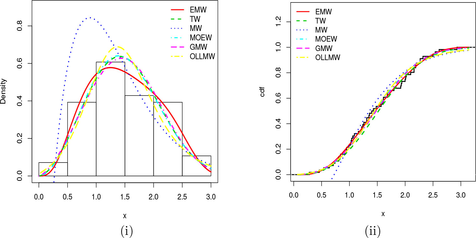
BPlots of the (i) estimated pdfs superimposed on the histogram and (ii) estimated cdfs compared to the empirical cdf for Carbon dioxide.
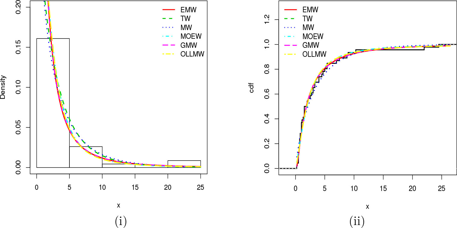
BPlots of the (i) estimated pdfs superimposed on the histogram and (ii) estimated cdfs compared to the empirical cdf for Airborne.

Plots of the (i) estimated pdfs superimposed on the histogram and (ii) estimated cdfs compared to the empirical cdf for Rainfall.
Visually, the fits of the EMW model seem better to the others. We now put an emphasis on the EMW model fitting in Figures 9, 10 and 11, showing the previous graphics without the other models, and by the consideration of the probability-probability (P-P) plots and the quantilequantile (Q-Q) plots, where nice fits of the considered distribution over the data is characterized by a nice adjustment of the scatter plot by the P-P or Q-Q lines, respectively.

Plots of the estimated pdf superimposed on the histogram, estimated cdf compared to the empirical cdf, P-P plot and Q-Q plot for the EMW model for Carbon dioxide.

Plots of the estimated pdf superimposed on the histogram, estimated cdf compared to the empirical cdf, P-P plot and Q-Q plot for the EMW model for Airborne.

Plots of the estimated pdf superimposed on the histogram, estimated cdf compared to the empirical cdf, P-P plot and Q-Q plot for the EMW model for Rainfall.
As expected, in all the situations, very adequate fits are observed for the EMW distribution.
6 Concluding remarks
Along this study, the EMW distribution is proved to be veritably versatile. Among other desirable properties, it can produce increasing, decreasing, constant, upside-down bathtub and bathtub shapes for the corresponding hazard rate function. The flexibility of the EMW model was further confirmed by applying it to fit three practical data sets, and comparing the EMW model to other well-established models by the means of several goodness-of-fit statistics. In practice, the EMW model ought to be more realistic and useful than its original counterpart and the proposed extended models should lead to further advances in biostatistics, hydrology, meteorology, survival analysis and engineering, among several other fields of research that have already benefited from the utilization of existing related models. Last but not least, the EMW distribution comes from the new and more general U family, which can be an independent source of inspiration for the statisticians in view of other purposes and applications.
Acknowledgement
The authors would like to warmly thank the reviewer for constructive comments on the paper.
REFERENCES
1 [1] AARSET, M. G.: How to identify a bathtub hazard rate, IEEE Transactions on Reliability 36(1987), 106–108.10.1109/TR.1987.5222310Search in Google Scholar
2 [2] ALZAATREH, A.—LEE, C.—FAMOYE, F.: A new method for generating families of continuous distributions,Metron 71(2013), 63–79.10.1007/s40300-013-0007-ySearch in Google Scholar
3 [3] ARYAL, G. R.—TSOKOS, C. P.: Transmuted Weibull distribution: A generalization of the Weibull probability distribution, Eur. J. Pure Appl. Math. 4(2011), 89–102.Search in Google Scholar
4 [4] ASHOUR, S.—ELTEHIWY, M.: Exponentiated power Lindley distribution, J. Adv. Res. 6(2014), 895–905.10.1016/j.jare.2014.08.005Search in Google Scholar
5 [5] ASLAM, M.—ARIF, O. H.—JUN, C. H.: An attribute control chart for a Weibull distribution under accelerated hybrid censoring, PloS ONE 12(3) (2017), e0173406.10.1371/journal.pone.0173406Search in Google Scholar
6 [6] BAIN, L. J.: Analysis for the linear failure-rate life-testing distribution, Technometrics 16(1974), 551–559.10.1080/00401706.1974.10489237Search in Google Scholar
7 [7] BIRNBAUM, Z. W.—MCCARTY, B. C.: A distribution-free upper confidence bounds for Pr(Y¦X) based on independent samples of X and Y, Ann. Math. Statist. 29(1958), 558–562.10.1214/aoms/1177706631Search in Google Scholar
8 [8] CARRASCO, J. M.—ORTEGA, E. M.—CORDEIRO, G. M.: A generalized modified Weibull distribution for lifetime modeling, Comput. Statist. Data Anal. 53(2008), 450–462.10.1016/j.csda.2008.08.023Search in Google Scholar
9 [9] CHEN, Z.: A new two-parameter lifetime distribution with bathtub shape or increasing failure rate function,Stat. Probab. Lett. 49(2000), 155–161.10.1016/S0167-7152(00)00044-4Search in Google Scholar
10 [10] CORZO, O.—BRACHO, N.: Application of Weibull distribution model to describe the vacuum pulse osmotic dehydration of sardine sheets, LWT-Food Science and Technology 41(2008), 1108–1115.10.1016/j.lwt.2007.06.018Search in Google Scholar
11 [11] GHITANY, M. E.—AL-MUTAIRI, D. K.—BALAKRISHNAN, N.—AL-ENEZI, L. J.: Power Lindley distribution and associated inference, Comput. Statist. Data Anal. 64(2013), 20–33.10.1016/j.csda.2013.02.026Search in Google Scholar
12 [12] GUPTA, R. D.—KUNDU, D.: Generalized exponential distribution, Aust. N. Z. J. Stat. 41(1999), 173–188.10.1111/1467-842X.00072Search in Google Scholar
13 [13] IBRAHIM, N. A.—KHALEEL, M. A.—MEROVCI, F.: Weibull Burr X distribution properties and application,Pakistan J. Statist. 33(2017), 315–336.Search in Google Scholar
14 [14] KOTZ, S.—LUMELSKII, Y.—PENSKY, M.: The Stress-Strength Model and its Generalizations, World Scientific Press, Singapore, 2003.10.1142/5015Search in Google Scholar
15 [15] LEHMANN, E. L.: Ordered families of distributions, Ann. Math. Stat. 26(1955), 399–419.10.1007/978-1-4614-1412-4_60Search in Google Scholar
16 [16] LINDLEY, D. V.: Fiducial distributions and Bayes’ theorem, J. Roy. Statist. Soc. Ser. A 20(1958), 102–107.10.1111/j.2517-6161.1958.tb00278.xSearch in Google Scholar
17 [17] MUDHOLKAR, G. S.—SRIVASTAVA, D. K.: Exponentiated Weibull family for analyzing bathtub failure-rate data, IEEE Transactions on Reliability 42(1993), 299–302.10.1109/24.229504Search in Google Scholar
18 [18] NIKULIN, M.—HAGHIGHI, F.: A chi-squared test for the generalized power Weibull family for the head-and-neck cancer censored data, J. Math. Sci. 133(2006), 1333–1341.10.1007/s10958-006-0043-8Search in Google Scholar
19 [19] PENG, X.—YAN, Z.: Estimation and application for a new extended Weibull distribution, Reliab. Eng. Syst. Saf. 121(2014), 34–42.10.1016/j.ress.2013.07.007Search in Google Scholar
20 [20] POGANY, T. K.—SABOOR, A.—PROVOST, S.: The Marshall-Olkin exponential Weibull distribution, Hacet. J. Math. Stat. 44(2015), 1579–1594.10.15672/HJMS.2015478614Search in Google Scholar
21 [21] R DEVELOPMENT CORE TEAM: R: A language and environment for statistical computing, R Foundation for Statistical Computing, Vienna, Austria, 2005.Search in Google Scholar
22 [22] SABOOR, A.—ALIZADEH, M.—KHAN, M. N.—GOSH, I.—CORDEIRO, G. M.: Odd Log-Logistic modified Weibull distribution, Mediterr. J. Math. 14(2017), 1–19.10.1007/s00009-017-0880-3Search in Google Scholar
23 [23] SARHAN, A. M.—KUNDU, D.: Generalized linear failure rate distribution, Comm. Statist. Theory Methods 38(2009), 642–660.10.1080/03610920802272414Search in Google Scholar
24 [24] SARHAN, A. M.—ZAINDIN, M.: Modified Weibull distribution, Appl. Sci. 11(2009), 123–136.Search in Google Scholar
25 [25] VON ALVEN, W. H.: Reliability Engineering by ARINC, Prentice-hall, New Jersey, 1964.Search in Google Scholar
26 [26] WANG, Y.—CHAN, Y.—GUI, Z.—WEBB, D.—LI, L.: Application of Weibull distribution analysis to the dielectric failure of multilayer ceramic capacitors, Mater. Sci. Eng. B 47(1997), 197–203.10.1016/S0921-5107(97)00041-XSearch in Google Scholar
27 [27] XIE, M.—LAI, C. D.: Reliability analysis using an additive Weibull model with bathtub-shaped failure rate function, Reliab. Eng. Syst. Saf. 52(1995), 87–93.10.1016/0951-8320(95)00149-2Search in Google Scholar
© 2022 Mathematical Institute Slovak Academy of Sciences
This work is licensed under the Creative Commons Attribution 4.0 International License.
Articles in the same Issue
- Mathematica Slovaca
- Expanding Lattice Ordered Abelian Groups to Riesz Spaces
- Ordinary Generating Functions of Binary Products of Third-Order Recurrence Relations and 2-Orthogonal Polynomials
- Quartic Polynomials with a Given Discriminant
- Joint Approximation by Dirichlet L-Functions
- Generalizations of Hardy Type Inequalities by Taylor’s Formula
- Certain Estimates of Normalized Analytic Functions
- Oscillation of Second Order Delay Differential Equations with Nonlinear Nonpositive Neutral Term
- Existence and Multiplicity of Radially Symmetric k-Admissible Solutions for Dirichlet Problem of k-Hessian Equations
- Existence and Asymptotic Periodicity of Solutions for Neutral Integro-Differential Evolution Equations with Infinite Delay
- Approximation Properties of λ-Bernstein-Kantorovich-Stancu Operators
- A Korovkin Type Approximation Theorem For Balázs Type Bleimann, Butzer and Hahn Operators via Power Series Statistical Convergence
- Hyperbolic Geometry For Non-Differential Topologists
- Set Star-Menger and Set Strongly Star-Menger Spaces
- Some Characterizations of Mixed Renewal Processes
- The U Family of Distributions: Properties and Applications
- A New Method for Generalizing Burr and Related Distributions
- On Mahler's Classification of Formal Power Series Over a Finite Field