Investigating the ecological fallacy through sampling distributions constructed from finite populations
-
 and
and

Abstract
Correlation coefficients and linear regression values computed from group averages can differ from correlation coefficients and linear regression values computed using individual scores. This observation known as the ecological fallacy often assumes that all the individual scores are available from a population. In many situations, one must use a sample from the larger population. In such cases, the computed correlation coefficient and linear regression values will depend on the sample that is chosen and the underlying sampling distribution. The sampling distribution of correlation coefficients and linear regression values for group averages will be identical to the sampling distribution for individuals for normally distributed variables for random samples drawn from infinitely large continuous distributions. However, data that is acquired in practice is often acquired when sampling without replacement from a finite population. Our objective is to demonstrate through Monte Carlo simulations that the sampling distributions for correlation and linear regression will also be similar for individuals and group averages when sampling without replacement from normally distributed variables. These simulations suggest that when a random sample from a population is selected, the correlation coefficients and linear regression values computed from individual scores will not be more accurate in estimating the entire population values compared to samples when group averages are used as long as the sample size is the same.
1 Introduction
Linear regression coefficients, the Pearson R correlation, and the coefficient of determination
A mathematical analysis of the ecological fallacy [13] assumes a fixed set of scores that generate different linear regression coefficients or correlation values depending on whether the individual scores are used or whether they are averaged first. However, the scores may not necessarily represent an entire population. In many situations, the individual scores are themselves a sample. In such situations, the computed values of the correlation and regression coefficients of the sample of individuals are estimates of the population coefficients. The accuracy of the estimates depends on the underlying sampling distribution. Analytical sampling distributions have been derived for the Pearson R coefficient [2], coefficient of determination
Less is known when sampling without replacement from finite populations which is the way data is acquired in many practical situations.
This article employs Monte Carlo simulations to suggest that the R,
The paper is organized as follows. Section 2 introduces the notation used in the paper and describes the analytical sampling distributions of R,
2 Nomenclature and analytical sampling distributions
Nomenclature used in manuscript.
| N | Size of the population |
| n | Sample size |
|
|
Sample percent of population |
| m | Group size |
|
|
Total number of scores used in sample = nm |
| k | Number of independent variables |
| R | Sample correlation coefficient |
|
|
Sample coefficient of determination |
| b | Sample regression slope |
|
|
Expectation of analytical sampling distributions |
|
|
Variance of analytical sampling distributions |
|
|
Expectation of simulation sampling distributions |
|
|
Variance of simulation sampling distributions |
| ρ | Correlation of continuous distribution |
|
|
Coefficient of determination of continuous distribution |
|
|
Means from bivariate distribution |
|
|
Standard deviation from bivariate distribution |
|
|
Bivariate distribution |
| B | Beta function |
|
|
Generalized hypergeometric function |
|
|
Percent relative difference in Pearson R variance,
|
|
|
Percent relative difference in
|
|
|
Percent relative difference in slope b variance,
|
|
|
Percent relative difference in Fisher variance,
|
We refer the reader to Table 1 which lists the symbols and their descriptions that are used in the manuscript.
Muirhead [12] notes that samples
(2.1)
with ρ the continuous population correlation, means
where Γ is the gamma function,
whose distribution approaches a normal distribution
as
Gatignon [5] notes that averages
follow the distribution
where
The expectation
The
In regards to the simple regression slope b, samples of size n drawn from a bivariate distribution generate the distribution
If group averages are used, both
If we let
the distribution (2.9) becomes a t-distribution with ν degrees of freedom which can be approximated by a normal distribution for large n.
When more than one independent variable is used, the distribution of samples of size n drawn from a multivariate normal distribution generate the coefficient of determination
where B is the beta function,
3 Method: Monte Carlo simulations
3.1 Comparing simple linear regression distributions
We begin our investigation by generating a population of scores
where
Subsequently, we randomly select n groups of scores of size m. Since the sampling is done without replacement, we require that
Figure 1 shows the results of the Monte Carlo simulations of the Pearson R correlation coefficient and linear regression slope using a population of
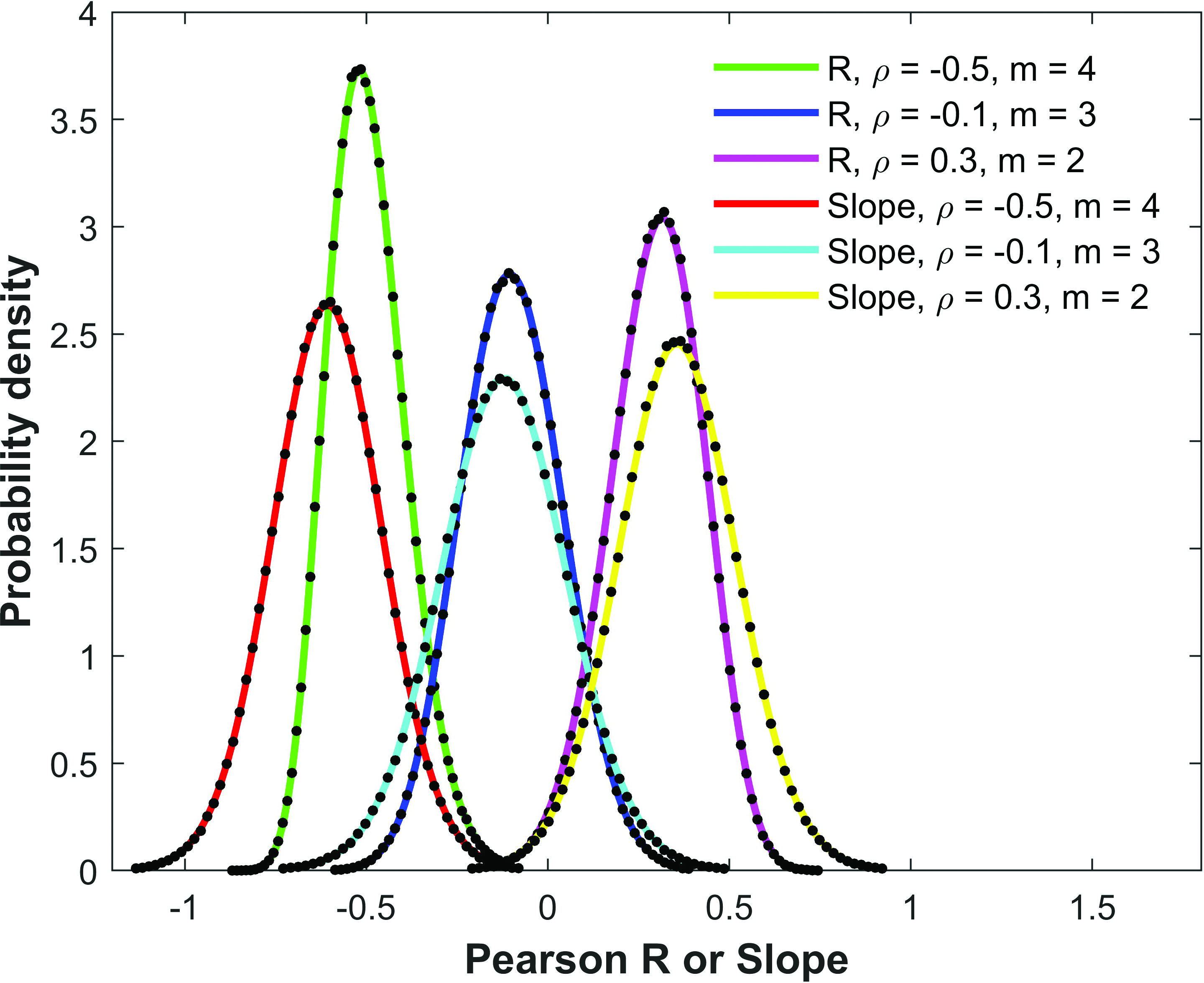
Comparison of the Monte Carlo simulation distributions (black dots) of Pearson R and linear regression slope using

Comparison of Monte Carlo simulation distributions (black dots and lines) of Pearson R and linear regression slope using
Figure 2 shows the results of the Monte Carlo simulations of the Pearson R correlation coefficient and linear regression slope conducted under the same conditions as Figure 1 except that a population of
Differences when comparing the analytical and simulation distribution expectation and variance in Figures 1 and 2.
| Figure 1: Sample size
|
||||
| ρ |
|
Percent relative difference in
|
|
Percent relative difference in
|
| -0.5 |
|
-0.26 |
|
-0.56 |
| -0.1 |
|
-0.01 |
|
-0.04 |
| 0.3 |
|
-1.45 |
|
-1.11 |
| Figure 2: Sample size
|
||||
| ρ |
|
Percent relative difference in
|
|
Percent relative difference in
|
| -0.5 |
|
-24.4 |
|
-24.6 |
| -0.1 |
|
-23.4 |
|
-24.0 |
| 0.3 |
|
-22.3 |
|
-23.2 |
Table 2 shows the differences in the simulated and analytical expected value of R,
for
Figures 1 and 2. Table 2 shows that the differences in the expectation are small for both figures. However the percent relative differences in the variance of R and b are large in Figure 2 (ranging between
3.2 Comparing multiple regression distributions
For multiple regression simulations, we use the Cholesky decomposition [11] to correlate the variables. If
Figure 3 shows the results of the Monte Carlo simulation that generates the distribution of the coefficient of determination

Comparison of Monte Carlo simulations (black dots) and analytical distributions of Pearson

Comparison of Monte Carlo simulations (black lines and dots) and analytical distributions of Pearson
Figure 4 shows the results of the Monte Carlo simulations of the coefficient of determination
Table 3 shows the differences in the simulated and analytical expected value of
for
Figures 3 and 4. Table 3 shows that the differences in the expectation are small for both figures. However the percent relative difference in the variance of
| Figure 3: Sample size
|
||||
|
|
|
Percent relative differences in
|
|
Percent relative differences in
|
| 0.26 |
|
|
|
|
| 0.73 |
|
|
|
|
| Figure 4: Sample size
|
||||
|
|
|
Percent relative differences in
|
|
Percent relative differences in
|
| 0.25 |
|
-23.0 |
|
-24.3 |
| 0.71 |
|
-24.7 |
|
-23.5 |
These first examples suggest that when sampling without replacement from normal distributions, the expectation differences between the analytical and simulated distributions are small regardless of the group size m. Differences arise between the variance of the analytical and simulated distributions when the sample size n is a significant percent of the population size N regardless of the group size m. In the next section, we explore parameter space
further to determine if the differences in the analytical and simulated expectations in R,
4 Results: Exploring parameter space
Our objective in Section 4 is to continue to explore the parameter space of ρ, m, n, and N further to determine if and where differences exist between the analytical distributions and the sampling distributions created without replacement. The parallel Fortran code is available at: https://github.com/davytorres/MonteCarloEcological.git.
In our preliminary analysis in Section 3, only one population was chosen for the simulations. We increase the number of populations to 112 (chosen because it is divisible by 8 and 14 which are the number of processors available on our computers for parallel runs) to determine if the population selection affects the observed trends. In all the simulations in Section 4, a million randomly chosen samples are used to create each distribution. The most important parameter we identified in Section 3 was the sample percent of the total population
4.1 Simple regression – Pearson R
Figure 5 plots the difference
Figure 5 shows that the difference in

Plot of difference

Plot of
We also note that the range of the error bars in Figure 5 increases as the sample percent of the population decreases. Define the range
If the
Figure 7 plots the difference

Plot of difference

Plot of difference
Figure 9 plots the percent relative difference
The average percent relative differences can be closely approximated by the linear plot
which is not a function of the group size m . The size of the error bars increases as the sample percent of the population decreases which was also observed in the Pearson R expectation plot (Figure 5).
It is well known if all samples are considered, the variance of the sampling distribution
When computing the variance when sampling without replacement
The percent relative difference between the two variances is
which is similar to the approximation (4.2)
Figure 10 plots the error (from Figure 9) when approximating the plot of
Simulations (not shown) identical to Figure 10 were conducted except that a small population
To further test the validity of (4.2), we fit a linear regression line through the plot of

Plot of percent relative difference

Plot of error
The ecological fallacy can be viewed from the following perspective for normally distributed variables and random sampling.
Note that the total number of scores
4.2 Testing Fisher’s approximation
Since the distribution of R is not symmetric about the mean, we investigated properties of the Fisher transformed (2.3) values of R as the transformed distribution is approximately normal and is useful in building confidence intervals. Recall from (2.4) that as
and variance
Figures 11–13 use the same data and parameters from the simulations described in Figures 5–10.
Figure 11 plots the average difference
variables created by Monte Carlo simulations with
Figure 12 plots the average percent relative difference in the variance
where
We have compared the expectation and variances of the Pearson R distribution. To compare the simulated and analytical distribution functions, we use the Fisher transformed variables. Figure 13 plots the average error
where
and

Plot of difference

Plot of percent relative difference

Plot of error
4.3 Simple regression – Slope
Figures 14–18 use the same data from the simulations described in
Figures 5–10.
Figure 14 plots the difference

Plot of difference

Plot of difference

Plot of difference

Plot of percent relative difference

Plot of error
Similar to Figure 5, the range of the error bars in Figure 14 increases as the sample percent of the population decreases. Define the range
If the
Figure 15 plots the difference
Figure 17 plots the percent relative difference
using a population size
where
Simulations (not shown) identical to Figure 18 were conducted except that a small population
To test the validity of (4.5), we fit a linear regression line through the plot of
4.4 Groups of mixed size
In Figures 19–22, we study the behavior of groups of mixed size.
In all the figures, the population size is

Plot of difference

Plot of difference

Plot of percent relative difference

Plot of percent relative difference
There are equal amounts of each group size in each sample.
The plot symbol shows the average difference and the error bars show the maximum and minimum errors using 112 different populations. The differences in the expectation values remain small. However, the size of the error bars increases as the sample percent of the population
Figure 21 and Figure 22 plot
4.5 Non-normal populations
In this subsection, we consider random samples drawn from non-normal distributions.
In all Figures 23–35, the population size is
and a bimodal distribution
respectively. The plot symbol shows the average difference and the error bars show the maximum and minimum differences using 112 different populations. The average differences are small but their absolute values increase as the sample percent of the population

Plot of difference

Plot of difference

Plot of difference

Plot of percent relative difference

Plot of percent relative difference

Plot of percent relative difference

Plot of difference

Plot of difference

Plot of difference

Plot of percent relative difference

Plot of percent relative difference

Plot of percent relative difference

Plot of difference
Figure 26, Figure 27, and Figure 28 plot
Figure 29, Figure 30, and Figure 31 plot the difference
Figure 32, Figure 33, and Figure 34 plot
Figure 35 plots the area difference
4.6 Multiple regression results
We move now to multiple regression simulations.
Figure 36 plots the difference

Plot of difference

Plot of percent relative difference

Plot of difference

Plot of percent relative difference
Figure 37 plots the percent relative difference
Figure 38 plots the difference
Figure 39 plots the percent relative difference
5 Discussion and conclusion
In this article, we perform Monte Carlo simulations to select samples without replacement from finite populations to generate distributions of Pearson R, slope b, and the coefficient of determination
However the variances of the R, b, and
The distribution of the Fisher transformed value of R denoted by
We also observed that for non-normal distributions, the percent relative differences in the correlation variances
Our observations afford another interpretation of the ecological fallacy and suggest that for random samples drawn without replacement from normally distributed finite populations, the correlation coefficients and linear regression slopes will be selected from approximately the same sampling distribution regardless of the group size m as long as the sample size n is the same.
Funding source: National Institute of General Medical Sciences
Award Identifier / Grant number: P20GM103451
Funding statement: This research is supported by an Institutional Development Award (IDeA) from the National Institute of General Medical Sciences of the National Institutes of Health under grant number P20GM103451. The content is solely the responsibility of the author and does not necessarily represent the official views of the National Institutes of Health. We also received support from the Sustainable Research Pathways program and the Sustainable Horizons Institute.
A Appendix: Fortran code
The parallel Fortran code we use to run the Monte Carlo simulations evenly divides the 112 populations among the processors. Each processor then develops the Pearson R and slope distributions using its share of the populations for different values of group size m and different sample percents of the population
Each processor finds the maximum, minimum, and average difference of the expectation and variance of each distribution from the analytical value for its share of the populations. Then the maximum, minimum, and average difference of the expectation and variance are shared among all the processors, to find the maximum, minimum, and average difference for all populations which is stored on the first processor.
We have developed two versions of the code: an MPI version and a Coarray Fortran version. MPI uses the MPI_REDUCE calls for communication and the Coarray Fortran uses the co_sum, co_max, and co_min calls for communication.
References
[1] N. Cleave, P. J. Brown and C. D. Payne, Evaluation of methods for ecological inference, J. Roy. Statist. Soc. Ser. A 158 (1995), 55–72. 10.2307/2983403Search in Google Scholar
[2] R. A. Fisher, Frequency distribution of the values of the correlation coefficient in samples from an indefinitely large population, Biometrika 10 (1915), 507–521. 10.1093/biomet/10.4.507Search in Google Scholar
[3] R. A. Fisher, On the probable error of a coefficient of correlation deduced from a small sample, Metron 1 (1921), 3–32. Search in Google Scholar
[4] R. A. Fisher, The general sampling distribution of the multiple correlation coefficient, Proc. Roy. Soc. Lond. Ser. A 121 (1928), 654–673. 10.1098/rspa.1928.0224Search in Google Scholar
[5] H. Gatignon, Statistical Analysis of Management Data, 2nd ed., Springer, New York, 2010. 10.1007/978-1-4419-1270-1Search in Google Scholar
[6] A. T. Geronimus and J. Bound, Use of census-based aggregate variables to proxy for socioeconomic group: Evidence from national samples, Am. J. Epidemiol. 148 (1988), 475–486. 10.1093/oxfordjournals.aje.a009673Search in Google Scholar PubMed
[7] L. Goodman, Ecological regressions and behavior of individuals, Amer. Sociological Rev. 18 (1953), 663–664. 10.2307/2088121Search in Google Scholar
[8] L. Irwin and A. J. Lichtman, Across the great divide: Inferring individual level behavior from aggregate data, Political Methodology 3 (1976), 411–439. Search in Google Scholar
[9] G. King, A Solution to the Ecological Inference Problem: Reconstructing Individual Behavior from Aggregate Data, Princeton University, New Jersey, 1997. 10.3886/ICPSR01132Search in Google Scholar
[10] A. J. Lichtman, Correlation, regression, and the ecological fallacy: A critique, J. Interdiscip. Hist. 4 (1974), 417–433. 10.2307/202485Search in Google Scholar
[11] S. Mahadevan, Monte Carlo simulation, Reliability-Based Mechanical Design, Marcel Dekker, New York (1997), 123–146. Search in Google Scholar
[12] R. J. Muirhead, Aspects of Multivariate Statistical Theory, John Wiley & Sons, New Jersey, 2005. Search in Google Scholar
[13] S. Piantadosi, D. P. Byar and S. B. Green, The ecological fallacy, Am. J. Epidemiol. 127 (1988), 893–904. 10.1093/oxfordjournals.aje.a114892Search in Google Scholar PubMed
[14] W. S. Robinson, Ecological correlations and the behavior of individuals, Amer. Sociological Rev. 15 (1950), 351–357. 10.2307/2087176Search in Google Scholar
[15] V. Romanovskij, On the distribution of the regression coefficient in samples from normal population, Bull. Acad. Sci. URSS 20 (1926), no. 6, 643–648. Search in Google Scholar
[16] Y. T. Shih, C. Bradley and K. R. Yabroff, Ecological and individualistic fallacies in health disparities research, J. National Cancer Inst. 115 (2023), 488–491. 10.1093/jnci/djad047Search in Google Scholar PubMed PubMed Central
[17] D. J. Torres, Describing the Pearson R distribution of aggregate data, Monte Carlo Methods Appl. 1 (2020), 17–32. 10.1515/mcma-2020-2054Search in Google Scholar PubMed PubMed Central
[18] S. M. Woodward, D. Mork, X. Wu, Z. Hou, D. Braun and F. Dominici, Combining aggregate and individual-level data to estimate individual-level associations between air pollution and COVID-19 mortality in the United States, PLOS Global Public Health 3 (2023), Article ID e0002178. 10.1371/journal.pgph.0002178Search in Google Scholar PubMed PubMed Central
© 2024 Walter de Gruyter GmbH, Berlin/Boston
This work is licensed under the Creative Commons Attribution 4.0 International License.
Articles in the same Issue
- Frontmatter
- Investigating the ecological fallacy through sampling distributions constructed from finite populations
- Bernoulli factory: The 2𝚙-coin problem
- Randomized vector algorithm with iterative refinement for solving boundary integral equations
- Application of semiclassical approximation to stochastic differential equations
- Trapezoidal and Simpson’s methods with a random design
- Periodic INAR(1) model with Bell innovations distribution
- Effect of biaxial strain on the binding energies of adsorbed In and Al atoms on (001) surfaces of InAs and AlAs
- Estimating pharmacokinetic parameters from Dynamic Contrast-Enhanced T 1-weighted MRI using a three level hierarchical Bayesian model
- Bayesian analysis of the COVID-19 pandemic using a Poisson process with change-points