Home advantage for tournament victory: empirical evidence from FIFA World Cups and continental championships
-
Adriaan Kalwij


Abstract
This study provides empirical support for a meaningful variation in home advantage (HA) for winning a cup tournament (tournament victory) by home team (HT)’s strength, arguably through compound probability. The data is on football matches between national teams at FIFA World Cups and continental championships, and on teams’ Elo rating which measures their strength. The empirical findings show that for an average cup tournament hosted by a single country, the estimated HA for tournament victory is 22 percentage points (pp) for a HT with an average Elo rating. This HA decreases to 9 pp for a HT with a one standard deviation below-average Elo rating and increases to 42 pp for a HT with a one standard deviation above-average Elo rating. Hence, the stronger the HT, the larger is its expected HA for tournament victory. The tournament outcome of an away team (AT) can, therefore, also be affected by which country hosts the cup tournament. That is, a larger HA for tournament victory for the HT, or HTs in the case of multiple host countries, is also a larger disadvantage for the ATs.
1 Introduction
In a football league, a team usually plays one match at home and one match away against each competing team during the season, which can nullify home advantage (HA) for each team’s standing at the end of the season (Pollard 2006). Likewise for HA for qualifying to compete at final FIFA World Cups or championships for national teams organized by the six FIFA-affiliated continental confederations – henceforth referred to as cup tournaments – because a qualifying stage most often consists of two-legged ties with home and away matches. Cup (final) tournaments most often have a different setup with respect to playing at home or away. They are most often hosted by a single country and the host country’s team has HA in all their matches while the other national teams do not have HA in any of their matches. Hence, unlike for, e.g., a football league, HA can affect a national team’s final standing at the end of such a cup tournament. A particular concern this study addresses is that HA for the final standing can be mitigated or reinforced by the home team’s strength through compound probability.
Therefore, this study examines empirically HA in cup (final) tournaments and, more specifically, the extent to which HA for winning a cup tournament varies by home team’s strength. The relevance of obtaining empirical insight in such variation for sports tournaments with a single host country (or a few host countries), and where HA exists, is that it can cause a tournament’s host country to affect – through a combination of the home team’s strength and compound probability – the tournament outcomes of all teams.
The international governing body of association football FIFA (Fédération Internationale de Football Association; www.fifa.com) and its affiliated six continental confederations run cup tournaments for national football teams at regular intervals. Any country can bid to host a cup tournament. An argument for placing a bid is that the country’s gains from, e.g., increased tourism revenue or increased interest in the game of football, exceed its costs such as infrastructural investments (Coates and Humphreys 2008; Falter et al. 2008; Mitchell and Stewart 2015; Szymanski and Drut 2020). Hosting a cup tournament can also contribute to the success of the national team, like for hosting the Olympic Games (Rewilak 2021), which can have fundamental societal impact through building national identity (Depetris-Chauvin et al. 2020). The organizing body uses a ballot system to decide which bid to accept, thereby determining the host country, or host countries, for the next cup tournament. The host country’s team, i.e., the home team (HT), can enjoy home advantage (HA) for winning matches at the tournament – henceforth referred to as HA for winning a match. That is, such HA refers to the phenomenon that the HT is more likely to win a match than an away team (AT), conditional on their strength, arguably because of, e.g., crowd effects on players and referees, visitors’ travel fatigue, venue familiarity, or playing tactics (Bryson et al. 2021; Gómez-Ruano et al. 2022; Pollard 2008; Pollard and Armatas 2017; Staufenbiel et al. 2015).
The organizing body of a cup tournament is most likely aware of HA affecting tournament outcomes because HA for winning matches is a well-documented phenomenon (Gómez-Ruano et al. 2022; Pollard 2006; Schwartz and Barsky 1977). For instance, for FIFA World Cup qualifying matches national teams’ percentage of points won at home varied from, on average, 56 % for European teams to 70 % for African teams (Brown et al. 2002; Pollard and Armatas 2017). Also, for the 2002 World Cup Torgler (2004) estimated that playing at home increased the probability of winning a match by 45 percentage points (pp).
The organizing body can be less aware of the effect a tournament’s host country has, through HT’s strength, on HA for winning a tournament – henceforth referred to as HA for tournament victory – because there is only suggestive empirical evidence on this. Nevertheless, the evidence suggests that such HA can be substantial: six of the 22 World Cup tournaments, played since 1930, were won by home teams (Dowie 1982; www.fifa.com). These latter winning HTs were also among the best teams in the world, which makes it difficult to draw conclusions. Also, Monks and Husch (2009) show that there was a significant HA effect on the final standing at the 1982–2006 World Cups of teams playing near to home, i.e., if the team’s country was on the same continent as the tournament’s host country.
This study contributes to the empirical literature by quantifying the extent to which HT’s strength affects its ex ante HA for tournament victory. A statistical argument for such an effect is compound probability (Appendix A.1 provides a simple exposition of this mechanism). The argument is most apparent for a tournament with a knockout stage: a (relatively) strong HT has a higher probability of surviving each round of the tournament, hence of reaching the final match, than a weak HT and has therefore in expectation a higher HA for tournament victory. Another argument is that HT’s strength can affect HA in performance (Pollard 2008), hence can affect HA for tournament victory. For instance, because a HT’s strength can determine the size of the home crowd which, arguably, affects the HA (Bryson et al. 2021). These two arguments show that the tournament’s host country can affect not only the tournament outcome of the HT but also the tournament outcomes of the ATs; a HA for the HT equals the sum of the away disadvantages for the ATs. Hence, for an AT it can matter for its tournament outcome in which country the tournament is played. Furthermore, the two arguments also apply to variation by HT’s strength in HA for other tournament outcomes such as reaching the quarterfinals. Finally, factors such as choking under pressure or seeding can also cause variation in HA for tournament victory by HT’s strength (Baumeister and Steinhilber 1984; Jordet et al. 2012; Monks and Husch 2009). Hence, it is an empirical matter if there is on average a meaningful variation in HA for tournament victory by HT’s strength at cup tournaments.
This study employs data of football matches from cup tournaments for men’s national teams to examine HA for tournament victory and, more importantly, the extent to which this HA varies by HT’s strength. The empirical analysis is based on the outcomes of football matches played between 1916 and 2024 at 177 cup tournaments, and on teams’ Elo rating which measures their (relative) strength, i.e., their ability to perform (Section 2.1). Logistic regression models are used for estimating the effects of playing at home and teams’ Elo rating on the probability of winning a match and on the probability of tournament victory (Section 2.2). Based on the estimation results, HA for winning a match and HA for tournament victory are quantified by HT’s Elo rating (Section 3). The main empirical findings support that there is through compound probability a meaningful variation in HA for tournament victory by HT’s strength, measured by its Elo rating. Section 4 discusses the main empirical findings.
2 Materials and methods
2.1 The data
2.1.1 Data on football matches
The results of 4,091 matches played between 1916 and 2024 at the final tournaments of all editions of the FIFA World Cup and championships for national teams organized by the six continental confederations are available from various public online sources (Appendix A.2). The selected six championships are the AFC Asian Cup, Africa Cup of Nations, CONCACAF Gold Cup, CONMEBOL Copa América, OFC Nations Cup, and UEFA European Football Championship. The data also contains information on the host countries, stages, and rounds of the tournaments. A group stage usually has a round-robin setup. Most tournaments have a knockout stage that consists of at least one elimination round (a round-of-16, quarterfinals, semi-finals, third place playoff, or final match).
In weighing the result of a match, we considered which of the two competing national teams won a match. This result is referred to as the outcome of a match. Matches played in the group stage generally have the possibility of ending in a draw, while matches played in the knockout stage do not have this possibility. If a knockout match ended in a draw after playing the regular 90 min and still having no decision after possible extra time, a penalty shootout determined the winner since about the mid-1970s. Before then such a draw was dealt with in various ways. For instance, with a rematch for the final match at the 1975 Copa America or a coin toss for the semi-final between Italy and the Soviet Union at the 1968 UEFA European Football Championship.
Further, the country where the match was played determines if a team is a HT or an AT. Of the 177 cup tournaments, 156 were hosted by a single country and 21 were hosted by multiple host countries. Of these 21 tournaments, six consisted of two-legged ties with home and away matches such that the countries of all participating teams were host countries.
No matches are excluded and the estimation sample, therefore, consists of the outcomes of 4,091 matches played between 1916 and 2024 by 158 national teams at 177 cup tournaments. Table 1 provides information on the numbers of tournaments, of teams and of matches by cup tournament.
Numbers of tournaments, teams and matches, and the average Elo rating.
| Cup tournament | Cup tournaments | Matches | Teams | |||||
|---|---|---|---|---|---|---|---|---|
| All | A single host country | Multiple host countries | All | Can draw | Cannot draw | All | Elo rating | |
| (Period) | N1 | N1 | N1 | N2 | N2 | N2 | N3 | Mean (SD) |
| AFC Asian Cup | 18 | 17 | 1 | 422 | 317 | 105 | 36 | 1,512 |
| (1956–2023/24) | (161) | |||||||
| Africa Cup of Nations | 34 | 32 | 2 | 793 | 579 | 214 | 44 | 1,564 |
| (1957–2023/24) | (118) | |||||||
| CONCACAF Gold Cup | 27 | 21 | 6 | 514 | 408 | 106 | 28 | 1,576 |
| (1963–2023) | (171) | |||||||
| CONMEBOL Copa | 48 | 45 | 3 | 869 | 761 | 108 | 20 | 1,753 |
| América (1916–2024) | (203) | |||||||
| OFC Nations Cup | 11 | 7 | 4 | 141 | 114 | 27 | 10 | 1,293 |
| (1973–2024) | (247) | |||||||
| UEFA European football championship | 17 | 13 | 4 | 388 | 277 | 111 | 36 | 1,877 |
| (1960–2024) | (112) | |||||||
| FIFA World Cup | 22 | 21 | 1 | 964 | 752 | 212 | 80 | 1,827 |
| (1930–2022) | (139) | |||||||
| Total | 177 | 156 | 21 | 4,091 | 3,208 | 883 | 158 | 1,682 |
| (154) | ||||||||
-
Notes. Sample: see Section 2. N1, number of cup tournaments; N2, number of matches; N3, number of teams; and SD, standard deviation. The SDs are computed for Elo ratings in difference from their averages by cup tournament and edition. The current names of cup tournaments are used. The FIFA-affiliated continental confederations are listed in Appendix A.2.
2.1.2 Data on teams’ Elo ratings
The estimation sample described in Section 2.1.1 is supplemented with the teams’ Elo ratings as measured at the end of the calendar year preceding the year of the tournament. Table 1 provides information on the average Elo rating by cup tournament. National football teams’ Elo ratings are publicly available (Appendix A.2). The Elo ratings are measures of relative abilities to perform (Elo 1978; Gásquez and Royuela 2016). That is, a team’s Elo rating is based on performances before the tournament and indicates a team’s strength relative to other national teams’ strength at a given point in time. Elo ratings are available for the whole observation period. Elo ratings, or related ratings (Baker and McHale 2018), have been used to measure the strength of national football teams in empirical works (Krumer and Moreno-Ternero 2023; Lapré and Palazzolo 2022, 2023) and in simulation studies (Chater et al. 2021; Csató 2023a,b; Stronka 2024).
Teams’ Elo ratings are expected to be closely related to FIFA’s ranking of nation teams, as both measures are based on the past performances of teams. The FIFA rankings are available from 1992 onward (Appendix A.2). The rank correlation between the annual ranking based on teams’ Elo rating and the FIFA ranking is 0.90 for the period 1992–2023. Since 2018 the FIFA’s rating of national teams is also based on an Elo system and the correlation coefficient of FIFA’s ratings with our Elo ratings is 0.96. See Szczecinski and Roatis (2022) for a discussion on FIFA’s rating systems.
2.2 Empirical framework
2.2.1 A statistical model for estimating HA for winning a match
Tullock’s (1980) rent-seeking contest model or Lazear and Rosen’s (1981) rank-order tournament model provides a game-theoretical basis for the logit models used for estimating the effects of playing at home and teams’ Elo rating on the probability of winning a match (see also Csató 2024; Jia et al. 2013; Kooreman and Schoonbeek 1997; Nalebuff and Stiglitz 1983; Nitzan 1994).
The setup of the empirical model is as follows. A match is played between national teams i and j with Elo ratings Elo i and Elo j , respectively. Hence, the difference in teams’ strength is measured by the difference in their Elo rating. The binary variable HT i equals 1 if team i played at home and equals 0 otherwise. If there is a match with a HT, team i is the HT and team j is the AT. Hence, in this setup, HT j always equals 0. What matters for the outcome of a match is the difference in teams’ performance. The expected difference is assumed a linear function of the difference in the teams’ Elo rating (ΔElo) and the HT effect on performance. The latter effect is allowed to vary with ΔElo. The binary variable D denotes if a match can end in a draw (D = 1; D = 0 for knockout matches). Given this setup, the probability that team i wins the match against team j is
where ΔEloi,j = Elo
i
− Elo
j
and with parameters
The model of Equation (1) is a logit model and estimated with maximum likelihood (Wooldridge 2010). The standard errors are clustered at the tournament level. Further, the effect of HT is identified by having outcomes of matches between a HT and an AT, and between two ATs.
Next, a HT’s HA for winning a match is quantified for a knockout match (D = 0) as the difference between the probability that the team will win if the match is played at home (HT = 1) and the probability that the team will win if the match were to be played away against an AT (HT = 0):
HA for winning a match is computed by replacing the parameter vector β in Equation (2) with its maximum likelihood estimate based on the logit model of Equation (1). HA is quantified for values of ΔElo in the range −400 to 400; approximately from the 5th percentile up to the 95th percentile of the empirical distribution of ΔElo.
2.2.2 A statistical model for estimating HA for tournament victory
Cup tournaments differ in their setups, e.g., different match schedules and knockout stages, and the distribution of tournament victory can be positively skewed because of compound probability. These features necessitate approximating the probability distribution of tournament victory for the empirical analysis. Ex ante, i.e., before the match schedule is known, the probability that team i wins cup tournament c depends, among other things, on the strength of the participating teams which is approximated with their average Elo rating
where
We assume that HA for tournament victory decreases with an increase in the number of host countries NH. The latter relationship is modelled as HT/NH and is tested against a specification that allows for different effects for tournaments with single and multiple host countries. It is expected that the higher a team’s Elo rating relative to the average Elo rating of the tournament’s participants, the higher is its probability of tournament victory
We quantify HA for tournament victory as the difference between the probability of tournament victory when the tournament is played at home (HT = 1) and the probability of tournament victory when the tournament is played away (HT = 0). Also, we consider a tournament with a single host country (NH = 1). Therefore, and using Equation (3), HA for tournament victory is
HA for tournament victory is quantified for the range of
Finally, the relative difference between HA for tournament victory (Equation (4)) and HA for winning a match (Equation (2)), i.e.,
3 Empirical results
Following the recommendations of Benjamin et al. (2018) and Benjamin and Berger (2019), a statistical finding that is significant at the 0.5 % level is plausibly replicable and treated as empirical evidence against the null hypothesis. Significance at the 5 % level, and not at the 0.5 % level, is considered suggestive evidence. Also, when interpreting empirical findings, the 154 points standard deviation (SD) of the Elo rating shown in Table 1 (bottom row) is rounded to 150 points because predictions based on Equations (2) and (4) were made with steps of 10 Elo points.
3.1 Descriptive statistics
When both teams played away matches, teams played a draw in 25 % of their matches (Table 2; top rows, first column), hence there was in 37.5 % of matches a win for one of the teams ((100 %–25 %)/2, or Table 2; top rows, first column with (36.9 + 38.1)/2 = 37.5). Team 1 won 60.3 % of their matches that could end in a draw when played at home (Table 2; middle rows, first column). Hence, for matches that could end in a draw, HA for winning a match is 60.3–37.5, which equals 22.8 pp (Table 2; bottom rows, first column). Likewise, for knockout matches (no possibility of a draw), the proportion won is of course equal to 50 % (Table 2; top rows, second column with (48.3 + 51.7)/2 = 50). With a win proportion for HTs of 65.7 % for such matches (Table 2; middle rows, second column), HA for winning a match is 65.7–50, which equals 15.7 pp (Table 2; bottom rows, second column). These quantifications of HA for winning a match are in accordance with previous findings (Brown et al. 2002; Pollard and Armatas 2017). Further, the last two rows show the differences in HA for winning a match by HT’s Elo rating. The null hypothesis of no such differences cannot be rejected for matches that can end in a draw nor for knockout matches (Table 2’s note). Finally, the average Elo rating was higher in knockout matches than in matches that could end in a draw, which reflects a positive effect of a team’s Elo rating on surviving the group stage and continuing to the knockout stage of a cup tournament.
Outcomes of matches and home advantage (HA) for winning a match.
| Teams 1 and 2 are both ATsa | Can draw | Cannot draw |
|---|---|---|
| % | % | |
| Team 1 lost | 36.9 | 48.3 |
| A draw | 25.0 | |
| Team 1 won | 38.1 | 51.7 |
| Total | 100.0 | 100.0 |
| Average Elo rating Team 1 | 1,691 | 1,765 |
| Average Elo rating Team 2 | 1,689 | 1,759 |
| Number of matches | 2,457 | 632 |
| Team 1 is the HT and Team 2 the AT a | Can draw | Cannot draw |
| % | % | |
| Team 1 lost | 17.0 | 34.3 |
| A draw | 22.6 | |
| Team 1 won | 60.3 | 65.7 |
| Total | 100.0 | 100.0 |
| Average Elo rating Team 1 | 1,685 | 1,725 |
| Average Elo rating Team 2 | 1,644 | 1,733 |
| Number of matches | 751 | 251 |
| HA for winning a match | Can draw | Cannot draw |
| pp | pp | |
| All matches | 22.8 | 15.7 |
| Matches for which Elo rating Team 1 ≤ Elo rating Team 2b | 17.6 | 16.6 |
| Matches for which Elo rating Team 1 > Elo rating Team 2b | 19.0 | 11.8 |
-
Notes. Sample: see Section 2 and Table 1. HT, home team; AT, away team; HA, home advantage, and can(not) draw refers to matches that can(not) end in a draw. aA match is between Team 1 and Team 2. A team was randomly assigned to being either Team 1 or Team 2, except for HTs who were always assigned to be Team 1. bThe null hypothesis that HA for winning a match does not vary by HT’s Elo rating is not rejected for matches that can end in draw (p-value = 0.729) nor for matches that cannot end in draw (p-value = 0.488).
Table 3 shows that the proportion of teams that won a cup tournament was higher for HTs (33.3 %) than for ATs (6 %). The difference of 27.4 pp between these two proportions reflects the common belief that HTs are more likely to win a cup tournament than ATs. Further, HA varied by HTs’ Elo rating: on average 10.3 pp for HTs with a below average Elo rating and 42.7 pp for HTs with an above average Elo rating. The null hypothesis that HA for tournament victory does not differ between HTs with a below average Elo rating and HTs with an above average Elo rating is rejected (Table 3’s note). These findings are prima facie evidence in favour of HA for tournament victory and of a positive effect of HT’s strength on HA for tournament victory.
The sample proportions of tournament victory and home advantage (HA) for tournament victory.
| Sample proportion of | Home | |||
|---|---|---|---|---|
| tournament victory | advantageb | |||
| All teams | Away teams | Home teams | ||
| % | % | % | pp | |
| All teams | 8.8 | 6.0 | 33.3 | 27.4 |
| Teams with an Elo rating below averagea | 1.5 | 0.9 | 11.2 | 10.3 |
| Teams with an Elo rating above averagea | 16.1 | 8.1 | 50.8 | 42.7 |
| Average Elo rating | 1,682 | 1,682 | 1,684 | |
| Number of teams | 2,002 | 1,792 | 210 | |
| Number of tournaments | 177 | |||
-
Notes. Sample: national teams that competed at 177 cup tournaments (Section 2 and Table 1). National teams can have competed in more than one tournament. Tournament victory is defined as winning the tournament. For this table only, HA for tournament victory is defined as the difference between home teams’ and away teams’ percentages of tournament victory. aAverage = tournament-specific average of teams’ Elo ratings. bThe null hypothesis that HA for tournament victory does not differ between HTs with a below average Elo rating and HTs with an above average Elo rating is rejected (p-value < 0.001).
3.2 Regression results of the model of Equation (1) and HA for winning a match
On average, a HT had a higher probability of winning a match and a team’s Elo rating had a positive effect on the probability of winning a match (specification 3 of Table 4). Controlling for the difference in the teams’ Elo ratings hardly affected the estimated HA in performance (specification 1 vs. specification 3) which suggests that playing at home is uncorrelated with a team’s Elo rating. Also, there is no empirical support for HA in performance to vary with the difference in the teams’ Elo ratings (specification 2).
Estimation results of a logistic model for the probability of winning a match.
| Model specification | 1 | 2 | 3 |
|---|---|---|---|
| Coef. | Coef. | Coef. | |
| (Std. rrr.) | (Std. err.) | (Std. err.) | |
| [p-value] | [p-value] | [p-value] | |
| HT | 0.854 | 0.917 | 0.918 |
| (0.082) | (0.081) | (0.080) | |
| [<0.001] | [<0.001] | [<0.001] | |
| ΔElo/100 | 0.448 | 0.448 | |
| (0.022) | (0.022) | ||
| [<0.001] | [<0.001] | ||
| HT ⋅ ΔElo/100 | 0.004 | ||
| (0.041) | |||
| [0.923] | |||
| Match can end in a draw | −0.635 | −0.747 | −0.747 |
| (0.084) | (0.089) | (0.088) | |
| [<0.001] | [<0.001] | [<0.001] | |
| Constant | 0.144 | 0.131 | 0.131 |
| (0.072) | (0.074) | (0.073) | |
| [0.045] | [0.076] | [0.074] | |
| Pseudo R2 (McFadden 1974) | 0.041 | 0.178 | 0.178 |
| AUC (Bamber 1975) | 0.614 | 0.774 | 0.774 |
| Number of matches | 4,091 | 4,091 | 4,091 |
-
Notes. Sample: see Section 2 and Table 1. Shown are the estimated effects on expected performance, i.e., β of Equation (1). HT = is a binary variable equal to 1 if the team played at home, and 0 otherwise. ΔElo = the difference in the two teams’ Elo rating. Testing the null hypothesis of a model that uses all matches with one regression model against using two separate models (for matches that can and that cannot end in a draw) comes with a p-value of 0.404. Figure 1 shows the effects of HT and ΔElo on the probability of winning a match.
Figure 1 shows a 21 pp HA for winning a match among teams with the same Elo ratings (ΔElo = 0). The assumed HA for winning a match among teams with the same Elo ratings by the World Football Elo Ratings for computing Elo ratings is about 14 pp (www.eloratings.net). Our finding of a 21 pp HA suggests that their assumed HA is conservative, albeit that they consider a wider set of matches. In terms of performance, a 21 pp HA is equivalent to about an extra 200 Elo points. HA is at its maximum of 23 pp for a HT that has about a 100 points lower Elo rating teams than its opponent (ΔElo = −100). Further, the curvature of the HA – ΔElo relationship is because of randomness in match outcomes (Equation (1)) and not because HA in performance varied by ΔElo (Table 4). Finally, a one standard deviation (SD) higher Elo rating than its opponent (about 150 Elo points), increased a team’s probability of winning the match with about 16 pp.
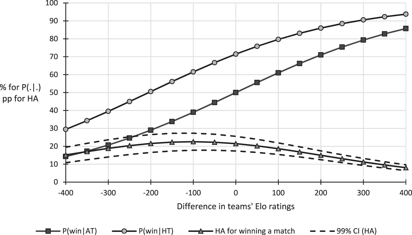
The probability of winning a match conditional on being a HT or being an AT, and HA for winning a match, by the teams’ difference in their Elo rating. Notes. HT, home team; AT, away team; HA, home advantage. The figure is for matches that cannot end in a draw. HA for winning a match = P(win|HT) − P(win|AT) where P(win|.) is the probability of winning a match conditional on being a HT or an AT. Based on Equations (1) and (2), and the estimation results in the third column of Table 4 (specification 3). Such a figure for matches that can end in a draw shows similar patterns.
3.3 Regression results of the model of Equation (3) and HA for tournament victory
On average, a HT had a higher probability of tournament victory than an AT and a team’s Elo rating had a positive effect on this probability (specification 1 of Table 5). In line with the finding in Table 4, there is no empirical support for HA in performance to vary with the HT’s Elo rating (specification 2 of Table 5). Furthermore, an increase in the number of participating teams reduced the probability of tournament victory and there is no empirical support for the number of matches played by the winner of the tournament affecting the probability of tournament victory. The latter finding is, arguably, related to a high correlation between the latter two variables of about 0.62 and without controlling for the number of participating teams, the number of matches played by the winner of the tournament has a significant negative effect (specification 3 of Table 5). Finally, there are no significant effects of interaction terms between playing at home and the number of teams, the number of matches played by the winner of the tournament, and team’s Elo rating in difference of the average Elo rating of teams (Table 5’s note), which supports the empirical specification.
Estimation results of a logistic model for the probability of tournament victory.
| Model specification | 1 | 2 | 3 | 4 |
|---|---|---|---|---|
| Coef. | Coef. | Coef. | Coef. | |
| (Std. err.) | (Std. err.) | (Std. err.) | (Std. err.) | |
| [p-value] | [p-value] | [p-value] | [p-value] | |
| # Participating teams | −0.056 | −0.056 | −0.048 | |
| (0.017) | (0.017) | (0.019) | ||
| [0.001] | [0.001] | [0.014] | ||
| # Matches of the winner | −0.079 | −0.079 | −0.273 | −0.136 |
| (0.086) | (0.086) | (0.067) | (0.102) | |
| [0.361] | [0.362] | [<0.001] | [0.184] | |
| HT/# hosts | 2.322 | 2.284 | 2.395 | 2.389 |
| (0.218) | (0.254) | (0.217) | (0.224) | |
| [<0.001] | [<0.001] | [<0.001] | [<0.001] | |
|
|
0.730 | 0.720 | 0.748 | 0.740 |
| (0.066) | (0.074) | (0.066) | (0.072) | |
| [<0.001] | [<0.001] | [<0.001] | [<0.001] | |
| HT/# hosts
|
0.050 | |||
| (0.172) | ||||
| [0.772] | ||||
| Constant | −2.017 | −2.001 | −1.710 | −1.873 |
| (0.406) | (0.410) | (0.397) | (0.447) | |
| [<0.001] | [<0.001] | [<0.001] | [<0.001] | |
| Pseudo R2 (McFadden 1974) | 0.269 | 0.269 | 0.259 | 0.284 |
| AUC (Bamber 1975) | 0.861 | 0.861 | 0.856 | 0.871 |
| Number of teams (observations) | 2002 | 2002 | 2002 | 1740 |
| Number of tournaments | 177 | 177 | 177 | 156 |
-
Notes. Sample: see Section 2 and Table 1. Specification 4: the sample is restricted to tournaments with a single host country. The estimates of α of Equation (3) are shown. HT is a binary variable equal to 1 if the team’s country hosted the tournament, and 0 otherwise. ‘# participating teams’ is the number of participating teams in a tournament (N in Equation (3)). ‘# hosts’ is the number of host countries of a tournament (NH in Equation (3)). ‘# matches of the winner’ is the number of matches the winner played at a tournament (G in Equation (3)).
For an average cup tournament, the probability of tournament victory was for a HT with an average Elo rating about 22 pp higher than if this team would not have played at home (Figure 2: 25.6 % vs. 3.3 % for
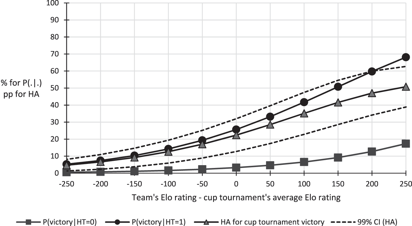
The probability of tournament victory conditional on being the HT or the AT, and HA for tournament victory by the team’s Elo rating in difference of the cup average. Notes. Home advantage (HA) for tournament victory = P(victory|HT = 1) − P(victory|HT = 0) where P(victory|.) is the probability of tournament victory conditional on HT equal to 0 or 1 (HT, home team; AT, away team). Based on Equations (3) and (4) with N = 16 and G = 6, for a cup tournament with a single host country (NH = 1), and the estimation results of specification 1 of Table 5.
![Figure 3:
The ratio of HA for tournament victory and HA for winning a match. Notes: HA, home advantage. ‘Extrapolation’ refers to HA for tournament victory being outside the [−250, 250] interval (Figure 2). ‘Difference in Elo ratings’ refers to ‘difference in teams’ Elo rating’ for the x-axis values of Figure 1 and to ‘Team’s Elo rating – cup tournament’s average Elo rating’ for the x-axis values of Figure 2. The ratios of the pp HA corresponding to these values in Figures 2 and 3 form the ‘Ratio’ curve in Figure 3 (HA for tournament victory/HA for winning a match).](/document/doi/10.1515/jqas-2024-0056/asset/graphic/j_jqas-2024-0056_fig_003.jpg)
The ratio of HA for tournament victory and HA for winning a match. Notes: HA, home advantage. ‘Extrapolation’ refers to HA for tournament victory being outside the [−250, 250] interval (Figure 2). ‘Difference in Elo ratings’ refers to ‘difference in teams’ Elo rating’ for the x-axis values of Figure 1 and to ‘Team’s Elo rating – cup tournament’s average Elo rating’ for the x-axis values of Figure 2. The ratios of the pp HA corresponding to these values in Figures 2 and 3 form the ‘Ratio’ curve in Figure 3 (HA for tournament victory/HA for winning a match).
Finally, Figure 3 shows HA for tournament victory relative to HA for winning a match. This relative difference is monotonically increasing in HT’s Elo rating, a finding in accordance with compound probability causing HA for tournament victory to increase with HT’s Elo rating (see Section 2.2.2).
3.4 World Cup host countries and HA: an illustrative example
The 2010 and 2014 FIFA World Cups can further illustrate the implications of our empirical findings. These World Cups were similar in terms of numbers of participating teams (32), matches played, and average Elo rating of teams (1,804 Elo points in 2010 and 1,842 Elo points in 2014). These two tournaments were, however, two extremes with respect to the HT’s strength: the 2010 World Cup was hosted by South Africa, whose team had a relatively low Elo rating (1,521 Elo points), while the 2014 tournament was hosted by Brazil, whose team had a relatively high Elo rating (2,132 Elo points).
Our findings of Table 4 suggest that the teams from South Africa and Brazil enjoyed a similar HA in performance. The predicted HA for winning a match against a team with an average Elo rating was higher for the South African team than for the Brazilian team (Figure 1). However, for a given opponent, and while having had HA, the South African team had a lower probability of winning a match than the Brazilian team (Figure 1) which, according to our results, caused the Brazilian team to have a higher predicted HA for tournament victory than the South African team did (Figure 2). However, because Figure 2 is not based on a cup tournament with 32 teams, but on one with 16 teams, it overstates the importance of HA for the South African and Brazilian teams. Therefore, the following comparison of the two World Cup cases accounts for 32 participating teams and that the winner of the tournament played seven matches. Based on the results of Table 5, by playing at home the predicted probability of tournament victory increased from 0.2 % to 1.6 % for the South African team and from 9.6 % to 51.9 % for the Brazilian team. That is, the Brazilian team is predicted to have had about a 41 pp higher HA for tournament victory than the South African team did (99 % CI: 22.3–58.7).
Hence, the host countries of these two World Cups can have mattered for the tournament outcomes of not only the South African and Brazilian teams but also for the outcomes of the ATs. That is, our findings suggest a lower expected disadvantage for tournament victory for an AT when South Africa hosted the tournament than when Brazil did.
3.5 Discussion of robustness analyses
Excluding tournaments with multiple host countries for the analysis did not affect the main findings (specification 4 of Table 5). Also, modelling the influence of multiple host countries by dividing HT by the number of host countries cannot be rejected against a specification with different HT effects for tournaments with a single host country, those with multiple host countries, and those that consisted solely of two-legged ties with home and away matches for which all countries were effectively host countries (a p-value of 0.843). Our model specification can also not be rejected against a specification that assumes no HT effect for tournaments that consisted solely of two-legged ties with home and away matches (a p-value of 0.891).
When using a linear probability model (LPM), hence without assuming a logistic distribution function when modelling win-probabilities (Equations (1) and (3)), the estimated marginal effects on the probability of winning a match and the probability of tournament victory are in accordance with those of Tables 4 and 5. Also, our main conclusion concerning the variation in HA for tournament victory by HT’s Elo rating remains when employing a LPM. A LPM can also be employed to assess the importance of measurement error in Elo ratings, e.g., because of underrating the hosts of major tournaments (Kaminski 2022), which would attenuate the predicted probabilities for given Elo ratings (Bound et al. 2001; Stefanski and Carroll 1985). While, based on instrumental variables estimation, there is evidence of measurement error in Elo ratings, the attenuation bias was found to be relatively small (about 10 %). Nevertheless, this study’s predicted variation in HA for tournament victory by HT’s Elo rating can be conservative.
Seeding can also affect variation in HA for tournament victory by HT’s strength because typically the HT is assigned to the first (strongest) pot independently of its strength when determining the playing schedule, hence avoids the strongest teams in the group stage (Lapré and Palazzolo 2023; Monks and Husch 2009). This issue was examined by estimating Equation (3) with only the 968 matches of the knockout stages. The reduced sample size caused less precise estimates and the size of HA for tournament victory is smaller because of fewer teams and fewer matches were played by the winner of the tournament (three on average). Nevertheless, we find for this subsample a similar pattern as the one in Figure 2: HA for tournament victory increases with HT’s Elo rating.
Further, HA can vary over time, by tournament stage, or by cup tournament (Allen and Jones 2014; Baker and McHale 2018; Clarke and Norman 1995; Lago-Peñas and Lago-Ballesteros 2011; Peeters and van Ours 2021; Pollard 2006; Pollard and Armatas 2017; Ramchandani et al. 2021). We found no empirical support for such variation in HA for tournament victory with the notable exception of suggestive evidence of a time effect in HA. For instance, the p-value for testing no variation in HA by cup tournament was 0.153 (seven groups considered: FIFA World Cups and the six continental championships). The p-value for testing no variation over time in HA for tournament victory was 0.043 and the point estimates suggest that HA was larger before 1971 and about the same for the periods 1971–1999 and 2000–2024. This may suggest the need for allowing HA to change over time when computing Elo ratings for national teams, like for the Elo ratings of European football clubs (http://clubelo.com/system).
Finally, the effects of being the HT on the probability of playing a semi-final or the final match are in accordance with the findings for HA for tournament victory. HA for a final ranking cannot be computed because there is no such ranking for all teams at a cup tournament.
4 Discussion
The main empirical findings support that HA for tournament victory can increase with an increase in HT’s Elo rating. The variation is also meaningful: On average, HA increased the probability of tournament victory from 3.3 % to 25.6 % for a HT with an average Elo rating, i.e., a HA for tournament victory of 22.4 pp (99 % CI: 12.7–32.0). HA increased to 41.6 pp (99 % CI: 28.6–54.6) for a HT with a one SD higher than average Elo rating and reduced to 9.2 pp (99 % CI: 3.8–14.7) for a HT with a one SD lower than average Elo rating. Furthermore, our findings support that the variation is in accordance with an important role for compound probability (Figure 3) and not because of HA in performance varying by HT’s Elo rating (specification 2 in Tables 4 and 5). These findings also imply that the average away disadvantage of ATs for tournament victory varied by HT’s Elo rating because there can only be one winner of the tournament.
4.1 Limitations and perspectives
Section 3.4 discussed HA for the South African and Brazilian teams at the 2010 and 2014 FIFA World Cups, respectively. As it turned out, the Brazilian team did not win the 2014 World Cup because it lost against the German team in the semifinal. The Brazilian team may have choked under the pressure of being favourite to win the tournament because the loss was severe, a 7 to 1 win for the German team. This exemplifies, that HA and Elo ratings explain only part of the variation in the outcomes of a cup tournament (see Table 5) and that future research is needed to shed light on the unexplained part.
As mentioned, factors such as choking under pressure or seeding may play a role in the variation in HA for tournament victory by HT’s strength (Baumeister and Steinhilber 1984; Jordet et al. 2012; Monks and Husch 2009). The possibility of HA varying by unobserved factors points toward the limitation that the main empirical findings are estimates of average HA effects. Future research can, e.g., assess the importance for HA for tournament victory of choking under pressure by using information on the experience or age of players and coaches.
Further, next to whether a team was a HT, the probability of tournament victory was approximated with the number of matches the winner of the tournament played, the number of participating teams, and a team’s Elo rating in difference from the average Elo rating of the participating teams. This approach can be considered a first step for empirical research on HA for cup tournament outcomes and future research can extend the analysis by, e.g., including information on the distribution of Elo ratings.
Finally, the quantifications of predicted outcomes for specific cup tournaments and teams are beyond this study’s scope. We presented in Figure 2 expected outcomes for an average cup tournament and in Section 3.5 for the 2010 and 2014 World Cups. There are various other tournament setups that can be studied using our estimation results. Also, future research can build on this study’s methods and findings and use more complex simulation models to also account for matters that are beyond the scope of this study, such as the playing schedule.
5 Conclusions
Our findings support that the country in which a cup tournament is played can, through the HT’s strength, have meaningful effects on the tournament outcomes of all participating teams and not only on the outcome of the HT. That is, also the outcome for an AT can be affected by where the cup tournament is played. HA can, therefore, substantially worsen the efficacy of cup tournaments and can be a factor to consider in studies on tournament design (Lasek and Gagolewski 2018; McGarry and Schutz 1997; Sziklai et al. 2022) and on the slot allocation method in the FIFA World Cup, i.e., the number of participating teams from each continent in the final tournament (Csató et al. 2024; Krumer and Moreno-Ternero 2023).
Finally, HA for tournament outcomes is a feature of cup tournaments with a single host country or multiple host countries. Such a tournament setup can, e.g., have entertainment value, increase interest in the game of football in a host country and have logistical advantages. Nevertheless, the impact of the decision which country will host a cup tournament on tournament outcomes could be a factor to consider by a tournament organiser when deciding on which bid for hosting the tournament to accept.
Acknowledgments
I am very grateful for the comments and feedback received from the participants of the seminar given at Utrecht University School of Economics.
-
Research ethics: This study has been approved by the Ethics Committee of the Faculty of Law, Economics and Governance at Utrecht University.
-
Informed consent: Not applicable.
-
Author contributions: The author has accepted responsibility for the entire content of this manuscript and approved its submission.
-
Use of Large Language Models, AI and Machine Learning Tools: None declared.
-
Conflict of interest: The author states no conflict of interest.
-
Research funding: None declared.
-
Data availability: The data are available from various public online sources (Appendix A.2).
Appendices A.1 Compound probability and HA for tournament victory by HT’s strength
Consider a tournament with four teams (one HT and three ATs) and two elimination rounds. A match is between two teams and ends in a win or a loss. The first-round winners play in the second round the final match for tournament victory. The ATs all have a strength equal to 1 and the strength of the HT is α (α > 0). HA in performance is h (h > 0). The probability that the HT wins a match is
A.2 Data sources
The Elo ratings of national football teams are available from the World Football Elo Ratings (www.eloratings.net). The FIFA rankings of national teams since 1992 are available from www.fifa.com. Since 2018 the FIFA rankings are based on an Elo system. The ratings and rankings used for this study are valid on December 31 of each calendar.
The results of matches played by national football teams at FIFA World Cups and at the championships for national teams organized by the six FIFA-affiliated continental confederations are publicly available from the following websites:
https://en.wikipedia.org/wiki/AFC_Asian_Cup (AFC: Asian Football Confederation; AFC Asian Cup),
https://en.wikipedia.org/wiki/Africa_Cup_of_Nations (CAF: Confédération Africaine de Football; Africa Cup of Nations),
https://en.wikipedia.org/wiki/CONCACAF_Gold_Cup (CONCACAF: Confederation of North, Central American and Caribbean Association Football; CONCACAF Gold Cup),
https://en.wikipedia.org/wiki/Copa_America (CONMEBOL: Confederación Sudamericana de Fútbol – Copa América),
https://en.wikipedia.org/wiki/OFC_Nations_Cup (OFC: Oceania Football Confederation – OFC Nations Cup),
https://en.wikipedia.org/wiki/UEFA_European_Championship (UEFA: Union of European Football Associations – UEFA European Football Championship),
https://en.wikipedia.org/wiki/FIFA_World_Cup (FIFA: Fédération Internationale de Football Association – FIFA World Cup).
The CONCACAF Gold Cup is formally known as the CONCACAF Championship, the CONMEBOL Copa América as the South American Football Championship, the OFC Nations Cup as the Oceania Cup, and the UEFA European Football Championship as the European Nations’ Cup. The national teams are members of one of the six continental confederations (AFC, CAF, CONCACAF, CONMEBOL, OFC or UEFA). Also, teams can switch from confederation (e.g., Australia). Furthermore, FIFA guidelines are followed when national teams have merged, and one of the teams ceased to exist, or split and new teams were formed.
References
Allen, M.S. and Jones, M.V. (2014). The home advantage over the first 20 seasons of the English premier league: effects of shirt colour, team ability and time trends. Int. J. Sport Exerc. Psychol. 12: 10–18, https://doi.org/10.1080/1612197x.2012.756230.Search in Google Scholar
Baker, R.D. and McHale, I.G. (2018). Time-varying ratings for international football teams. Eur. J. Oper. Res. 267: 659–666, https://doi.org/10.1016/j.ejor.2017.11.042.Search in Google Scholar
Bamber, D. (1975). The area above the ordinal dominance graph and the area below the receiver operating characteristic graph. J. Math. Psychol. 12: 387–415, https://doi.org/10.1016/0022-2496(75)90001-2.Search in Google Scholar
Baumeister, R.F. and Steinhilber, A. (1984). Paradoxical effects of supportive audiences on performance under pressure: the home field disadvantages in sports championships. J. Pers. Soc. Psychol. 47: 85–93, https://doi.org/10.1037/0022-3514.47.1.85.Search in Google Scholar
Benjamin, D.J. and Berger, J.O. (2019). Three recommendations for improving the use of p-values. Am. Stat. 73: 186–191, https://doi.org/10.1080/00031305.2018.1543135.Search in Google Scholar
Benjamin, D.J., Berger, J.O., Johannesson, M., Nosek, B.A., Wagenmakers, E.J., Berk, R., Bollen, K.A., Brembs, B., Brown, L., Camerer, C., et al.. (2018). Redefine statistical significance. Nat. Hum. Behav. 2: 6–10, https://doi.org/10.1038/s41562-017-0189-z.Search in Google Scholar PubMed
Bound, J., Brown, C., and Mathiowetz, N. (2001) Measurement error in survey data, Ch. 59. In: Heckman, J.J., and Leamer, E.E. (Eds.), Handbook of econometrics. Elsevier, Amsterdam, pp. 3705–3843.10.1016/S1573-4412(01)05012-7Search in Google Scholar
BrownJrT.D., Van Raalte, J.L., Brewer, B.W., Winter, C.R., Cornelius, A.E., and Andersen, M.B. (2002). World cup soccer home advantage. J. Sport Behav. 25: 134–144.Search in Google Scholar
Bryson, A., Dolton, P., Reade, J.J., Schreyer, D., and Singleton, C. (2021). Causal effects of an absent crowd on performances and refereeing decisions during Covid-19. Econ. Lett. 198: 109664, https://doi.org/10.1016/j.econlet.2020.109664.Search in Google Scholar
Chater, M., Arrondel, L., Gayant, J.-P., and Laslier, J.-F. (2021). Fixing match-fixing: optimal schedules to promote competitiveness. Eur. J. Oper. Res. 294: 673–683.10.1016/j.ejor.2021.02.006Search in Google Scholar
Clarke, S.R. and Norman, J.M. (1995). Home ground advantage of individual clubs in English soccer. Statistician 44: 509–521, https://doi.org/10.2307/2348899.Search in Google Scholar
Coates, D. and Humphreys, B.R. (2008). Do economists reach a conclusion on subsidies for sports franchises, stadiums, and mega-events? Working papers 08-18, international association of sports economists. North American Association of Sports Economists.Search in Google Scholar
Csató, L. (2023a). Group draw with unknown qualified teams: a lesson from 2022 FIFA World Cup. Int. J. Sports Sci. Coach. 18: 539–551, https://doi.org/10.1177/17479541221108799.Search in Google Scholar
Csató, L. (2023b). Quantifying the unfairness of the 2018 FIFA world cup qualification. Int. J. Sports Sci. Coach. 18: 183–196, https://doi.org/10.1177/17479541211073455.Search in Google Scholar
Csató, L. (2024). Club coefficients in the UEFA champions league: time for shift to an elo-based formula. Int. J. Perform. Anal. Sport 24: 119–134, https://doi.org/10.1080/24748668.2023.2274221.Search in Google Scholar
Csató, L., Kiss, L.M., and Szádoczki, Zs. (2024). The allocation of FIFA World Cup slots based on the ranking of confederations. Ann. Oper. Res. 344: 153–173.10.1007/s10479-024-06091-5Search in Google Scholar
Depetris-Chauvin, E., Durante, R., and Campante, F. (2020). Building nations through shared experiences: evidence from African football. Am. Econ. Rev. 110: 1572–1602, https://doi.org/10.1257/aer.20180805.Search in Google Scholar
Dowie, J. (1982). Why Spain should win the world cup. New Sci. 94: 693–695.Search in Google Scholar
Elo, A.E. (1978). The Rating of chess players, past & present. Second printing (2008). Ishi Press International, Bronx, NY.Search in Google Scholar
Falter, J.-M., Pérignon, C., and Vercruysse, O. (2008). Impact of overwhelming joy on consumer demand: the case of a soccer World Cup victory. J. Sports Econ. 9: 20–42, https://doi.org/10.1177/1527002506296548.Search in Google Scholar
Gásquez, R. and Royuela, V. (2016). The determinants of international football success: a panel data analysis of the Elo rating. Soc. Sci. Q. 97: 125–141, https://doi.org/10.1111/ssqu.12262.Search in Google Scholar
Gómez-Ruano, M.A., Pollard, R., and Lago-Peñas, C. (2022). Home advantage in sport: causes and the effect on performance. Routledge, New York, NY.10.4324/9781003081456Search in Google Scholar
Jia, H., Skaperdas, S., and Vaidya, S. (2013). Contest functions: theoretical foundations and issues in estimation. Int. J. Ind. Organ. 31: 211–222, https://doi.org/10.1016/j.ijindorg.2012.06.007.Search in Google Scholar
Jordet, G., Hartman, E., and Vuijk, P.J. (2012). Team history and choking under pressure in major soccer penalty shootouts. Br. J. Psychol. 103: 268–283, https://doi.org/10.1111/j.2044-8295.2011.02071.x.Search in Google Scholar PubMed
Kaminski, M.M. (2022). How strong are soccer teams? The “host paradox” and other counterintuitive properties of FIFA’s former ranking system. Games 13: 22, https://doi.org/10.3390/g13020022.Search in Google Scholar
Kooreman, P. and Schoonbeek, L. (1997). The specification of the probability functions in Tullock’s rent-seeking contest. Econ. Lett. 56: 59–61, https://doi.org/10.1016/s0165-1765(97)00131-6.Search in Google Scholar
Krumer, A. and Moreno-Ternero, J. (2023). The allocation of additional slots for the FIFA World Cup. J. Sports Econ. 24: 831–850, https://doi.org/10.1177/15270025231160757.Search in Google Scholar
Lago-Peñas, C. and Lago-Ballesteros, J. (2011). Game location and team quality effects on performance profiles in professional soccer. J. Sports Sci. Med. 10: 465–471.Search in Google Scholar
Lapré, M.A. and Palazzolo, E.M. (2022). Quantifying the impact of imbalanced groups in FIFA Women’s World Cup tournaments 1991–2019. J. Quant. Anal. Sports 18: 187–199, https://doi.org/10.1515/jqas-2021-0052.Search in Google Scholar
Lapré, M.A. and Palazzolo, E.M. (2023). The evolution of seeding systems and the impact of imbalanced groups in FIFA Men’s World Cup tournaments 1954–2022. J. Quant. Anal. Sports 19: 317–332, https://doi.org/10.1515/jqas-2022-0087.Search in Google Scholar
Lasek, J. and Gagolewski, M. (2018). The efficacy of league formats in ranking teams. Stat. Model. 18: 411–435, https://doi.org/10.1177/1471082x18798426.Search in Google Scholar
Lazear, E.P. and Rosen, S. (1981). Rank-order tournaments as optimum labor contract. J. Political Econ. 89: 841–864, https://doi.org/10.1086/261010.Search in Google Scholar
McFadden, D. (1974) Conditional logit analysis of qualitative choice behavior. In: Zarembka, P. (Ed.), Frontiers in econometrics. Academic Press, pp. 105–142.Search in Google Scholar
McGarry, T. and Schutz, R.W. (1997). Efficacy of traditional sport tournament structures. J. Oper. Res. Soc. 48: 65–74, https://doi.org/10.1038/sj.jors.2600330.Search in Google Scholar
Mitchell, H. and Stewart, M.F. (2015). What should you pay to host a party? An economic analysis of hosting sports mega-events. Appl. Econ. 47: 1550–1561, https://doi.org/10.1080/00036846.2014.1000522.Search in Google Scholar
Monks, J. and Husch, J. (2009). The impact of seeding, home continent, and hosting on FIFA World Cup results. J. Sports Econ. 10: 391–408, https://doi.org/10.1177/1527002508328757.Search in Google Scholar
Nalebuff, B.J. and Stiglitz, J.E. (1983). Prizes and incentives: towards a general theory of compensation and competition. Bell J. Econ. 14: 21–43, https://doi.org/10.2307/3003535.Search in Google Scholar
Nitzan, S. (1994). Modeling rent seeking contests. Eur. J. Political Econ. 10: 41–60, https://doi.org/10.1016/0176-2680(94)90061-2.Search in Google Scholar
Peeters, T. and van Ours, J. (2021). Seasonal home advantage in English professional football; 1974-2018. De Economist 169: 107–126, https://doi.org/10.1007/s10645-020-09372-z.Search in Google Scholar
Pollard, R. (2006). Worldwide regional variation in home advantage in association football. J. Sports Sci. 24: 231–240, https://doi.org/10.1080/02640410500141836.Search in Google Scholar PubMed
Pollard, R. (2008). Home advantage in football: a current review of an unsolved puzzle. Open Sports Sci. J. 1: 12–14, https://doi.org/10.2174/1875399x00801010012.Search in Google Scholar
Pollard, R. and Armatas, V. (2017). Factors affecting home advantage in football World Cup qualification. Int. J. Perform. Anal. Sport 17: 121–135, https://doi.org/10.1080/24748668.2017.1304031.Search in Google Scholar
Ramchandani, G., Millar, R., and Darryl, W. (2021). The relationship between team ability and home advantage in the English football league system. Ger. J. Exerc. Sport Res. 51: 354–361, https://doi.org/10.1007/s12662-021-00721-x.Search in Google Scholar PubMed PubMed Central
Rewilak, J. (2021). The (non) determinants of Olympic success. J. Sports Econ. 22: 546–570, https://doi.org/10.1177/1527002521992833.Search in Google Scholar
Schwartz, B. and Barsky, S.F. (1977). The home advantage. Soc. Forces 55: 641–661.10.2307/2577461Search in Google Scholar
Staufenbiel, K., Lobinger, B., and Strauss, B. (2015). Home advantage in soccer – a matter of expectations, goal setting and tactical decisions of coaches? J. Sports Sci. 33: 1932–1941, https://doi.org/10.1080/02640414.2015.1018929.Search in Google Scholar PubMed
Stefanski, L.A. and Carroll, R.J. (1985). Covariate measurement error in logistic regression. Ann. Stat. 13: 1335–1351, https://doi.org/10.1214/aos/1176349741.Search in Google Scholar
Stronka, W. (2024). Demonstration of the collusion risk mitigation effect of random tie-breaking and dynamic scheduling. Sports Econ. Rev. 5: 100025, https://doi.org/10.1016/j.serev.2024.100025.Search in Google Scholar
Szczecinski, L. and Roatis, I.-I. (2022). FIFA ranking: evaluation and path forward. J. Sport Anal. 8: 231–250, https://doi.org/10.3233/jsa-200619.Search in Google Scholar
Sziklai, B.R., Biró, P., and Csató, L. (2022). The efficacy of tournament designs. Comput. Oper. Res. 144: 105821, https://doi.org/10.1016/j.cor.2022.105821.Search in Google Scholar
Szymanski, S. and Drut, B. (2020). The private benefit of public funding: the FIFA World Cup, UEFA European Championship, and attendance at host country league soccer. J. Sports Econ. 21: 723–745, https://doi.org/10.1177/1527002520923701.Search in Google Scholar
Torgler, B. (2004). The economics of the FIFA football Worldcup. Kyklos 57: 287–300, https://doi.org/10.1111/j.0023-5962.2004.00255.x.Search in Google Scholar
Tullock, G. (1980) Efficient rent seeking. In: Buchanan, J., Tolliso, R., and Tullock, G. (Eds.), Towards a theory of the rent-seeking society. Texas A&M University Press, College Station, pp. 97–112.Search in Google Scholar
Wooldridge, J.M. (2010). Econometric analysis of cross section and panel data. MIT Press, Cambridge, Massachusetts, United States of America.Search in Google Scholar
© 2025 the author(s), published by De Gruyter, Berlin/Boston
This work is licensed under the Creative Commons Attribution 4.0 International License.