A network diffusion ranking family that includes the methods of Markov, Massey, and Colley
-
Stephen Devlin


Abstract
We present a one parameter family of ratings and rankings that includes the Markov method, as well as the methods of Colley and Massey as particular cases. The rankings are based on a natural network diffusion process that unites the methodologies above in a common framework and brings strong intuition to how and why they differ. We also explore the behavior of the ranking family using both real and simulated data.
1 Introduction
Ranking items based on objective criteria is a natural problem with a rich history of diverse applications (Kendall and Smith 1940; Langville and Meyer 2012). A particular application that has garnered much attention is the ranking of teams or players in sports. The nature of some sports, like NCAA football and basketball, with a small season of games relative to the number of teams involved, poses interesting challenges with respect to rankings. In these so-called uneven paired competitions, we are charged with ranking teams, often without the benefit of head-to-head results or even common opponents between teams. Running the gamut in a weak conference, for instance, is arguably less indicative of an exceptional team than is a season with only a few losses in an elite conference. Naturally, mathematical approaches to the ranking problem have been developed and adopted in various contexts (Stefani 2011).
Our focus is three of the most well-known and widely studied ranking methodologies in sports: Massey’s method (Massey 1997), Colley’s method (Colley 2002), and the Markov method. The methods of Massey and Colley were both ingredients in the BCS rankings in college football, while the Markov method serves as the foundation for Google’s PageRank algorithm.
While the similarities between the methods – especially those of Colley and Massey – have been extensively noted, less has been written about why these approaches, each with their own distinct motivations, result in such similar linear systems. Since the ranking problem is a fundamentally unsupervised one – there is no ground truth against which to evaluate outcomes – a sound intuition for how methods are similar and how they differ is especially important in comparing results and choosing an approach to a particular application. One important tool that is widely used in comparing ranking methods is based on an axiomatic approach. Here, desirable properties of a ranking methodology are laid out explicitly as axioms, and proposed methodologies are compared with respect to how they satisfy or violate these axioms. Many of the ranking methods we discuss here are explored in this way in González-Díaz, Hendrickx, and Lohmann (2014) and Vaziri et al. (2018).
In this paper we present an intuitive, unifying framework in which to understand the ranking methods of Colley, Massey, and Markov. Our entry point is a simple diffusion process on a network. Using this process we define a family of rankings that depends on a single, natural parameter, and show that this family effectively interpolates between the methodologies above. This helps bring insight to how each of the methodologies processes input information, and clarifies the underlying similarities and differences. Moreover, the family of methods defined provides context and intuition for choosing a ranking methodology based on objective a priori criteria rather than simply the observed result of the rankings themselves. We also explore the resulting rankings and the extent to which they agree and disagree with detailed examples on both real and simulated data.
2 Ranking methods
2.1 Massey
Massey’s method was introduced by Kenneth Massey in Massey (1997). The method is based on the premise that the difference in two teams’ ranks should predict the point differential in a game between those teams. If we wish to rank n teams involved in m games, we get a linear system,
where r is the desired rating vector in ℝn, and y is a vector of point differentials whereby the k-th component of y is the true point difference in game k. The only nonzero entries in the k-th row of X are a −1 in the column of the winning team, i, and a -1 in the column of the losing team, j. The matrix X is m × n. Since m is larger than n in practice, the system will almost always be inconsistent and Massey proceeds via the usual least-squares approach:
Let M = XTX and let p = XTy. If nij is the number of games between teams i and j and Ni is the total number of games played by team i, then the matrix M has the following form:
The vector p gives the aggregate point differential over all games for each team. Massey’s system,
however, is rank deficient (the rows of M all sum to 0). As a final fix, Massey replaces the last row of M with a row of ones, and similarly replaces the last entry of p with 0. This forces the ratings to sum to zero and gives the modified system, M′r = p′, a unique solution. We note that the same end can be achieved by simply augmenting the Massey system in (4) to the block system
thus forcing the ratings to sum to zero in the same way. If point differentials are unknown or unwanted (as was the case in the BCS ranking that prohibited the use of point information), a vector based on wins and losses can be substituted for the point differential vector p in (4). Making this substitution also facilitates comparisons with methodologies that do not use score information as we will see below. We also note that this version of Massey’s method with wins and losses in place of point differentials has a long history that predates Massey’s approach and is commonly referred to as the least squares ranking method. See, for instance, the work of Horst (1932); Mosteller (1951), and for more recent work, Csató (2015).
One note on notation moving forward: We distinguish between the rating vector r, which assigns a numerical value to each team, and the resulting ranking, a permutation of 1, 2, … n, that r determines. For a ranking, we specify that team team j is ranked above team i, and write i ⪯ j whenever ri ≤ rj. If the context is clear, we can refer to the ranking r as the ranking ⪯ determined by the rating vector r.
2.2 Colley
Colley’s method is introduced in Colley (2002). Colley uses a modified winning percentage of the form
with
and
Note that despite their different motivations, Colley and Massey arrive at remarkably similar matrices. Letting I be the n × n identity matrix, we have C = 2I + M, an identity we return to below.
2.3 Markov
Markov chain methods are highly adaptable and find a wide range of applications (Von Hilgers and Langville 2006). For ranking, one of the most well-known applications is the Google PageRank algorithm (Brin and Page 1998). Markov based methods are often tailored to a variety of applications in sports, including work in Kvam and Sokol (2006); Mattingly and Murphy (2010); Callaghan et al. (2007). We consider an implementation of a Markov ranking that is particularly natural in the context of ranking teams.
Let each team be represented by a node in a network with edges between teams that play one another. Let wij be the number of wins for team i against team j when i ≠ j, and let Wi be the total number of wins for team i. Define a random walk on the nodes (teams) of the network where the walker moves from team j to team i with probability proportional to the number of times that i beat j, and stays put at team i with probability proportional to the total number of wins accumulated by team i. The n × n transition matrix T for this walk is given by:
The Markov rating r is a stable solution to Tr = r. That is, r is an eigenvector of T corresponding to the eigenvalue λ = 1. The vector r can be interpreted as giving the long-term probability that the walker is at each node in the network. Since T is column stochastic, such a nonzero positive eigenvector is guaranteed to exist under mild assumptions. For instance, we cannot have a winless team (a row of zeros in T), or two groups of teams where one group always beats the teams in the other. Those familiar with the PageRank algorithm will recognize these problems and recall that they can be remedied by repairing dangling nodes and using a teleportation matrix, but for simplicity we will consider only the case where T is irreducible.
If we let
and introduce the diagonal matrix
then the Markov rating satisfies GN−1r = r, or equivalently,
The matrix N − G has the form:
where Li is the number of losses for team i. In order to compare teams having potentially played different numbers of games, we normalize r by the number of games played, and take the vector v = N−1r as the rating vector. This replaces the fraction of time spent at i, with the fraction of time spent at i per edge of i, a value that can be readily compared across nodes. Equation (10) then becomes
3 Diffusion
3.1 Graph diffusion I
Building on the notation in Section 2.3, suppose the nodes of an undirected network have been labeled from 1 to N. Following Newman (2010), we define a discretized diffusion process on the network as follows. Suppose that a fixed quantity of a substance that we call rank, thought of as a gas or liquid, is distributed over the nodes of the network. At each time step, we allow a quantity of rank to move along the network’s edges. We dictate the physics of the system so that rank flows from higher pressure nodes to lower pressure nodes. In one time step, therefore, we specify that the quantity of rank flowing from node j to node i is proportional to the difference in the rank at those nodes. Let vt be the vector whose i-th component
where k is called the diffusion constant, and Aij is the entry in the i-th row, j-th column of the adjacency matrix, indicating whether or not there is an edge between i and j that would allow rank to flow. Expanding the sum we can write:
where δij is the Kronecker delta,
and di = ∑jAij is the degree of vertex i.
Asking that the long-term net change in rank be zero for all nodes, Equation (15) leads to the matrix equation
where D is the diagonal matrix whose i-th diagonal entry is the degree of node i, and v is called a stable solution (or equilibrium). The matrix (D − A) is the well-known graph Laplacian (Cvetkovic, Doob, and Sachs 1980). The continuous version of (15) yields a differential equation governing the rate of flow between nodes of the network, which is solvable in closed form in terms of the eigenvalues of the Laplacian.
3.2 Graph diffusion II and the Markov ranking
Next consider a variant of the above diffusion process where the network is weighted and directed. Assume that for i ≠ j the fraction of rank-flow from vertex j to vertex i is proportional to given weights bij. The total weighted degree of vertex i, or total flow through i, is given by
where
Finally, we specify that rank that does not flow out of vertex i stays at i, and set Bi = din(i). A stable solution to this diffusion process is then a rating vector r such that the total flow into vertex i is equal to the flow out of i. Thus, for each i,
If we let B be the weighted adjacency matrix with (i, j)-entry equal to bij for i ≠ j and Bi for i = j, and let N be the diagonal matrix with Ni on the diagonal in the i-th row, the system of equations defined by (20) gives the matrix equation:
The matrix (N − B) is a weighted version of the graph Laplacian of (18) on the directed network, and (21) again asks that the net change in rank be zero at all vertices. Setting v = N−1r, we write (21) as
Note that (21) and (22) take precisely the same form as (10) and (12). The Markov ranking, therefore, especially the form in (12), is equivalent to a diffusion process on the connection network of teams. This equivalence between a random walk (Markov process) and a diffusion process is well known (Newman 2010). Here, the fraction of flow into team i from team j is given by the number of wins i has against j, and the flow out of i is given by the total number of losses. Equation (12) asks that the net flow through all vertices be zero. Also note that the net-flow-zero solution is given, as in (18), by a vector in the nullspace of the associated graph Laplacian.
3.3 A one parameter ranking family
Given the equivalence of the Markov rating of (12) and the diffusion process of (22), we define a family of rankings that depends on a single parameter and has a natural interpretation as a diffusion process. Suppose there are n teams to rank, and define win and loss matrices
and
where wij and lij are, respectively, the number of wins and losses for team i against team j, and Wi and Li are the total number of wins and losses for team i. For p a parameter with 0 ≤ p ≤ 1, define
and take
We begin by trying to define a rating vector vp as a solution to
When p = 0, note that we get precisely the Markov equation in (12), or equivalently, the net-flow-zero equation of (22). Requiring that x = v0 be a probability vector, therefore, recovers the Markov rating when p = 0.
Also note that for p > 0, any rating vector satisfying (27) will be a scalar multiple of a rating vector satisfying ℒpx = s. From the perspective of the underlying ranking problem, therefore, we can define
and rewrite (27) as
Finally, note that when p > 0 the columns of ℒp are still linearly dependent, so a constraint is still required to identify a rating vector. While the particular constraint choosen is irrelevant from the perspective of the resulting ranking, we follow the common convention [and the one used in (5)] that the rankings sum to 0:
Thus, taking x = vp to be the rating vector solving (30), and letting
For p > 0, the system (31) is still interpreted using the diffusion paradigm of Section 3.2. As before, the (i, j)-entry of the matrix ℒp represents the flow from j to i [compare with the left hand side of (22)]. Now, however, the flow is not determined solely by wins for i versus j. Indeed, in this more generous process even losses to team j contribute some flow to team i as regulated by the parameter p. Thus, increasing p from 0 moves the diffusion process away from a pure meritocracy, toward a ranking where teams get some credit for simply playing against other teams, and especially for playing against other good teams (with high rankings). As p grows we weaken the importance of the result of the interaction between teams from the perspective of rank flow. To compensate, we introduce a measure of overall team success based on aggregate outcomes and represented by the vector sp on the right hand side of (31). Continuing the diffusion analogy, the vector sp represents an external infusion of rank (possibly negative) at each vertex i.
The particular choice for the infusion of rank here is a win percentage proxy given by wins minus losses, though there is no reason why other choices could not be made. (Massey’s original method, for example, uses cumulative point differential and would be a natural choice.) The rank infusion vector can be considered an external success metric in that it is not network dependent: two teams with the same record will get the same infusion regardless of which teams they played. The network dependent rank-flow update to sp is given by the left-hand-side of (31). With this s, note that the rankings obtained by solving ℒ0x = 0 in the Markov method are the same as the rankings from solving ℒ0x = s (though the ratings are different). This is specific, however, to this particular choice of s and wouldn’t hold for other infusion vectors like Massey’s point differential. The choice of infusion used here will clarify the connection with Colley’s and Massey’s methods as seen below, while still giving a continuous family of ratings. Finally, we also note that the ranking problem as described here bears a strong resemblance to problems of current flow on electrical networks as described in Doyle and Snell (2000).
4 Connections
The connection between the diffusion ranking with p = 0, ℒ0, and the Markov ranking is already established. Now take p = 1 and consider the diffusion ranking
With flow from losses turned fully on, a win and a loss are of equal value with respect to rank-flow. Thus, the head-to-head results of games are relevant only in that they occurred, and provide a strength-of-schedule update to the rank-infusion vector s1 as determined by the team’s overall aggregate record. Furthermore, note that ℒ1 = M: The rank-diffusion Laplacian ℒ1 is precisely the Massey matrix M in (3). On the other hand, the right-hand-side vector s1 is related to the Colley right-hand-side b from (6) by
As noted earlier, the Colley matrix C satisfies C = 2I + M, where M is the Massey matrix. The Colley rating r in (6) can thus be written
or in our new notation
Leaving behind Colley’s original motivation, the 2I on the left hand side of (33) and the 1 on the right serve the two-fold purpose of making the Colley matrix invertible and normalizing the ratings so that they have an average value of
also gives a rating where the average value is
A natural choice in light of the diffusion interpretation would be to not manipulate the rank-flow at all, and let k = 0. Doing so (and dropping the
It is worth making note of another interpretation for Colley’s method. Though not part of his original presentation, Colley’s rating can be recast as a regularized regression by applying a ridge penalty to the Massey matrix X in (1). See Glickman and Stern (2017) for details. The parameter that controls the regularization penalty here is the 2 on the left hand side of (33), though usually this parameter is chosen in a more rigorous way via cross validation. We address validation of both the choices of k in (35) and p in (31) below.
The modified Colley (m-Colley) method of (36) with k = 0, and the Massey method, differ only in their choice of normalization of the ranking vector, and their choice of the right-hand-side. Obviously the choice of the right-hand-side infusion vector is a fundamental one. If for purposes of comparison, however, we choose the same right-hand-side s1 from (26) then the methods are, in fact, identical.
One can also consider the so-called Colleyized Massey (C-Massey) method where the Colley right hand side is used in place of point-differentials along with Massey’s Matrix (Langville and Meyer 2012). In light of the discussion above, one might prefer to use s1, the m-Colley right-hand-side (taking k = 0) for the infusion vector.
In the notation of (32) this can all be summarized as follows:
where we consider the +1 on the right hand side of (38) as optional depending on the form of Colley’s method you choose to consider.
5 Examples
In order to explore the behavior of the
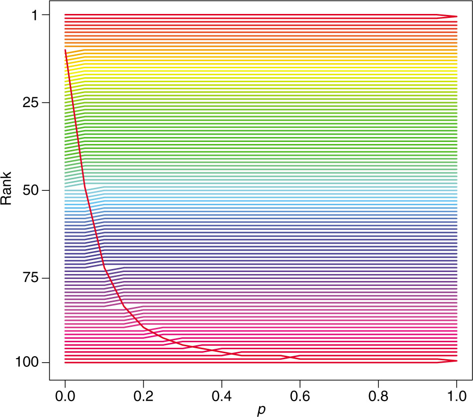
Rankings in a perfect season with maximal worst-beats-best upset. Each team is represented by a fixed color, and it’s rank is plotted across values of p ranging from p = 0 (Markov) to p = 1 (m-Colley/Massey).
We show the results for n = 100 teams in Figure 1 with p running from 0 to 1 in steps of 0.10. In this case, the original Colley method (not pictured) of (6) results in a change in ranking for the first two and last two teams, respectively. The no-longer undefeated team drops into a tie for first place with the formerly second ranked team while the formerly winless team now rises into a tie with the formerly penultimate team. Similarly the m-Colley (k = 0) method (or Colleyized-Massey method) also results in a tie between both the top two and bottom two teams. This is consistent with the intuition developed above. Since Colley and Massey (without point differentials in the RHS) only consider game outcomes in the aggregate of wins and losses, and otherwise inform ratings using who-played-whom strength of schedule (losses are turned fully on in the diffusion), the top two teams (resp. bottom two teams) have the same record and the same schedule, so there is no other basis by which to differentiate them. A more rigorous explanation for this would invoke Proposition 5.3 of González-Díaz et al. (2014), and note that since the p = 1 ranker satisfies the score consistency axiom of agreeing with the ranking from winning percentages on round robin tournaments, the resulting ranking must follow.
By contrast, the Markov method results in the formerly winless team rising all the way to 11th, with all teams formerly ranked 11 or below dropping one place to accommodate the change. The example also clearly shows that the behavior of Markov and Colley/Massey reflect the respective extremes of a continuum of results parameterized by p and given by the appropriate rating of (31). As p increases from zero (Markov), the formerly last ranked team, having upset the top team, drops quickly in the rankings. By p = 0.20 it has dropped from 11th (p = 0) to 90th. This raises an interesting and debatable question of how much the bottom team should be rewarded for an upset of this magnitude. While stability of a ranking methodology is indeed attractive, there is a philosophical appeal to rewarding teams for beating the best opponents, at least to some extent. See, for example, property 1 in Vaziri et al. (2018). Intermediate values of p allow for a measure of compromise. We consider a more principled approach for choosing p by optimizing the prediction accuracy of the ratings below.
The properties of the rating vectors as they pertain to the stability of the actual rankings in the three methods was discussed in detail in Chartier et al. (2011). In particular, while the Massey and Colley methods produce ratings in the perfect season that are equally spaced and highly stable, the Markov rating vector is highly non-uniform in it’s distribution of values (and hence far less stable in the face of perturbations). In Figure 2 we show that these properties also represent extremes in a continuum of behaviors, with ratings becoming more and more evenly spaced as p increases from 0 until we arrive at the uniform spacing of p = 1.
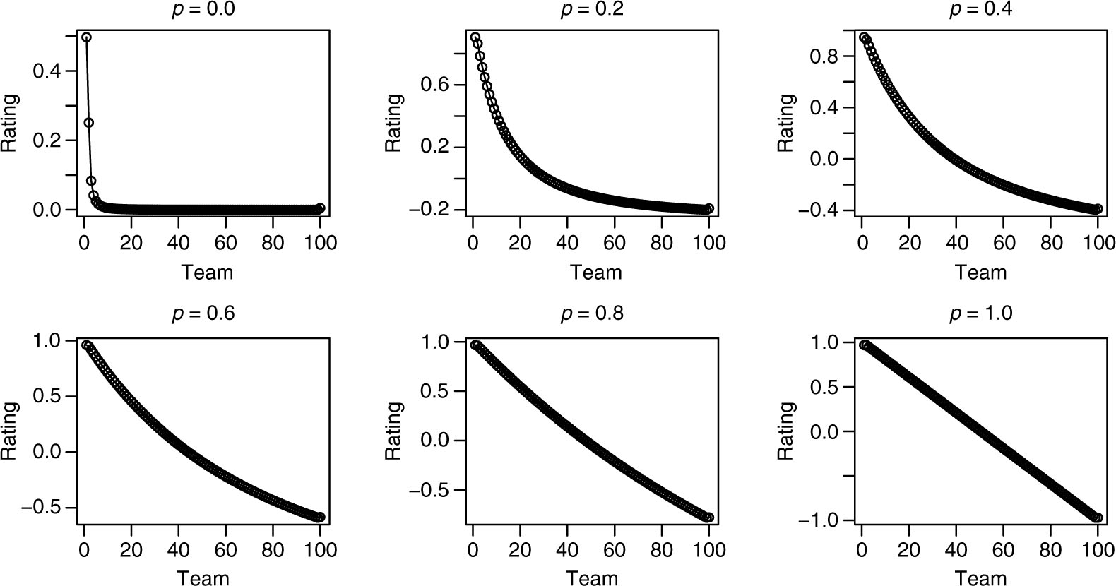
Values of the rating vector for given values of the parameter p in Equation (40), and applied to the perfect season with upset.
Sample rankings for 2016–2017 men’s NCAA division one college basketball.
| Team | p | ||||||||||
|---|---|---|---|---|---|---|---|---|---|---|---|
| 0.0 | 0.10 | 0.20 | 0.30 | 0.40 | 0.50 | 0.60 | 0.70 | 0.80 | 0.90 | 1.0 | |
| Gonzaga | 1 | 2 | 3 | 3 | 3 | 4 | 5 | 6 | 7 | 7 | 7 |
| Villanova | 2 | 1 | 1 | 1 | 1 | 1 | 1 | 1 | 1 | 1 | 1 |
| Kansas | 3 | 3 | 2 | 2 | 2 | 2 | 2 | 2 | 2 | 2 | 2 |
| Butler | 4 | 4 | 7 | 9 | 9 | 11 | 12 | 12 | 13 | 14 | 14 |
| Arizona | 5 | 5 | 4 | 4 | 5 | 5 | 4 | 4 | 4 | 4 | 4 |
| UCLA | 6 | 6 | 8 | 8 | 8 | 8 | 8 | 8 | 9 | 10 | 10 |
| Duke | 7 | 7 | 5 | 5 | 7 | 7 | 7 | 7 | 6 | 6 | 6 |
| North Carolina | 8 | 8 | 6 | 6 | 6 | 6 | 6 | 5 | 5 | 5 | 5 |
| Oregon | 9 | 10 | 11 | 10 | 10 | 9 | 9 | 9 | 8 | 8 | 8 |
| Baylor | 10 | 12 | 12 | 11 | 12 | 12 | 11 | 11 | 11 | 11 | 11 |
| Louisville | 14 | 13 | 13 | 13 | 11 | 10 | 10 | 10 | 10 | 9 | 9 |
| Kentucky | 15 | 9 | 9 | 7 | 4 | 3 | 3 | 3 | 3 | 3 | 3 |
| BYU | 26 | 54 | 59 | 62 | 64 | 65 | 68 | 68 | 68 | 68 | 69 |
| Indiana State | 74 | 143 | 189 | 207 | 212 | 218 | 219 | 219 | 219 | 220 | 220 |
| Liberty | 263 | 221 | 208 | 203 | 195 | 189 | 185 | 182 | 181 | 178 | 175 |
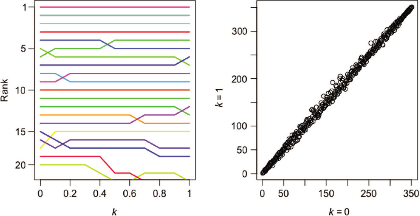
Left: Rankings for 20 teams as k increases from 0 to 1. Right: Scatter plot of k = 0 ranking versus k = 1 ranking for all 351 NCAA D-1 teams.
We also include a sample of the rankings for the 2016-2017 NCAA basketball season according to each of the family of rankings in (40), again with p running from 0 to 1 in steps of 0.10. In keeping with the results of Chartier et al. (2011), one again sees that the most dramatic changes occur as one moves from p = 0 (no rank-flow from losses) to positive values of p (flow from losses turned on but weighted by p).
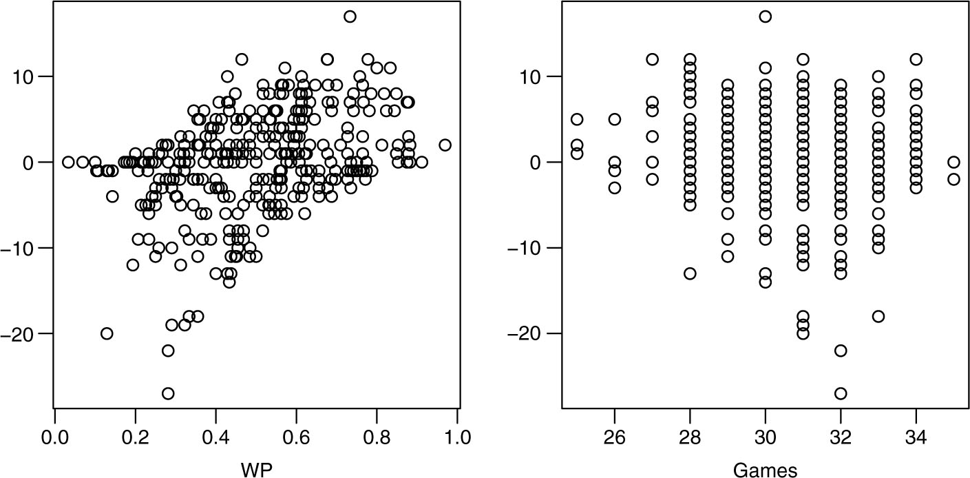
Left: Scatter plot of rank-difference (k = 0 rank minus k = 1 rank) versus team winning percentage (WP) for all 351 teams. Right: Scatter plot of rank-difference versus games played.
It is interesting to note that Gonzaga is ranked first by the Markov method. The Zags were 37–1 on the season and lost in the National Championship game (to North Carolina). Because Gonzaga plays nearly half their games in the mid-tier West Coast Conference, they suffer in ranking methodologies where strength of schedule becomes more important (larger p), and end up ranked below teams like Villanova, Kansas, Arizona, Duke, North Carolina, and Kentucky, all of which play in elite conferences. We also include BYU, who provided the Zags with their only regular season loss, in the Table 1. Not surprisingly BYU fairs considerably better in rankings that weigh wins more than losses (smaller p). BYU is technically a tournament worthy team (top 64) for p < 0.40, but not for any larger value of p.
The last two rows of the table are the teams with the greatest difference in ranking (negative and positive) between p = 0 and p = 1. Indiana State, for example, had an early season upset win against sixteenth ranked Butler that serves them well in the Markov method. That win, however, loses its influence as the right-hand-side infusion vector increases the importance of their 10–20 record (against D1 opponents) on the season. By contrast, Liberty’s ranking improves as their 18–14 (against D1 opponents) record gets more weight despite lacking any signature wins on the season. Neither team played a particularly strong schedule.
6 Effect of virtual games
We briefly explore the effect of adding virtual games via the choice of k in (35).
Figure 3 (left panel) shows the effect of varying k on the rankings of the top twenty teams (as determined with k = 0) in the 16–17 D-1 college basketball season. The right panel shows a scatter plot of each team’s rank using k = 0 and k = 1 for each of the 351 NCAA D-1 teams. All rating vectors have an average value of 0.50. While the rankings are clearly similar, there is a nontrivial effect due to the addition of the virtual games.
Figure 4 gives scatter plots for both the win percentage, and the number of games, respectively, versus the difference in rankings with k = 0 and k = 1, again for each of the 351 D-1 teams. The correlation between difference in rank and wins is r = 0.39, significant at the 0.001 level, while the correlation between difference in rank and games played is r = −0.13, significant only at the 0.05 level, and not below. The intuition here is that the introduction of virtual games in the original Colley method has the effect of a slight watering down of the importance of team record. By choosing k = 0, we effectively increase the importance of win-loss record as indicated by the stronger correlation with wins and positive rank difference in the left panel of Figure 4.
7 Validation
In this section we consider the values of the parameters k in (35) and p in (40) using ten-fold cross validation. We take data from the last 33 NCAA DI college basketball seasons (1985–2017), and in each case, divide the season into ten approximately equal sized sets of games. We hold out one fold as a test set, and train the team rankings with game results from the remaining nine folds. Once rankings are obtained, we create predictions for the games in the test set. Creating game predictions from ratings and rankings is itself a broad subject of considerable interest, but for our purposes we use the simplest possible method and predict the higher ranked team regardless of any other information like home or away status. This process is then repeated so that each of the folds is used as the test set once. Test set prediction accuracy for a season is recorded as the average of the prediction accuracies on each of the ten test sets.
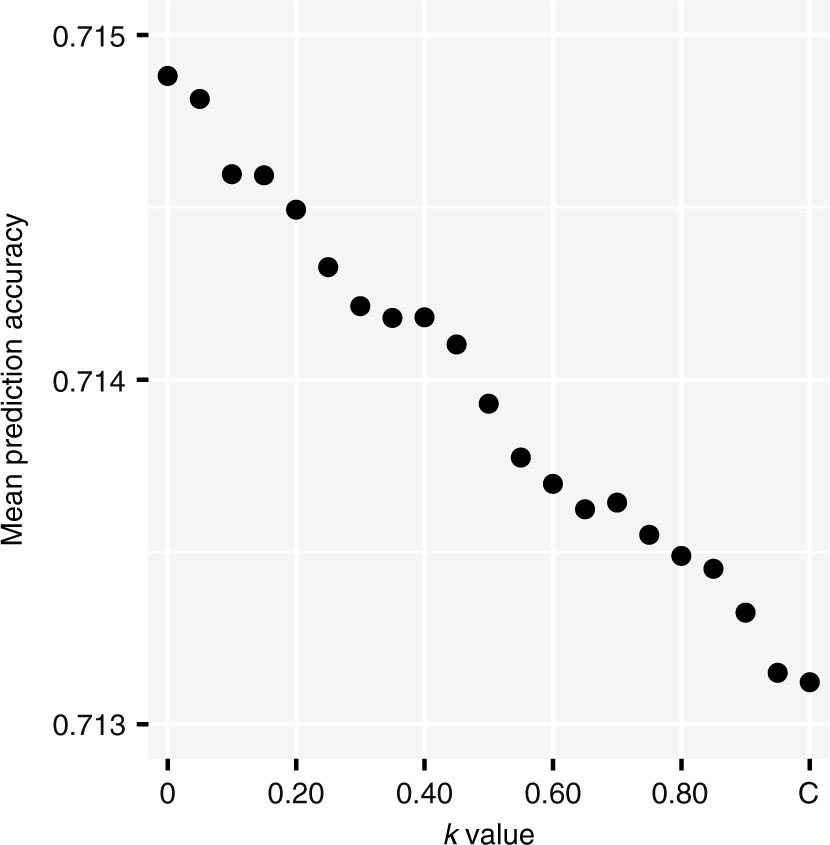
Mean prediction accuracy for values of k. Each point is the mean of the test set prediction accuracy over the last 33 seasons of NCAA DI college basketball. The original Colley method (k = 1) is labeled C.
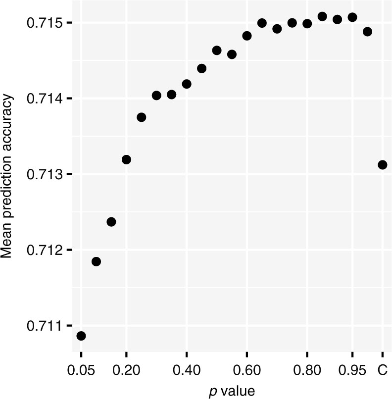
Mean prediction accuracy for values of p. Each point is the mean test prediction accuracy over the last 33 seasons of NCAA DI college basketball. The original Colley method is labeled C.
Figure 5 shows the mean prediction accuracy for each value of k between k = 0 (m-Colley), and the traditional Colley method with k = 1. Each point represents the average of the test set prediction accuracies over the past 33 seasons of NCAA Division I basketball. While the values are certainly similar, there is a clear pattern of decreasing accuracy with larger values of k. Along with the diffusion intuition discussed above, and the results of Section 6, this provides compelling evidence for k = 0 as a natural choice in (35).
Moving to the choice of p, we employ the same cross validation strategy, with results shown in Figure 6. The mean prediction accuracy increases steadily with increasing p, with a maximum value at p = 0.85. The prediction accuracy, however, levels out around p = 0.65 and it is difficult to make a strong case for any one particular value of p between p = 0.65 and p = 1. Notably, however, the traditional Colley method is not competitive with most of the ranking methods given by (40). In 29 of the 33 seasons, the maximum value of the prediction accuracy occurs for a value of p other than 0 or 1.
8 Conclusion
Equation (31) defines a one parameter family of rankings that interpolates between the Markov method [(27) with p = 0] and the (modified) methods of Colley and Massey [(31) with p = 1]. The ratings have a natural interpretation in the context of a diffusion process on a graph. The process is determined by specifying the rank-flow from one team to another in terms of head-to-head wins, weighted by head-to-head losses, and a rank-infusion vector determined by the team’s overall record. This interpretation allows us to realize similarities (and differences) between the methods of Massey, Markov, and Colley, as particular choices of parameters and normalizations made by each method in the in the context of this unifying diffusion paradigm.
The intuition of the diffusion process helps contextualize these choices: if one desires head-to-head results to be relevant in a team’s ranking (beyond their winning percentage), then choose p < 1. If one prefers to emphasize record and strength of schedule, choose p = 1. If the Markov method’s instability seems too extreme to define a reasonable ranking system, take p > 0. On the other hand, if one uses the axiomatic considerations in González-Díaz et al. (2014) that were mentioned earlier, then the choice is simpler. For instance, requiring that the rankings reverse when game results are reversed (the so-called inversion axiom), it is straightforward to show that the axiom is satisfied if and only if p = 1.
We also explore a quantitative validation of the parameter p based on prediction accuracy using ten-fold cross validation in Section 7. The results are interesting, but not conclusive, and suggest several avenues for future work. It would be interesting to consider other validation criteria to see if there is a perspective which suggests an optimal value of p, and whether that p is less than 1. Further, it seems plausible that different sports (or even leagues) might have different optimal p values for their rankings. We used data from NCAA DI college basketball here, but it would be interesting to consider data from other sports with readily available data sets like the NFL, NHL, NBA etc.
We also show that Colley’s method can be generalized to a family of Colley-like ranking methods via Equation (35). Moreover, we give strong evidence that the optimal member of the family is not the traditional Colley method, but rather the diffusion ranker
There are several other directions for future work. First, the diffusion rankings use a particular infusion vector although other choices, like Massey’s original idea of cumulative point difference, are possible and should be studied.
Next, the diffusion paradigm gives an interpretation of the ranking problem in terms of network dynamics, and makes use of a graph Laplacian in the process. Other work has also found interesting network interpretations of ranking problems, notably Csató (2015). Here too, the graph Laplacian is front-and-center, and facilitates an iterative calculation of the least-squares ranking method (called Massey’s method here) using rankings of neighbors along paths of increasing length in the network. Further exploration of the connections between these methods is in order.
Finally, one can consider variations on the Markov method using different coefficient matrices, with one such example in Kvam and Sokol (2006). It would be interesting to interpret these approaches in the context of the diffusion interpretation.
References
Brin, S. and L. Page. 1998. “The Anatomy of a Large-Scale Hypertextual Web Search Engine.” Computer Networks and ISDN Systems. 30(1–7):107–117.10.1016/S0169-7552(98)00110-XSearch in Google Scholar
Callaghan, T., P. J. Mucha, and M. A. Porter. 2007. “Random Walker Ranking for NCAA Division IA Football.” American Mathematical Monthly 114(9):761–777.10.1080/00029890.2007.11920469Search in Google Scholar
Chartier, T. P., E. Kreutzer, A. N. Langville, and K. E. Pedings. 2011. “Sensitivity and Stability of Ranking Vectors.” SIAM Journal on Scientific Computing 33(3):1077–1102.10.1137/090772745Search in Google Scholar
Colley, W. N. 2002. Colley’s Bias Free College Football Ranking Method: The Colley Matrix Explained. Princeton: Princeton University.Search in Google Scholar
Csató, L. 2015. “A Graph Interpretation of the Least Squares Ranking Method.” Social Choice and Welfare 44(1):51–69.10.1007/s00355-014-0820-0Search in Google Scholar
Cvetkovic, D. M., M. Doob, and H. Sachs. 1980. Spectra of Graphs: Theory and Application. Berlin, New York: Deutscher Verlag der Wissenschaften, Academic Press.Search in Google Scholar
Doyle, P. G. and J. L. Snell. 2000. “Random Walks and Electric Networks.” Free Software Foundation. Accessed June 1, 2018 (https://math.dartmouth.edu/∼doyle/docs/walks/walks.pdf).10.5948/UPO9781614440222Search in Google Scholar
Glickman, M. E. and H. S. Stern. 2017. “Estimating Team Strength in the NFL.” Pp. 113–136 in Handbook of Statistical Methods and Analyses in Sports, chapter 5, edited by J. Albert, M. E. Glickman, T. B. Swarz, and R. H. Koning. Boca Raton, FL: CRC Press.10.1201/9781315166070Search in Google Scholar
González-Díaz, J., R. Hendrickx, and E. Lohmann. 2014. “Paired Comparisons Analysis: An Axiomatic Approach to Ranking Methods.” Social Choice and Welfare 42(1):139–169.10.1007/s00355-013-0726-2Search in Google Scholar
Horst, P. 1932. “A Method for Determining the Absolute Affective Value of a Series of Stimulus Situations.” Journal of Educational Psychology 23(6):418.10.1037/h0070134Search in Google Scholar
Kendall, M. G. and B. B. Smith. 1940. “On the Method of Paired Comparisons.” Biometrika 31(3/4):324–345.10.1093/biomet/31.3-4.324Search in Google Scholar
Kvam, P. and J. S. Sokol. 2006. “A Logistic Regression/Markov Chain Model for NCAA Basketball.” Naval Research Logistics (NRL) 53(8):788–803.10.1002/nav.20170Search in Google Scholar
Langville, A. N. and C. D. Meyer. 2012. Who’s #1?: The Science of Rating and Ranking. Princeton, NJ: Princeton University Press.10.1515/9781400841677Search in Google Scholar
Massey, K. 1997. “Statistical Models Applied to the Rating of Sports Teams.” Bluefield College. Accessed June 1, 2018 (https://www.masseyratings.com/theory/massey97.pdf).Search in Google Scholar
Mattingly, R. and A. Murphy. 2010. “A Markov Method for Ranking College Football Conferences.” Accessed June 1, 2018 (http://www.mathaware.org/mam/2010/essays/Mattingly.pdf).Search in Google Scholar
Meyer, C. D. 2000. Matrix Analysis and Applied Linear Algebra, volume 2. Philadelphia: Siam.10.1137/1.9780898719512Search in Google Scholar
Mosteller, F. 1951. “Remarks on the Method of Paired Comparisons: I. The Least Squares Solution Assuming Equal Standard Deviations and Equal Correlations.” Psychometrika 16(1):3–9.10.1007/978-0-387-44956-2_8Search in Google Scholar
Newman, M. 2010. Networks: An Introduction. Oxford: OUP.10.1093/acprof:oso/9780199206650.001.0001Search in Google Scholar
Stefani, R. 2011. “The Methodology of Officially Recognized International Sports Rating Systems.” Journal of Quantitative Analysis in Sports 7(4). doi:10.2202/1559-0410.1347.10.2202/1559-0410.1347Search in Google Scholar
Vaziri, B., S. Dabadghao, Y. Yih, and T. L. Morin. 2018. “Properties of Sports Ranking Methods.” Journal of the Operational Research Society 69(5):776–787.10.1057/s41274-017-0266-8Search in Google Scholar
Von Hilgers, P. and A. N. Langville. 2006. “The Five Greatest Applications of Markov Chains.” In Proceedings of the Markov Anniversary Meeting. Boston, MA: Boston Press.Search in Google Scholar
©2018 Walter de Gruyter GmbH, Berlin/Boston
Articles in the same Issue
- Frontmatter
- A network diffusion ranking family that includes the methods of Markov, Massey, and Colley
- Quantifying the probability of a shot in women’s collegiate soccer through absorbing Markov chains
- Modelling the dynamic pattern of surface area in basketball and its effects on team performance
- A Bayesian regression approach to handicapping tennis players based on a rating system
- Bayesian hierarchical models for predicting individual performance in soccer