Stability Analysis of Double Diffusive Convection in Local Thermal Non-equilibrium Porous Medium with Internal Heat Source and Reaction Effects

Najat J. Noon; Shatha A. Haddad

doi:10.1515/jnet-2022-0047

Article Publicly Available

Stability Analysis of Double Diffusive Convection in Local Thermal Non-equilibrium Porous Medium with Internal Heat Source and Reaction Effects

Najat J. Noon and Shatha A. Haddad

Published/Copyright: September 20, 2022

Published by

Become an author with De Gruyter Brill

Submit Manuscript Author Information

From the journal Journal of Non-Equilibrium Thermodynamics Volume 48 Issue 1

Abstract

The internal heat source and reaction effects on the onset of thermosolutal convection in a local thermal non-equilibrium porous medium are examined, where the temperature of the fluid and the solid skeleton may differ. The linear instability and nonlinear stability theories of Darcy–Brinkman type with fixed boundary condition are carried out where the layer is heated and salted from below. The D 2 Chebyshev tau technique is used to calculate the associated system of equations subject to the boundary conditions for both theories. Three different types of internal heat source function are considered, the first type increases across the layer, while the second decreases, and the third type heats and cools in a nonuniform way. The effect of different parameters on the Rayleigh number is depicted graphically. Moreover, the results detect that utilizing the internal heat source, reaction, and non-equilibrium have pronounced effects in determining the convection stability and instability thresholds.

Keywords: stability analysis; double diffusive convection; internal heat source effect; reaction effect; Darcy–Brinkman model; local thermal non-equilibrium; porous media

1 Introduction

Thermal convection in a saturated porous material is a subject of increasing interest. Recent research has given special interest on thermal convection in a porous medium where the fluid temperature T f may differ from the solid skeleton temperature T s . Local thermal non-equilibrium is the term used to describe the situation where the two temperatures may differ. There are many practical applications of this subject area, which may be the main factor contributing to the rising interest in local thermal non-equilibrium flows in porous medium; see, e. g., Straughan [1], Celli et al. [2], Choudhary et al. [3], Straughan [4], [5], Celli et al. [6], Mankhi and Haddad [7], Capone and Gianfrani [8]. Another interesting study on the stability theory that considers the convection in fluid-saturated porous medium induced by internal heating has been given by Nouri-Borujerdi et al. [9], [10], Kuznetsov and Nield [11], Mahajan and Nandal [12], [13], Siddabasappa and Sakshath [14]. Mahajan and Nandal [13] analyzed the onset of convection with local thermal non-equilibrium porous media for the Darcy–Brinkman model. Four types of internal heat-generating function were considered. The effect of various parameters on the onset of convection was discussed and illustrated numerically by using the Chebyshev pseudospectral method. Siddabasappa and Sakshath [14] investigated the stability analysis of Darcy–Brinkman convection with local thermal non-equilibrium porous medium in the presence of internal heat source in two ways, in a liquid phase and in a solid phase; they discussed the effect of different coefficients on the onset of convection and depicted them graphically.

The thermosolutal (double-diffusive) convection in porous media is a topic of increasing attention due to its prevalence in a wide range of real situations. It has attracted many researchers; see, e. g., Sharma et al. [15], Pritchard and Richardson [16], Wang and Tan [17], Liu and Umavathi [18], Mahajan and Tripathi [19], and Noon and Haddad [20]. For the case of a local thermal non-equilibrium flow in a porous medium, see, e. g., Malashetty et al. [21], Malashetty and Heera [22], Chen et al. [23], Malashetty et al. [24], Nield et al. [25], Kuznetsov et al. [26], Altawallbeh et al. [27], Kumar et al. [28], and Hemanth Kumar et al. [29]. Chen et al. [23] studied the onset of double-diffusive convection in a porous medium with local thermal non-equilibrium and reaction effect for Darcy model; the effect of various coefficients on the onset of convection was discussed numerically. Kuznetsov et al. [26] analyzed the onset of thermosolutal convection in a local thermal non-equilibrium porous medium for Darcy model composed of two horizontal layers that were internally heated; the effects of parameter variations were discussed numerically using Galerkin method.

In this paper, the onset of thermosolutal convection with the internal heat source and reaction effects in a fluid-saturated porous media under the condition of a local thermal non-equilibrium for the Darcy–Brinkman model is studied with a fixed boundary condition where the layer is heated and salted from below. Three different types of internal heat source function are considered, the first type increases across the layer, while the second decreases, and the third type heats and cools in a nonuniform way. Our goal is here to investigate the effects of the internal heat source, reaction, and local thermal non-equilibrium on the stability of the system. The D 2 Chebyshev tau method is used to solve the eigenvalue problem and analyze the linear and nonlinear stability thresholds.

To this end, the governing equations and appropriate steady-state solutions are presented in Section 2. In Sections 3 and 4, the linear instability and the nonlinear stability theories are presented. The numerical method is generated by using the D 2 Chebyshev tau technique for fixed surface boundaries in Section 5. The effects of the internal heat source, the reaction terms, and local thermal non-equilibrium on the Rayleigh number are graphically represented in Section 6. In the final Section 7, the conclusion is discussed.

2 Governing equations

Let us consider a layer of fluid saturated a porous material that is bounded by two horizontal planes and a vertical axis z, { ( x , y ) ∈ R 2 } × { z ∈ ( 0 , d ) } . The upper plane z = d is maintained at a constant temperature T U and salt concentration C U , while the lower plane z = 0 is maintained at constant temperature T L and salt concentration C L . The Darcy–Brinkman equation in double diffusive convection is considered with an internal heat source, allowing gravity g to be determined by the vertical coordinate z as shown in Figure 1. The governing equations can be represented as follows:

(1) p , i = − μ K v i − ρ 0 [ 1 − α T ( T f − T L ) + α C ( C − C L ) ] g k i + λ Δ v i , v i , i = 0 , ϕ ˆ ( ρ c ) f T , t f + ( ρ c ) f v i T , i f = ϕ ˆ k f Δ T f + h ˆ ( T s − T f ) + ϕ ˆ Q f ( z ) , ( 1 − ϕ ˆ ) ( ρ c ) s T , t s = ( 1 − ϕ ˆ ) k s Δ T s + h ˆ ( T f − T s ) + ( 1 − ϕ ˆ ) Q s ( z ) , ϕ ˆ C , t + v i C , i = ϕ ˆ k C Δ C + k ˆ [ C e q ( T f ) − C ] ,

where v i , p, T, C, C e q are the velocity, pressure, temperature, salt concentration, and equilibrium concentration of solute at a given temperature, respectively, the subscript f and s refer to the fluid and solid phase properties, respectively, μ, λ are viscosities, h ˆ is the inter phase heat transfer coefficient, g, ρ 0 , α T , α C , k, k C , k ˆ , Q ( z ) , and ϕ ˆ are gravity, density of fluid at the bottom, thermal expansion coefficient, solute expansion coefficient, the thermal conductivity, the molecular diffusivity of the solute through the fluid, the lumped effective reaction rate, the internal heat source, and the matrix porosity, respectively. The equilibrium solute concentration is assumed as a linear function of temperature as in Pritchard and Richardson [16] such that C e q ( T f ) = f 1 ( T f − T L ) + f 0 , where f 1 and f 0 are constants. The boundary conditions are

(2) v i = 0 , on z = 0 , d , T f = T s = T L , C = C L , on z = 0 , T f = T s = T U , C = C U , on z = d .

Here T L > T U and C L > C U for the heated and salted below layer case. Three types of heat-generating function are considered in this study: linearly increasing, decreasing, and nonuniform, see Straughan [30]:

Case A: Q ( z ) = Q 0 ( 1 2 + 1 d z ) , Case B: Q ( z ) = Q 0 ( 2 + 3 2 d 2 z 2 − 3 d z ) , Case C: Q ( z ) = Q 0 ( 1 + sin 2 π d z + sin 4 π d z ) ,

where Q 0 > 0 . In the steady state solution, we look for

(3) v ¯ i = 0 , T ¯ f = T ¯ s = T ¯ ( z ) , C ¯ = C ¯ ( z ) .

From eq. (1)_3–4, using cases A–C, and eq. (3), we get

k f Δ T ¯ f = − Q f ( z ) , k s Δ T ¯ s = − Q s ( z )

and, by using eq. (2), then

(4) v ¯ i = 0 , T ¯ f = − Q 0 k f [ 1 4 z 2 + 1 6 d z 3 − 5 d 12 z ] − β T z + T L , − Q 0 k f [ z 2 + 1 8 d 2 z 4 − 1 2 d z 3 − 5 d 8 z ] − β T z + T L , − Q 0 k f [ 1 2 z 2 − d 2 4 π 2 sin 2 π d z − d 2 16 π 2 sin 4 π d z − d 2 z ] − β T z + T L , T ¯ s = − Q 0 k s [ 1 4 z 2 + 1 6 d z 3 − 5 d 12 z ] − β T z + T L , − Q 0 k s [ z 2 + 1 8 d 2 z 4 − 1 2 d z 3 − 5 d 8 z ] − β T z + T L , − Q 0 k s [ 1 2 z 2 − d 2 4 π 2 sin 2 π d z − d 2 16 π 2 sin 4 π d z − d 2 z ] − β T z + T L ,

where β T = T L − T U d . Also, ϕ ˆ k C Δ C ¯ + k ˆ ( C e q ( T ¯ f ) − C ¯ ) = 0 . As presented by Pritchard and Richardson [16], assume that C ¯ ( z ) = C e q ( T ¯ f ( z ) ) . Hence,

ϕ ˆ k C Δ C ¯ = 0 ,

which gives

C ( z ) ¯ = a T ¯ f ( z ) + b ,

where a and b are constants of integration. Now, using eq. (2) gives

(5) C ¯ = − β C Q 0 β T k f [ 1 4 z 2 + 1 6 d z 3 − 5 d 12 z ] − β C z + C L , − β C Q 0 β T k f [ z 2 + 1 8 d 2 z 4 − 1 2 d z 3 − 5 d 8 z ] − β C z + C L , − β C Q 0 β T k f [ 1 2 z 2 − d 2 4 π 2 sin 2 π d z − d 2 16 π 2 sin 4 π d z − d 2 z ] − β C z + C L ,

where β C = C L − C U d . To analyze the stability of the solutions in Eqs. (4)–(5), we define perturbations ( u i , π , θ f , θ s , ϕ ) such that

(6) v i = v ¯ i + u i , p = p ¯ + π , T f = T ¯ f + θ f , T s = T ¯ s + θ s , C = C ¯ + ϕ .

Substituting eq. (6) into eq. (1), we obtain the equations governing ( u i , π , θ , ϕ ) as

(7) π , i = − μ K u i + ρ 0 α T g k i θ f − ρ 0 α C g k i ϕ + λ Δ u i , u i , i = 0 , ϕ ˆ ( ρ c ) f θ , t f + ( ρ c ) f u i θ , i f = − ( ρ c ) f d T ¯ f d z w + ϕ ˆ k f Δ θ f + h ˆ ( θ s − θ f ) , ( 1 − ϕ ˆ ) ( ρ c ) s θ , t s = ( 1 − ϕ ˆ ) k s Δ θ s + h ˆ ( θ f − θ s ) , ϕ ˆ ϕ , t + u i ϕ , i = − d C ¯ d z w + ϕ ˆ k C Δ ϕ + k ˆ f 1 θ f − k ˆ ϕ ,

where u = ( u , v , w ) . Using nondimensionalization, we use the length scale d, time scale τ = ( ρ c ) f d 2 k f , velocity scale U = ϕ ˆ k f ( ρ c ) f d , pressure scale P = ϕ ˆ k f μ ( ρ c ) f K , the temperature T ♯ = Q 0 d 2 k f R , and the concentration scale C ♯ = β C Q 0 d 2 β T k f R s . Here, ϵ = L e ( ρ c ) f , L e = k f k C is the Lewis number, and γ ˜ = λ K d 2 μ is the Brinkman coefficient. The thermal Rayleigh and solutal Rayleigh numbers are defined as follows:

R 2 = d 3 K Q 0 α T ρ 0 g ϕ ˆ k f μ κ , R s 2 = β C d 3 K Q 0 α C ρ 0 g β T ϕ ˆ k f μ κ .

After substituting the nondimensionalization scalings into eq. (7), we have

(8) π , i = − u i + R k i θ f − R s k i ϕ + γ ˜ Δ u i , u i , i = 0 , θ , t f + u i θ , i f = R N ( z ) w + Δ θ f + H ˆ ( θ s − θ f ) , A ˆ θ , t s = Δ θ s + λ ˆ H ˆ ( θ f − θ s ) , ϵ ϕ , t + ϵ u i ϕ , i = ϵ R s N ( z ) w + Δ ϕ + h θ f − η ϕ ,

where

N ( z ) = 1 2 z 2 + 1 2 z − 5 12 + ζ , 1 2 z 3 − 3 2 z 2 + 2 z − 5 8 + ζ , z − 1 2 π cos 2 π z − 1 4 π cos 4 π z − 1 2 + ζ .

Here, the heat parameter is ζ = β T k f Q 0 d . Furthermore, the interphase heat transfer parameter is H ˆ = h ˆ d 2 ϕ ˆ k f , A ˆ = k f ( ρ c ) s k s ( ρ c ) f is the diffusivity ratio, the porosity modified conductivity ratio is λ ˆ = ϕ ˆ k f ( 1 − ϕ ˆ ) k s , while h and η are the reaction terms given by

h = k ˆ f 1 d 2 T ♯ ϕ ˆ k C C ♯ , η = k ˆ d 2 ϕ ˆ k C .

Equation (8) hold in the domain { ( x , y ) ∈ R 2 } × { z ∈ ( 0 , 1 ) } × { t > 0 } . The boundary conditions become

u i = θ = ϕ = 0 on z = 0 , 1 .

Figure 1

Physical configuration of the double-diffusive convection.

3 Linear instability theory

To perform the linear instability analysis, we first remove the nonlinear terms of Eqs. (8)_3–5and then remove the π term by taking the third component of the double curl of eq. (8)₁. We seek for solutions of the form

w ( x , t ) = w ( x ) e σ t , θ f ( x , t ) = θ f ( x ) e σ t , θ s ( x , t ) = θ s ( x ) e σ t , ϕ ( x , t ) = ϕ ( x ) e σ t ,

where σ is the time-dependent growth rate. Thus, the linearized equations arising from eq. (8) are

(9) Δ w − R Δ ∗ θ f + R s Δ ∗ ϕ − γ ˜ Δ 2 w = 0 , σ θ f = R N ( z ) w + Δ θ f + H ˆ ( θ s − θ f ) , A ˆ σ θ s = Δ θ s + λ ˆ H ˆ ( θ f − θ s ) , ϵ σ ϕ = ϵ R s N ( z ) w + Δ ϕ + h θ f − η ϕ ,

where Δ ∗ = ∂ 2 ∂ x 2 + ∂ 2 ∂ y 2 is the horizontal Laplacian operator. To analyze equations in eq. (9), we use standard methods, cf. Chandrasekhar [31]. Then we assume the normal mode with the representations for w, θ f , θ s , and ϕ in the form of

w = W ( z ) f ( x , y ) , θ f = Θ f ( z ) f ( x , y ) , θ s = Θ s ( z ) f ( x , y ) , ϕ = Φ ( z ) f ( x , y ) ,

where f is the horizontal plane form which satisfies Δ ∗ f = − a 2 f , D = d d z , a is a wave number, and Δ = D 2 − a 2 . The system in eq. (9) may be written in the form

(10) ( D 2 − a 2 ) W − γ ˜ ( D 2 − a 2 ) 2 W + a 2 R Θ f − a 2 R s Φ = 0 , σ Θ f = R N ( z ) W + ( D 2 − a 2 ) Θ f + H ˆ ( Θ s − Θ f ) , A ˆ σ Θ s = ( D 2 − a 2 ) Θ s + λ ˆ H ˆ ( Θ f − Θ s ) , ϵ σ Φ = ϵ R s N ( z ) W + h Θ f + ( D 2 − a 2 ) Φ − η Φ .

Equation (10) represents an eigenvalue problem for the eigenvalue σ to be found subject to the boundary conditions

(11) W = D W = Θ = Φ = 0 on z = 0 , 1 .

We determine the critical Rayleigh number by

R a = min a 2 R 2 ( a 2 ) ,

where for all R 2 > R a the system is unstable.

4 Nonlinear stability theory

In this section, the nonlinear energy stability analysis is provided to give a threshold in which the system is stable. To this end, let V be a period cell for the disturbance solution defined by Γ × { z ∈ ( 0 , d ) } , where Γ denotes the cell shape in the horizontal plane ( x , y ) and let ‖·‖ and ⟨·⟩ be the norm and inner product on L 2 ( V ) . Then, by multiplying eqs. (8)_1,3–5 by w, θ f , θ s , and ϕ, respectively, and integrating each over V, we find

(12) − ‖ u ‖ 2 + R ⟨ θ f , w ⟩ − R s ⟨ ϕ , w ⟩ − γ ˜ ‖ ∇ u ‖ 2 = 0 , 1 2 d d t ‖ θ f ‖ 2 = R N ( z ) ⟨ w , θ f ⟩ − ‖ ∇ θ f ‖ 2 + H ˆ ⟨ θ s , θ f ⟩ − H ˆ ‖ θ f ‖ 2 , A ˆ 2 d d t ‖ θ s ‖ 2 = − ‖ ∇ θ s ‖ 2 + λ ˆ H ˆ ⟨ θ f , θ s ⟩ − λ ˆ H ˆ ‖ θ s ‖ 2 , ϵ 2 d d t ‖ ϕ ‖ 2 = ϵ R s N ( z ) ⟨ w , ϕ ⟩ − ‖ ∇ ϕ ‖ 2 + h ⟨ θ f , ϕ ⟩ − η ‖ ϕ ‖ 2 .

Then we form the combination of the equations in eq. (12) as λ 1 (12)₁ + (12)₂ + (12)₃ + λ 2 (12)₄, where λ 1 and λ 2 are positive numbers to be chosen. This leads to the energy equation

(13) d E d t = I − D = − D ( 1 − I D ) ,

where

(14) E = 1 2 ‖ θ f ‖ 2 + A ˆ 2 ‖ θ s ‖ 2 + λ 2 ϵ 2 ‖ ϕ ‖ 2 , I = R ( λ 1 + N ( z ) ) ⟨ θ f , w ⟩ + R s ( ϵ λ 2 N ( z ) − λ 1 ) ⟨ ϕ , w ⟩ + H ˆ ( 1 + λ ˆ ) ⟨ θ f , θ s ⟩ + λ 2 h ⟨ θ f , ϕ ⟩ , D = λ 1 ‖ u ‖ 2 + λ 1 γ ˜ ‖ ∇ u ‖ 2 + ‖ ∇ θ f ‖ 2 + H ˆ ‖ θ f ‖ 2 + ‖ ∇ θ s ‖ 2 + λ ˆ H ˆ ‖ θ s ‖ 2 + λ 2 ‖ ∇ ϕ ‖ 2 + λ 2 η ‖ ϕ ‖ 2 .

Then

(15) d E d t ≤ − D ( 1 − max H I D ) = − D ( 1 − 1 R E ) ,

where H is the space of admissible solutions and

(16) 1 R E = max H I D .

The nonlinear stability follows when R E > 1 , which implies that ( 1 − 1 R E ) > 0 . From eq. (14)₃ and by using Poincaré’s inequality, one may obtain

(17) D = λ 1 ‖ u ‖ 2 + λ 1 γ ˜ ‖ ∇ u ‖ 2 + ‖ ∇ θ f ‖ 2 + H ˆ ‖ θ f ‖ 2 + ‖ ∇ θ s ‖ 2 + λ ˆ H ˆ ‖ θ s ‖ 2 + λ 2 ‖ ∇ ϕ ‖ 2 + λ 2 η ‖ ϕ ‖ 2 ≥ ( H ˆ + π 2 ) ‖ θ f ‖ 2 + ( λ ˆ H ˆ + π 2 ) ‖ θ s ‖ 2 + λ 2 π 2 ‖ ϕ ‖ 2 = ( H ˆ + π 2 ) ‖ θ f ‖ 2 + A ˆ A ˆ ( λ ˆ H ˆ + π 2 ) ‖ θ s ‖ 2 + λ 2 ϵ ϵ π 2 ‖ ϕ ‖ 2 ≥ 2 k ( ‖ θ f ‖ 2 + A ˆ ‖ θ s ‖ 2 + λ 2 ϵ ‖ ϕ ‖ 2 2 ) = 2 k E ,

where k = min { H ˆ + π 2 , λ ˆ H ˆ + π 2 A ˆ , π 2 ϵ } . Then from eq. (15) one may derive the inequality

d E d t ≤ − 2 k b E ,

where b = 1 − 1 R E .

This may be integrated to see that

(18) E ( t ) ≤ E ( 0 ) e − 2 k b t ,

where E ( 0 ) is constant, and hence we see that E ( t ) ⟶ 0 as t ⟶ ∞ . Therefore, by the definition of E, one proves that ‖ θ f ‖ ⟶ 0 , ‖ θ s ‖ ⟶ 0 , and ‖ ϕ ‖ ⟶ 0 as t ⟶ ∞ .

To obtain the decay of u, by using the Poincaré and arithmetic–geometric mean inequalities in eq. (12)₁, we can then deduce that

(19) ( 1 + γ ˜ π 2 ) ‖ u ‖ 2 ≤ R 2 ν 1 ‖ θ f ‖ 2 + R ν 1 2 ‖ w ‖ 2 + R s 2 ν 2 ‖ ϕ ‖ 2 + R s ν 2 2 ‖ w ‖ 2 ≤ ( R ν 1 2 + R s ν 2 2 ) ‖ u ‖ 2 + R 2 ν 1 ‖ θ f ‖ 2 + R s 2 ν 2 ‖ ϕ ‖ 2 ,

where ν 1 and ν 2 are constants to be chosen such that R ν 1 + R s ν 2 = 1 , which gives ν 1 = 1 R and ν 2 = 1 R s , so to that inequality (19) will be

‖ u ‖ 2 ≤ R 2 2 γ ˜ π 2 ‖ θ f ‖ 2 + R s 2 2 γ ˜ π 2 ‖ ϕ ‖ 2 .

Therefore we see that ‖ u ‖ ⟶ 0 as t ⟶ ∞ , so we have shown the decay of u, θ f , θ s , and ϕ.

The nonlinear stability threshold is thus given by the solution of the variational problem in eq. (16). The Euler–Lagrange equations for the latter are

(20) R ( λ 1 + N ( z ) ) θ f k i + R s ( ϵ λ 2 N ( z ) − λ 1 ) ϕ k i − 2 λ 1 u i + 2 λ 1 γ ˜ Δ u i = ξ , i , R ( λ 1 + N ( z ) ) w + 2 Δ θ f − 2 H ˆ θ f + H ˆ ( 1 + λ ˆ ) θ s + λ 2 h ϕ = 0 , H ˆ ( 1 + λ ˆ ) θ f + 2 Δ θ s − 2 λ ˆ H ˆ θ s = 0 , R s ( ϵ λ 2 N ( z ) − λ 1 ) w + λ 2 h θ f + 2 λ 2 Δ ϕ − 2 λ 2 η ϕ = 0 ,

where ξ is a Lagrange multiplier. By taking the double curl of eq. (20)₁, and introducing the normal mode representation as presented in Sect. 3, eq. (20) becomes

(21) 2 λ 1 ( D 2 − a 2 ) W − 2 λ 1 γ ˜ ( D 2 − a 2 ) 2 W + a 2 R ( λ 1 + N ( z ) ) Θ f + a 2 R s ( ϵ λ 2 N ( z ) − λ 1 ) Φ = 0 , R ( λ 1 + N ( z ) ) W + 2 ( D 2 − a 2 ) Θ f − 2 H ˆ Θ f + H ˆ ( 1 + λ ˆ ) Θ s + λ 2 h Φ = 0 , H ˆ ( 1 + λ ˆ ) Θ f + 2 ( D 2 − a 2 ) Θ s − 2 λ ˆ H ˆ Θ s = 0 , R s ( ϵ λ 2 N ( z ) − λ 1 ) W + λ 2 h Θ f + 2 λ 2 ( D 2 − a 2 ) Φ − 2 λ 2 η Φ = 0 ,

The corresponding boundary conditions are in eq. (11). We can determine the critical Rayleigh number

R a E = max λ 1 , λ 2 min a 2 R 2 ( a 2 , λ 1 , λ 2 ) ,

where for all R 2 < R a E the system is stable.

5 Numerical method

In this section, the bound for the linear instability theory and the energy theory of Eqs. (10) and (21), respectively, corresponding to boundary conditions eq. (11), are solved numerically by using a D 2 Chebyshev tau method, see Dongarra et al. [32]. The numerical results for the heated and salted below layer are reported in detail in Sect. 6. We can write Eqs. (10)₁ and (21)₁ as second-order equations by setting

χ = ( D 2 − a 2 ) W .

To this end, we begin by resetting the domain from (0,1) to (−1,1), selecting z ˆ = 2 z − 1 . Then, we may rewrite Eqs. (10) and (21), respectively, as the follows (omitting the hat):

(22) ( 4 D 2 − a 2 ) W − χ = 0 , χ − γ ˜ ( 4 D 2 − a 2 ) χ + a 2 R Θ f − a 2 R s Φ = 0 , σ Θ f = R N 1 W + ( 4 D 2 − a 2 ) Θ f + H ˆ ( Θ s − Θ f ) , A ˆ σ Θ s = ( 4 D 2 − a 2 ) Θ s + λ ˆ H ˆ ( Θ f − Θ s ) , ϵ σ Φ = ϵ R s N 1 W + h Θ f + ( 4 D 2 − a 2 ) Φ − η Φ .

(23) ( 4 D 2 − a 2 ) W − χ = 0 , λ 1 χ − λ 1 γ ˜ ( 4 D 2 − a 2 ) χ + a 2 R ( λ 1 + N 1 ) 2 Θ f + a 2 R s ( ϵ λ 2 N 1 − λ 1 ) 2 Φ = 0 , R ( λ 1 + N 1 ) 2 W + ( 4 D 2 − a 2 ) Θ f − H ˆ Θ f + H ˆ ( 1 + λ ˆ ) 2 Θ s + λ 2 h 2 Φ = 0 , H ˆ ( 1 + λ ˆ ) 2 Θ f + ( 4 D 2 − a 2 ) Θ s − λ ˆ H ˆ Θ s = 0 , R s ( ϵ λ 2 N 1 − λ 1 ) 2 W + λ 2 h 2 Θ f + λ 2 ( 4 D 2 − a 2 ) Φ − λ 2 η Φ = 0 ,

where N 1 = N ( z + 1 2 ) , z ∈ ( − 1 , 1 ) . Then, the functions W, χ, Θ f , Θ s , and Φ are expanded in terms of Chebyshev polynomials

W ( z ) = ∑ n = 1 M W n T n ( z ) , χ ( z ) = ∑ n = 1 M χ n T n ( z ) , Θ f ( z ) = ∑ n = 1 M Θ n f T n ( z ) , Θ s ( z ) = ∑ n = 1 M Θ n s T n ( z ) , Φ ( z ) = ∑ n = 1 M Φ n T n ( z ) .

Therefore, the D 2 Chebyshev tau method requires solving the matrix system of eq. (22), namely

(24) A X = σ B X ,

where X = ( W 1 , W 2 , … , W M , χ 1 , χ 2 , … , χ M , Θ 1 f , Θ 2 f , … , Θ M f , Θ 1 s , Θ 2 s , … , Θ M s , Φ 1 , Φ 2 , … , Φ M ) and the matrices A and B are given by

A = 4 D 2 − a 2 I − I 0 0 0 0 I − γ ˜ ( 4 D 2 − a 2 I ) a 2 R I 0 − a 2 R s I R N 1 I 0 4 D 2 − ( a 2 + H ˆ ) I H ˆ I 0 0 0 λ ˆ H ˆ I 4 D 2 − ( a 2 + λ ˆ H ˆ ) I 0 ϵ R s N 1 I 0 h I 0 4 D 2 − ( a 2 + η ) I , B = 0 0 0 0 0 0 0 0 0 0 0 0 I 0 0 0 0 0 A ˆ I 0 0 0 0 0 ϵ I .

And for eq. (23), the matrix system is

(25) C X = R F X ,

where the matrices C and F are given by

C = 4 D 2 − a 2 I − I 0 0 0 0 λ 1 ( I − γ ˜ ( 4 D 2 − a 2 I ) ) 0 0 a 2 R s ( ϵ λ 2 N 1 − λ 1 ) 2 I 0 0 4 D 2 − ( a 2 + H ˆ ) I ( 1 + λ ˆ ) 2 H ˆ I λ 2 h 2 I 0 0 ( 1 + λ ˆ ) 2 H ˆ I 4 D 2 − ( a 2 + λ ˆ H ˆ ) I 0 R s ( ϵ λ 2 N 1 − λ 1 ) 2 I 0 λ 2 h 2 I 0 λ 2 ( 4 D 2 − ( a 2 + η ) I ) , F = 0 0 0 0 0 0 0 − a 2 ( λ 1 + N 1 ) 2 I 0 0 − ( λ 1 + N 1 ) 2 I 0 0 0 0 0 0 0 0 0 0 0 0 0 0 .

Subject to the boundary conditions in eq. (11), where the relations T n ( ± 1 ) = ( ± 1 ) n and T n ′ ( ± 1 ) = ( ± 1 ) n − 1 n 2 are used, we get

(26) W ( − 1 ) = ∑ n = 1 M ( − 1 ) n W ( − 1 ) = 0 , W ( 1 ) = ∑ n = 1 M W ( 1 ) = 0 , D W ( − 1 ) = ∑ n = 1 M ( − 1 ) n − 1 n 2 W ( − 1 ) = 0 , D W ( 1 ) = ∑ n = 1 M n 2 W ( 1 ) = 0 , Θ ( − 1 ) = ∑ n = 1 M ( − 1 ) n Θ ( − 1 ) = 0 , Θ ( 1 ) = ∑ n = 1 M Θ ( 1 ) = 0 , Φ ( − 1 ) = ∑ n = 1 M ( − 1 ) n Φ ( − 1 ) = 0 , Φ ( 1 ) = ∑ n = 1 M Φ ( 1 ) = 0 .

The eigenvalues of the generalized eigenvalue problems (24) and (25) are found efficiently by using the Q Z algorithm.

6 Numerical results and discussion

In this section, the internal heat source and the reaction effects on the threshold thermal Rayleigh number are investigated using thermal non-equilibrium Darcy–Brinkman model. The numerical results are obtained by various parameters with respect to three different types of the internal heat source:

Case A: N 1 ( z ) = ( z + 1 ) 2 8 + z + 1 4 − 5 12 + ζ , Case B: N 1 ( z ) = ( z + 1 ) 3 16 − 3 ( z + 1 ) 2 8 + z + 3 8 + ζ , Case C: N 1 ( z ) = z + 1 2 + 1 2 π cos π z − 1 4 π cos 2 π z − 1 2 + ζ ,

and subject to the boundary conditions in eq. (26). The numerical results are discussed for different choices of the reaction rates η, h, interphase heat transfer parameter H ˆ , porosity modified conductivity ratio λ ˆ , heat parameter ζ, and salt Rayleigh number R s 2 . The cases A–C to have encoded the behavior of various physical coefficients to verify their effect on the stability of the system.

For different values of H ˆ with fixed R s 2 = 5 , γ ˜ = 1 , A ˆ = 1 , λ ˆ = 0.5 , and ζ = 0.6 , when η > h , η < h , and η = h , Table 1 shows that the critical Rayleigh number of the linear instability and nonlinear stability boundaries grows as the coefficient H ˆ increases, as seen in Figure 2. It is observed that in case A the critical Rayleigh number increases faster than in cases B and C. For example, at H ˆ = 10 , in case A, as seen in Table 1, the critical Rayleigh number becomes significantly larger, namely R a L = 4245.037 and R a E = 4161.238 , at η = 1 and h = 1 , whereas in cases B and C, the critical Rayleigh number is R a L = 3781.784 , R a E = 3719.287 and R a L = 3535.970 , R a E = 3475.602 , respectively. The same qualitative behavior is also seen at η = 1 , h = 10 and at η = 10 , h = 10 . However, as shown in Figure 2, the energy values R a E are closer to the linear values R a L for H ˆ ≤ 10 , while when H ˆ > 10 a small difference between the critical Rayleigh numbers of linear and nonlinear theories is noticeable with the increase of H ˆ , especially when η < h .

Table 1

Critical Rayleigh numbers of linear theory R a L and nonlinear energy theory R a E , corresponding to critical wave numbers a c for η > h , η < h , η = h , R s 2 = 5 , γ ˜ = 1 , A ˆ = 1 , λ ˆ = 0.5 , and ζ = 0.6 , for various values of H ˆ .

	Case A				Case B				Case C

H ˆ	R a L	a c L	R a E	a c E	R a L	a c L	R a E	a c E	R a L	a c L	R a E	a c E
η = 10 , h = 1
10 − 2	3057.688	3.130	3024.094	3.134	2723.423	3.126	2701.204	3.129	2546.712	3.126	2524.635	3.129
10 − 1	3071.524	3.135	3037.727	3.139	2735.760	3.131	2713.414	3.133	2558.243	3.131	2536.040	3.134
1	3205.435	3.180	3169.263	3.183	2855.150	3.176	2831.217	3.178	2669.843	3.176	2646.081	3.178
10	4245.037	3.395	4161.238	3.383	3781.784	3.390	3719.287	3.376	3535.970	3.390	3475.602	3.377
10 2	7378.583	3.333	5965.865	3.025	6571.098	3.328	5327.042	3.019	6143.555	3.329	4978.466	3.020
η = 1 , h = 10
10 − 2	2995.939	3.109	2817.849	3.128	2665.196	3.104	2582.730	3.126	2490.484	3.104	2445.977	3.126
10 − 1	3009.731	3.114	2830.612	3.133	2677.490	3.109	2594.435	3.130	2501.975	3.109	2457.054	3.131
1	3143.183	3.159	2953.754	3.177	2796.445	3.154	2707.372	3.175	2613.158	3.154	2563.927	3.176
10	4178.107	3.376	3882.273	3.376	3718.654	3.370	3558.723	3.373	3475.027	3.370	3369.549	3.373
10 2	7289.447	3.318	5558.965	3.018	6487.096	3.313	5093.719	3.015	6062.498	3.313	4823.694	3.016
η = 10 , h = 10
10 − 2	3095.207	3.139	3024.062	3.134	2758.866	3.136	2701.177	3.128	2580.982	3.136	2524.609	3.129
10 − 1	3109.088	3.144	3037.695	3.139	2771.243	3.141	2713.387	3.133	2592.553	3.141	2536.014	3.134
1	3243.428	3.189	3169.231	3.183	2891.041	3.185	2831.189	3.178	2704.546	3.186	2646.055	3.178
10	4286.687	3.404	4161.205	3.383	3821.138	3.399	3719.261	3.376	3574.014	3.400	3475.578	3.377
10 2	7434.141	3.340	5965.829	3.025	6623.569	3.335	5327.011	3.019	6194.273	3.336	4978.437	3.020

$Figure 2 The critical Rayleigh number of linear instability and nonlinear stability threshold for η > h \eta >h , η < h \eta <h , η = h \eta =h , R s 2 = 5 {R_{s}^{2}}=5 , γ ˜ = 1 \tilde{\gamma }=1 , A ˆ = 1 \hat{\mathcal{A}}=1 , λ ˆ = 0.5 \hat{\lambda }=0.5 , and ζ = 0.6 \zeta =0.6 , for various values of H ˆ \hat{H} .$

Figure 2

The critical Rayleigh number of linear instability and nonlinear stability threshold for η > h , η < h , η = h , R s 2 = 5 , γ ˜ = 1 , A ˆ = 1 , λ ˆ = 0.5 , and ζ = 0.6 , for various values of H ˆ .

Table 2

Critical Rayleigh numbers of linear theory R a L and nonlinear energy theory R a E , corresponding to critical wave numbers a c for η > h , η < h , η = h , R s 2 = 5 , γ ˜ = 1 , A ˆ = 1 , H ˆ = 1 , and ζ = 0.6 , for various values of λ ˆ .

	Case A				Case B				Case C

λ ˆ	R a L	a c L	R a E	a c E	R a L	a c L	R a E	a c E	R a L	a c L	R a E	a c E
η = 10 , h = 1
10 − 2	3209.055	3.182	3171.453	3.185	2858.382	3.178	2833.183	3.179	2672.864	3.179	2647.917	3.180
10 − 1	3208.377	3.182	3171.110	3.185	2857.777	3.178	2832.875	3.179	2672.299	3.178	2647.629	3.180
1	3201.910	3.178	3166.252	3.181	2852.003	3.174	2828.513	3.176	2666.902	3.174	2643.556	3.176
10	3158.260	3.153	3019.445	3.094	2813.048	3.149	2696.808	3.089	2630.493	3.150	2520.553	3.089
10 2	3081.600	3.131	6.24 e − 12	3.218	2744.717	3.127	3.62 e − 12	3.218	2566.620	3.127	9.96 e − 13	3.218
η = 1 , h = 10
10 − 2	3146.815	3.162	2955.811	3.179	2799.688	3.157	2709.260	3.176	2616.189	3.156	2565.714	3.177
10 − 1	3146.135	3.161	2955.488	3.179	2799.081	3.156	2708.964	3.176	2615.621	3.156	2565.434	3.177
1	3139.648	3.157	2950.926	3.176	2793.289	3.152	2704.776	3.173	2610.207	3.152	2561.472	3.174
10	3215.900	3.173	2813.175	3.088	2867.609	3.170	2578.359	3.086	2683.296	3.171	2441.878	3.087
10 2	3138.928	3.151	9.95 e − 08	3.615	2798.980	3.148	7.17 e − 08	3.615	2619.135	3.149	5.91 e − 08	3.657
η = 10 , h = 10
10 − 2	3247.049	3.191	3171.421	3.185	2894.275	3.188	2833.156	3.179	2707.569	3.188	2647.891	3.180
10 − 1	3246.371	3.191	3171.078	3.185	2893.670	3.187	2832.847	3.179	2707.003	3.188	2647.603	3.180
1	3239.901	3.186	3166.220	3.181	2887.892	3.183	2828.486	3.176	2701.604	3.184	2643.531	3.176
10	3196.194	3.162	3019.413	3.094	2848.882	3.159	2696.780	3.089	2665.142	3.159	2520.527	3.089
10 2	3119.257	3.140	5.19 e − 13	3.765	2780.289	3.137	1.71 e − 13	3.344	2601.016	3.137	5.41 e − 14	3.440

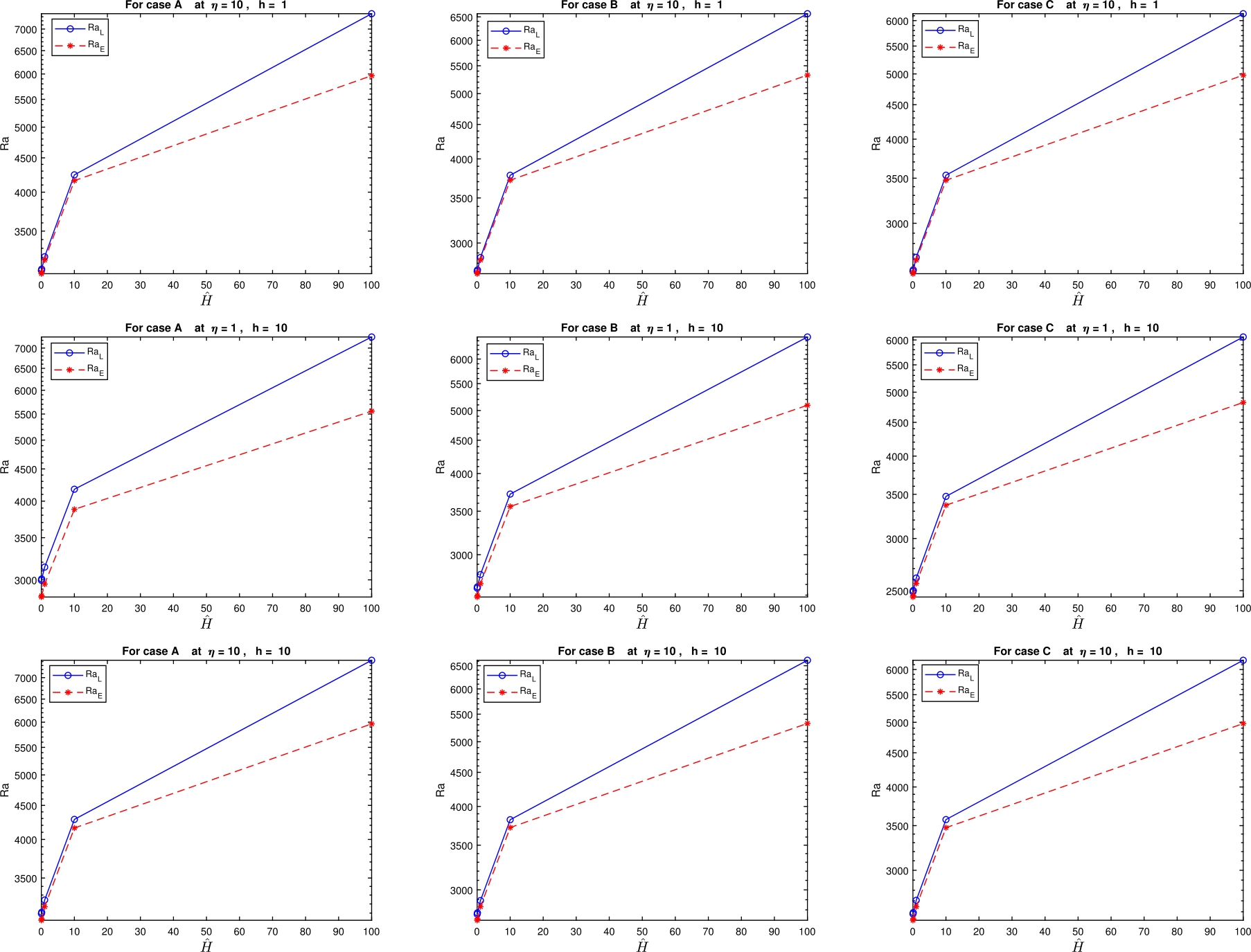
In Table 2, we list the results for various values of λ ˆ with fixed R s 2 = 5 , γ ˜ = 1 , A ˆ = 1 , H ˆ = 1 , and ζ = 0.6 at η > h , η < h , and η = h . When λ ˆ increases, the critical Rayleigh number decreases, and we notice a subcritical stability region as there is a difference between the critical Rayleigh numbers of linear and nonlinear theories when λ ˆ = 100 , particularly when η < h , as seen in Figure 3.

$Figure 3 The critical Rayleigh number of linear instability and nonlinear stability threshold for η > h \eta >h , η < h \eta <h , η = h \eta =h , R s 2 = 5 {R_{s}^{2}}=5 , γ ˜ = 1 \tilde{\gamma }=1 , A ˆ = 1 \hat{\mathcal{A}}=1 , H ˆ = 1 \hat{H}=1 , and ζ = 0.6 \zeta =0.6 , for various values of λ ˆ \hat{\lambda } .$

Figure 3

The critical Rayleigh number of linear instability and nonlinear stability threshold for η > h , η < h , η = h , R s 2 = 5 , γ ˜ = 1 , A ˆ = 1 , H ˆ = 1 , and ζ = 0.6 , for various values of λ ˆ .

For different values of ζ, with the reaction rates η > h , η < h , η = h , and fixed values of R s 2 = 5 , γ ˜ = 1 , A ˆ = 1 , H ˆ = 1 , and λ ˆ = 0.5 , the results in Table 3 clearly illustrate that the heat parameter ζ is destabilizing the system where the values of R a L and R a E rapidly decrease as ζ grows, for instance, as η = 10 , h = 1 , for case A, R a L = 1895.276 , R a E = 1882.406 at ζ = 1 , whereas at ζ = 10 , R a L = 188.883 , R a E = 131.078 . The same qualitative behavior is also seen in the other cases and situations considered, e. g., η = 1 , h = 10 , and η = 10 , h = 10 , which are depicted in Figure 4. However, a small subcritical stability region is found where there is a difference between R a L and R a E boundaries when the value of h is bigger than the value of η.

Table 3

Critical Rayleigh numbers of linear theory R a L and nonlinear energy theory R a E , corresponding to critical wave numbers a c for η > h , η < h , η = h , R s 2 = 5 , γ ˜ = 1 , A ˆ = 1 , H ˆ = 1 , and λ ˆ = 0.5 , for various values of ζ.

	Case A				Case B				Case C

ζ	R a L	a c L	R a E	a c E	R a L	a c L	R a E	a c E	R a L	a c L	R a E	a c E
η = 10 , h = 1
10 − 1	19505.371	3.485	16168.005	3.430	11961.931	3.262	11074.361	3.273	9304.902	3.238	8752.438	3.251
1	1895.276	3.174	1882.406	3.175	1766.540	3.173	1755.796	3.173	1694.087	3.173	1683.118	3.173
10	188.883	3.168	131.078	3.170	187.565	3.168	129.645	3.170	186.754	3.168	128.762	3.170
10 2	22.231	3.125	20.821	3.873	22.218	3.124	20.811	3.873	22.210	3.124	20.794	3.873
η = 1 , h = 10
10 − 1	19378.291	3.475	15493.601	3.313	11847.481	3.251	10507.580	3.145	9202.435	3.225	8291.297	3.122
1	1847.661	3.148	1771.779	3.043	1720.641	3.146	1652.520	3.041	1649.190	3.145	1584.194	3.041
10	175.090	3.090	115.412	3.000	173.828	3.090	114.060	3.000	173.051	3.090	113.225	3.000
10 2	28.828	3.495	17.300	3.873	28.813	3.495	17.287	3.873	28.804	3.495	17.268	3.873
η = 10 , h = 10
10 − 1	19584.525	3.489	16167.768	3.430	12031.421	3.267	11074.273	3.273	9367.056	3.243	8752.376	3.251
1	1924.629	3.186	1882.382	3.175	1794.881	3.185	1755.774	3.173	1721.839	3.185	1683.096	3.173
10	198.315	3.207	131.076	3.170	196.964	3.207	129.643	3.170	196.133	3.207	128.760	3.170
10 2	25.635	3.263	19.893	3.873	25.621	3.263	19.884	3.873	25.612	3.263	19.869	3.873

$Figure 4 The critical Rayleigh number of linear instability and nonlinear stability threshold for η > h \eta >h , η < h \eta <h , η = h \eta =h , R s 2 = 5 {R_{s}^{2}}=5 , γ ˜ = 1 \tilde{\gamma }=1 , A ˆ = 1 \hat{\mathcal{A}}=1 , H ˆ = 1 \hat{H}=1 , and λ ˆ = 0.5 \hat{\lambda }=0.5 , for various values of ζ.$

Figure 4

The critical Rayleigh number of linear instability and nonlinear stability threshold for η > h , η < h , η = h , R s 2 = 5 , γ ˜ = 1 , A ˆ = 1 , H ˆ = 1 , and λ ˆ = 0.5 , for various values of ζ.

In the case of the reaction rates η > h and η < h and fixed values of γ ˜ = 1 , A ˆ = 0.5 , H ˆ = 1 , λ ˆ = 0.5 , and ζ = 0.6 , analyzing the influence of various values of the salt Rayleigh number R s 2 on the stability boundary demonstrates that increasing the value of salt Rayleigh number R s 2 leads to an increasing value of the linear instability, and the difference between the linear instability and energy stability values will be considerable, especially as η < h , the gap between R a L and R a E thresholds widens, as show in Figure 5.

$Figure 5 The critical Rayleigh number of linear instability and nonlinear stability threshold for η > h \eta >h , η < h \eta <h , γ ˜ = 1 \tilde{\gamma }=1 , A ˆ = 0.5 \hat{\mathcal{A}}=0.5 , H ˆ = 1 \hat{H}=1 , λ ˆ = 0.5 \hat{\lambda }=0.5 , and ζ = 0.6 \zeta =0.6 , for various values of R s 2 {R_{s}^{2}} .$

Figure 5

The critical Rayleigh number of linear instability and nonlinear stability threshold for η > h , η < h , γ ˜ = 1 , A ˆ = 0.5 , H ˆ = 1 , λ ˆ = 0.5 , and ζ = 0.6 , for various values of R s 2 .

7 Conclusions

In this article, the problem of thermosolutal convection in a porous medium of Darcy–Brinkman model where the layer is heated and salted from below is studied. We have investigated in detail the reaction and thermal non-equilibrium effects with three basic forms of the internal heat source. The linear instability and nonlinear stability theories were applied to investigate the effect of various parameters on the stability of the system. Numerical results were achieved by using the D 2 Chebyshev tau method. The following conclusions can be stated:

It could be argued based on the results that the interphase heat transfer parameter H ˆ for fixed values of R s 2 , γ ˜ , A ˆ , λ ˆ , and ζ, when η > h , η < h , and η = h , for all cases of the internal heat source, has a stabilizing effect on the system. Also, it is observed that a small subcritical stability area may arise for h larger than η.
For all cases of the internal heat source, the porosity modified conductivity ratio λ ˆ and heat parameter ζ, for fixed values of R s 2 , γ ˜ , A ˆ , and H ˆ at η > h , η < h , and η = h , play important roles in the stability and instability regions.
The salt Rayleigh number R s 2 , for fixed values of γ ˜ , A ˆ , H ˆ , λ ˆ , and ζ whenever η > h or η < h , for all cases of the internal heat source, is an important factor in determining whether a region is stable or unstable.

References

[1] B. Straughan, Porous convection with local thermal non-equilibrium temperatures and with Cattaneo effects in the solid, Proc. R. Soc. A, Math. Phys. Eng. Sci., 469 (2013), no. 2157, 20130187.10.1098/rspa.2013.0187Search in Google Scholar

[2] M. Celli, A. Barletta and L. Storesletten, Local thermal non-equilibrium effects in the Darcy–Bénard instability of a porous layer heated from below by a uniform flux, Int. J. Heat Mass Transf. 67 (2013), 902–912.10.1016/j.ijheatmasstransfer.2013.08.080Search in Google Scholar

[3] S. Choudhary, A. Mahajan, et al., Conditional stability for thermal convection in a rotating couple-stress fluid saturating a porous media with temperature- and pressure-dependent viscosity using a thermal non-equilibrium model, J. Non-Equilib. Thermodyn. 39 (2014), no. 2, 61–78.10.1515/jnetdy-2013-0025Search in Google Scholar

[4] B. Straughan, Convection with Local Thermal Non-equilibrium and Microfluidic Effects, vol. 32, Springer, 2015.10.1007/978-3-319-13530-4Search in Google Scholar

[5] B. Straughan, Exchange of stability in Cattaneo–LTNE porous convection, Int. J. Heat Mass Transf. 89 (2015), 792–798.10.1016/j.ijheatmasstransfer.2015.05.084Search in Google Scholar

[6] M. Celli, A. Barletta and D. Rees, Local thermal non-equilibrium analysis of the instability in a vertical porous slab with permeable sidewalls, Transp. Porous Media 119 (2017), no. 3, 539–553.10.1007/s11242-017-0897-xSearch in Google Scholar

[7] I. M. Mankhi and S. A. Haddad, Effect of local thermal non-equilibrium on the onset of convection in an anisotropic bidispersive porous layer, J. Al-Qadisiyah Computer Sci. Math. 13 (2021), no. 2, 181–192.Search in Google Scholar

[8] F. Capone and J. A. Gianfrani, Thermal convection for a Darcy–Brinkman rotating anisotropic porous layer in local thermal non-equilibrium, Ric. Mat. 71 (2022), no. 1, 227–243.10.1007/s11587-021-00653-6Search in Google Scholar

[9] A. Nouri-Borujerdi, A. R. Noghrehabadi and D. A. S. Rees, The effect of local thermal non-equilibrium on conduction in porous channels with a uniform heat source, Transp. Porous Media 69 (2007), no. 2, 281–288.10.1007/s11242-006-9064-5Search in Google Scholar

[10] A. Nouri-Borujerdi, A. R. Noghrehabadi and D. A. S. Rees, Influence of Darcy number on the onset of convection in a porous layer with a uniform heat source, Int. J. Therm. Sci. 47 (2008), no. 8, 1020–1025.10.1016/j.ijthermalsci.2007.07.014Search in Google Scholar

[11] A. Kuznetsov and D. Nield, Local thermal non-equilibrium and heterogeneity effects on the onset of convection in an internally heated porous medium, Transp. Porous Media 102 (2014), no. 1, 15–30.10.1007/s11242-013-0258-3Search in Google Scholar

[12] A. Mahajan and R. Nandal, Anisotropic porous penetrative convection for a local thermal non-equilibrium model with Brinkman effects, Int. J. Heat Mass Transf. 115 (2017), 235–250.10.1016/j.ijheatmasstransfer.2017.08.034Search in Google Scholar

[13] A. Mahajan and R. Nandal, Penetrative convection in a fluid saturated Darcy–Brinkman porous media with LTNE via internal heat source, Nonlinear Eng. 8 (2019), no. 1 546–558.10.1515/nleng-2018-0053Search in Google Scholar

[14] C. Siddabasappa and T. Sakshath, Effect of thermal non-equilibrium and internal heat source on Brinkman–Bénard convection, Physica A 566 (2021), 125617.10.1016/j.physa.2020.125617Search in Google Scholar

[15] R. Sharma and M. Pal, Hall effect on thermosolutal instability of a Rivlin–Ericksen fluid in a porous medium, J. Non-Equilib. Thermodyn. 26 (2001), no. 4, 373–386.10.1515/JNETDY.2002.024Search in Google Scholar

[16] D. Pritchard and C. N. Richardson, The effect of temperature-dependent solubility on the onset of thermosolutal convection in a horizontal porous layer, J. Fluid Mech. 571 (2007), 59–95.10.1017/S0022112006003211Search in Google Scholar

[17] S. Wang and W. Tan, The onset of Darcy–Brinkman thermosolutal convection in a horizontal porous media, Phys. Lett. A 373 (2009), no. 7, 776–780.10.1016/j.physleta.2008.12.056Search in Google Scholar

[18] I. C. Liu and J. Umavathi, Double diffusive convection of a micropolar fluid saturated in a sparsely packed porous medium, Heat Transf. Asian Res. 42 (2013), no. 6, 515–529.10.1002/htj.21052Search in Google Scholar

[19] A. Mahajan and V. K. Tripathi, Stability of a chemically reacting double-diffusive fluid layer in a porous medium, Heat Transf. 50 (2021), no. 6, 6148–6163.10.1002/htj.22166Search in Google Scholar

[20] N. J. Noon and S. Haddad, Stability analysis for rotating double-diffusive convection in the presence of variable gravity and reaction effects: Darcy model, Spec. Top. Rev. Porous Media Int. J. 13 (2022), no. 4.10.1615/SpecialTopicsRevPorousMedia.2022042776Search in Google Scholar

[21] M. Malashetty, M. Swamy and R. Heera, Double diffusive convection in a porous layer using a thermal non-equilibrium model, Int. J. Therm. Sci. 47 (2008), no. 9, 1131–1147.10.1016/j.ijthermalsci.2007.07.015Search in Google Scholar

[22] M. Malashetty and R. Heera, Linear and non-linear double diffusive convection in a rotating porous layer using a thermal non-equilibrium model, Int. J. Non-Linear Mech. 43 (2008), no. 7, 600–621.10.1016/j.ijnonlinmec.2008.02.006Search in Google Scholar

[23] X. Chen, S. Wang, J. Tao and W. Tan, Stability analysis of thermosolutal convection in a horizontal porous layer using a thermal non-equilibrium model, Int. J. Heat Fluid Flow 32 (2011), no. 1, 78–87.10.1016/j.ijheatfluidflow.2010.06.003Search in Google Scholar

[24] M. Malashetty, A. A. Hill and M. Swamy, Double diffusive convection in a viscoelastic fluid-saturated porous layer using a thermal non-equilibrium model, Acta Mech. 223 (2012), no. 5, 967–983.10.1007/s00707-012-0616-1Search in Google Scholar

[25] D. Nield, A. Kuznetsov, A. Barletta and M. Celli, The effects of double diffusion and local thermal non-equilibrium on the onset of convection in a layered porous medium: non-oscillatory instability, Transp. Porous Media 107 (2015), no. 1, 261–279.10.1007/s11242-014-0436-ySearch in Google Scholar

[26] A. Kuznetsov, D. Nield, A. Barletta and M. Celli, Local thermal non-equilibrium and heterogeneity effects on the onset of double-diffusive convection in an internally heated and soluted porous medium, Transp. Porous Media 109 (2015), no. 2, 393–409.10.1007/s11242-015-0525-6Search in Google Scholar

[27] A. Altawallbeh, I. Hashim and A. Tawalbeh, Thermal non-equilibrium double diffusive convection in a Maxwell fluid with internal heat source, Journal of Physics: Conference Series 1132 (2018), 012027.10.1088/1742-6596/1132/1/012027Search in Google Scholar

[28] C. H. Kumar, B. Shankar and I. Shivakumara, Weakly nonlinear stability of thermosolutal convection in an Oldroyd-b fluid-saturated anisotropic porous layer using a local thermal non-equilibrium model, J. Heat Transf. 144 (2022), no. 7, 072701.10.1115/1.4054123Search in Google Scholar

[29] C. Hemanth Kumar, B. Shankar and I. Shivakumara, Thermosolutal LTNE porous mixed convection under the influence of the Soret effect, J. Heat Transf. 144 (2022), no. 4, 042602.10.1115/1.4053331Search in Google Scholar

[30] B. Straughan, The Energy Method, Stability, and Nonlinear Convection, vol. 91, Springer Science & Business Media, 2004.10.1007/978-0-387-21740-6Search in Google Scholar

[31] S. Chandrasekhar, Hydrodynamic and Hydromagnetic Stability, Courier Corporation, 2013.Search in Google Scholar

[32] J. Dongarra, B. Straughan and D. Walker, Chebyshev tau-QZ algorithm methods for calculating spectra of hydrodynamic stability problems, Appl. Numer. Math. 22 (1996), no. 4, 399–434.10.1016/S0168-9274(96)00049-9Search in Google Scholar

Received: 2022-07-05

Accepted: 2022-08-26

Published Online: 2022-09-20

Published in Print: 2023-01-27

Articles in the same Issue

https://doi.org/10.1515/jnet-2022-0047

Keywords for this article

stability analysis; double diffusive convection; internal heat source effect; reaction effect; Darcy–Brinkman model; local thermal non-equilibrium; porous media