
Stochastic methods defeat regular RSA exponentiation algorithms with combined blinding methods
-
Margaux Dugardin

Abstract
Extra-reductions occurring in Montgomery multiplications disclose side-channel information which can be exploited even in stringent contexts. In this article, we derive stochastic attacks to defeat Rivest-Shamir-Adleman (RSA) with Montgomery ladder regular exponentiation coupled with base blinding. Namely, we leverage on precharacterized multivariate probability mass functions of extra-reductions between pairs of (multiplication, square) in one iteration of the RSA algorithm and that of the next one(s) to build a maximum likelihood distinguisher. The efficiency of our attack (in terms of required traces) is more than double compared to the state-of-the-art. In addition to this result, we also apply our method to the case of regular exponentiation, base blinding, and modulus blinding. Quite surprisingly, modulus blinding does not make our attack impossible, and so even for large sizes of the modulus randomizing element. At the cost of larger sample sizes our attacks tolerate noisy measurements. Fortunately, effective countermeasures exist.
1 Introduction
It has been noted by Kocher [13] as early as 1996 that asymmetric cryptographic algorithms are prone to side-channel attacks. Countermeasures have been developed in a view to make these attacks either impossible or at least much harder to perform. There are several countermeasure principles. One first class consists in balancing the control-flow so that execution traces perfectly superimpose whatever the value of the secrets. A second important class of countermeasures consists in deceiving correlation attempts by attacker with side-channel traces. The strategy consists in randomizing algorithm inputs or internal parameters, so that the computation is carried out on unpredictable data. Obviously, the randomization is restricted, since it must be possible to unravel the injected randomness at the end of the computation.
In this article, we focus on the Rivest-Shamir-Adleman (RSA) cryptosystem, while it uses its secret exponent
In practice, the attacks which succeed in a single trace are the more dangerous, and implementers defend their implementation in the first place. The so-called simple power analysis (SPA [14, §2]) introduced in 1999 allows us to read out the exponent in one trace. Therefore, the usual countermeasure consists in the implementation of a regular exponentiation algorithm. In RSA, the so-called “regular algorithm” is a method to compute the modular exponentiation using a key-independent sequence of squaring and multiplication operations. Examples of regular exponentiation algorithms are the Montgomery ladder (treated in this paper), the square and multiply always algorithm, or fixed window exponentiation with explicit multiplication also if the exponent bits in the current window are all equal to zero [15, Algorithm 14.82].
Thus, it is a protection against the simple trace analysis, where the attacker attempts to derive the exponent by observing one (or several identical) computation. The regular exponentiation countermeasure against SPA plugs the leak, but in the meantime takes care to properly align traces corresponding to various executions. This is at the advantage of the adversary, in that such unfortunate alignment opens the door to differential power analyses, as discussed in [14, §5], to template attacks [5], or to machine learning attacks [19]. Those attacks, provided they require to collect several traces from the same inputs (for averaging in order to increase the SNR), are combated by randomizing countermeasures. For instance, the input of the RSA (its base) can be randomized at the input, while being consistently derandomized at the output. Another option to randomize the intermediate computations is to randomize the modulus (so-called “modular extension”). This second option also allows us to perform a sanity check for the computation, which is incidentally a countermeasure against fault injection attacks [7]. We insist that all three countermeasures might well be stacked one on top of each other, so as to thwart simple power attacks, differential power attacks, and perturbation attacks, altogether. As an alternative to regular exponentiation algorithm, or even as a complement to it, the secret exponent can be protected by blinding, as explained earlier.
2 Previous work and our contributions
2.1 State-of-the-art
We analyze in this article possible remaining biases, namely, extra-reductions inherent to the modular multiplication algorithm.
Given two integers
Definition 2.1
(Montgomery Transformation [16]) For any modulus
In order to ease the computation,
Definition 2.2
(MMM [16]) Let
Proposition 2.3
(MMM correction [15, §14.36]) The output of the MMM of
Algorithm 1 shows that the MMM can be implemented in two steps:
compute
reduce
Algorithm 1
|
input :
|
|
output :
|
|
1
|
|
2
|
|
3
if
|
|
4
|
|
5
|
|
6
return
|
Montgomery reduction (Algorithm 14.32 of [15])
Definition 2.4
(Extra-reduction) In Algorithm 1, when the intermediate value
As we shall explain, this side channel is induced by the choice of moduli represented on a bitwidth, which is exactly divisible by the bitwidth of the computers, namely, this bitwidth is typically a power of two, such as 16, 32, or 64. This bias has given rise to the so-called extra-reduction analysis (ERA). An overview of known ERAs is provided in Table 1. Specifically, this table shows which countermeasure can be bypassed by which attack. The classification criteria in Table 1 are listed as follows:
the implementation uses the Chinese Remainder Theorem (CRT), i.e., the moduli
the protection against differential power analysis named the base blinding,
the protection against SPA protection named the regular exponentiation algorithm,
the compensation of the extra-reduction by a fake operation, which is named constant time nonstraight line algorithm (N-SLA), i.e., constant operations have their fixed values identified by software.[2] In principle (at least with a reasonable probability), these countermeasures might be detected and nullified by a suitable side-channel attack. In Table 1, we assume that such side-channel attacks exist,
the protection against differential power analysis named the exponent blinding, and
the fault and differential protection named modular extension.
Summary of capability of extra-reduction analyses published before December 2020
| With RSA-CRT | Basis blinding | Regular algorithm | Constant time N-SLA | Constant time SLA | Exponent blinding | Modular extension | |
|---|---|---|---|---|---|---|---|
| ERA-1a | ✗ | ✗ | ✗ | ✗ | ✗ | ✗ | ✗ |
| [9,13,22,25] | No | No | No | No | No | No | No |
| ERA-1b | ✓ | ✗ | ✓ | ✗ | ✗ | ✗ | ✗ |
| [3,6,8,20] | Yes | No | Yes | No | No | No | No |
| ERA-2 | ✓ | ✗ | ✗ | ✗ | ✗ | ✓ | ✗ |
| [23,24] | Yes | No | No | No | No | Yes | No |
| ERA-L1 | ✓ | ✓ | ✓ | ✗ | ✗ | ✗ | ✗ |
| [1,2,21,26,30] | Yes/No | Yes | Yes | No | No | No | No |
| ERA-L2 | ✓ | ✓ | ✓ | ✓ | ✗ | ✗ | ✗ |
| [10,11] | Yes/No | Yes | Yes | Yes | No | No | No |
| This work | ✓ | ✓ | ✓ | ✓ | ✗ | ✗ | ✓ |
| Yes/No | Yes | Yes | Yes | No | No | Yes |
The algorithms from ERA-1a, ERA-1b, and ERA-2 are pure (global) timing attacks. Of course, by definition, pure timing attacks cannot overcome constant time implementations. While the pure timing attacks are very different for CRT implementations and for non-CRT implementations the local timing attacks from ERA-L1 and ERA-L2 work for the CRT and non-CRT implementations as well. More precisely, these local attacks are a little bit easier to perform on non-CRT implementations because the ratio
Remark
The terminology in Table 1 shall be considered with attention. Indeed, historically, ERA-1a, ERA-1b, and ERA-2 are pure timing attacks discovered in this order. Similarly, ERA-L1 and ERA-L2 are local timing attacks, discovered in this order. But some papers about ERA-1b were published after the papers from ERA-L1 and vice versa.
In [10,11], side-channel attacks on RSA, with CRT and without CRT, were investigated using leakage information of the presence or absence of the extra-reductions in MMM. The side-channel information was used to identify, which MMs require extra reductions. Two exponentiation algorithms were considered, namely, the always square and multiply exponentiation and the Montgomery ladder. The overall attacks split into many individual decisions whether
2.2 Novel contributions
For these reasons, in this article, we resort to another way to estimate the distribution of the extra-reduction which does not need the estimation of PMF values. We leverage on a previous work of Schindler [21]: this paper simplifies the characterization of the extra-reduction distribution using two elegant properties of MMM.
Using sophisticated stochastic methods, we solve the problem and improve the efficiency of [10,11], in the presence of regular exponent and base blinding.
Moreover, we extend the results to the case where the modulus is itself randomized. We show that ERA remains a powerful side-channel despite the stacking of three protections, namely, regular exponentiation and base and modulus blinding. We performed our experiments on 1024-bit RSA moduli as this allows a fair comparison of the attack efficiency with the experimental results in [10,11].
This manuscript contains joint research work from the years 2016–2018. We mention that parts of an intermediate version of this paper have found input in the PhD thesis of the lead author.
2.3 Outline
The rest of this paper is organized as follows. We start by giving our optimized attack in Section 3. Namely, we recapitulate in Section 3.1 the background to optimize the state-of-the-art when RSA uses a regular algorithm (we focus on the so-called Montgomery ladder) and base blinding. The core of our attack is presented in Section 3.2. Evaluation with both perfect and noisy measurements is conducted in Section 4, where we also consider the “modulus extension” as a third countermeasure on top of regular exponentiation and base blinding. Eventually, countermeasures are addressed in Section 5, and conclusions are derived in Section 6. Some formal computation results are given in Appendix 7.
3 The optimized attack: the stochastic background
In this section, we optimize the attack from [10,11]. We begin with definitions and we formulate the target of our attack in Section 3.1. In Section 3.2, we analyze the stochastic properties of the MM, and in Lemma 3.4 we develop a formula for the joint probability of several extra-reductions. The following subsections treat the estimation of two parameters, which are usually unknown, and the maximum likelihood estimator is derived.
3.1 Definitions and target of the attack
In this paper, we only consider the Montgomery ladder (left-to-right), which is described in Algorithm 2. Unlike [10,11] we do not consider the square and always multiply algorithm (cf. Algorithm 1.1 in [11]). It is obvious how the applied mathematical methods can be transferred to the square and always multiply exponentiation algorithm.
We assume that the message
To avoid clumsy formulations we always target RSA with CRT in the following, where
Definition 3.1 describes the notations, necessary to understand this paper.
Definition 3.1
For
Algorithm 2
|
Input:
|
|
Output:
|
|
1
|
|
2
|
|
3
for
|
|
|
|
6
return
|
Left-to-right Montgomery ladder with MM algorithm
We note that
3.2 The core of our attack
We interpret the
Lemma 3.2
(MM)
- (3.1)
Assume that
(3.2)(3.3)The random variables
For
(3.4)(3.5)For the indicator functions, we obtain
(3.6)(3.7)
Proof
Assertions (i) and (ii) are shown in [22] (see Lemma A.3 and its proof at page 209). The core idea of the approximate representations (3.2) and (3.3) is that a small deviation of the random variable
Remark 3.3
(The independence assumption) A central assertion of Lemma 3.2, which is used in Lemma 3.4, is that random variables
The overall attack consists of many independent decisions (which nevertheless influence each other). Each of these attack steps (decisions) considers all MM simultaneously, which are carried out when
Lemma 3.4
Let
The term (3.8) quantifies the probability that the extra-reduction vector
(3.8)Note: When the key bit
If
(3.9)(3.10)If
(3.11)and
(3.12)Let
(3.13)(3.14)
Proof
By Lemma 3.2(iv), the random variables
with suitable integration boundaries
We first note that
(swapping the right-hand indices from 0 to 1 and vice versa) defines a volume-preserving diffeomorphism on
and
respectively. The terms
Lemma 3.4(ii) says that the information contained in the extra-reduction vectors

Information collected during the presented attack on
In particular, it would be pointless to consider the case
where “
Remark 3.5
Lemma 3.4 can be applied to all
The probabilities in Lemma 3.4 do not depend on the index
For
Example 3.6
Let
Corollary 3.7
For
Remark 3.8
The two approaches in previous work [10, 11] and this work are independent and both allow us to derive a maximum likelihood key distinguisher. Here, we are not interested in the values manipulated by the multiplication and square operations, but only with the necessary and sufficient conditions for the existence of extra-reductions, allowing an analysis of larger dimensions.
4 Perfect and noisy measurements
The attacker gets access to side-channel information about each bit
Thus, the attacker garners an iid sequence
In practical cases, detecting an extra-reduction using only one acquisition can lead to errors. Let us model the attack setup, taking into account that the detection of presence/absence of extra-reductions is a random variable, due to some noise. The random variables Markov chain for index
| Secret |
|
Bias |
|
Observable |
|---|---|---|---|---|
|
|
|
|
|
|
The probabilities (3.8) depend on the unknown ratio
Lemma 4.1
It is
Proof
Since
We note that the probability (4.2) was already verified in [20][3] and, for instance, in [11], respectively, the latter by other mathematical methods. Formula (4.3) follows directly from (4.1) and (4.2).□
The ER-values
and similarly for the initialization of the registers
Lemma 4.2
Proof
Since
and similarly
Solving these equations for
In Lemma 4.3,
Lemma 4.3
- (4.7)
For each hypothesis
(4.8)
Proof
The term
The last lemma of this section explains how to estimate the ratio
Lemma 4.4
Assume that the attacker has observed
provides an estimator for
for
(iii) For perfect measurements alternatively (4.3) might be used to estimate
Proof
Straightforward.□
Example 4.5
(Estimation of

Statistic box plot to estimate the ratio

Success rate for an entire exponent using 1.000 randomly selected exponent values depending on the number of side-channel traces
4.1 The optimal decision strategy
Lemma 4.6 provides the optimal decision strategy for the individual decisions, i.e., for guessing the parameter set
Lemma 4.6
(Maximum likelihood estimator) Assume that the key
The attacker decides for
(4.12)This is the optimal decision strategy.
Proof
The first assertion of (i) follows from Lemma 3.4(ii), and the second is an immediate consequence of the first. With regard to the assumptions on
Remark 4.7
In the proof of Lemma 4.6, we assume that
In the proof of Lemma 4.6, we assume that each false decision is equally bad. This assumption is reasonable if all transformed subkeys
are treated independently.
4.2 Attack summary and success rate
The decision strategy in Lemma 4.6 is based on the observed extra-reductions for each multiply and square operation for
the attacker estimates the
The last steps of Algorithm 3 consist in putting together pieces of
Algorithm 3
|
Input:
|
|
|
Output: A guessed key value
|
|
| Attack phase | |
| 1 | Estimate the ratio
|
| 2 |
for each
|
| 3 |
|
| 4 |
for
|
|
|
|
| Computation of the estimated key value | |
|
|
|
|
|
for
|
|
|
|
|
|
return
|
Optimal extra-reduction attack using maximum likelihood estimator
In order to compare the previous work and this optimized method, we compute the success rate of those attacks. In this article, we define the success rate of a whole exponent value.
Definition 4.8
(Success rate of an attack) The success rate of an attack is the number of succeeded attacks over the number of experiments. The attack succeeds when all the key bits of entire exponent are found. As a corollary, if only one bit is badly guessed, then the attack is considered to have failed.
For different exponents of 512-bit length, we estimate the success rate of the attack for the modulo (RSA-1024-q defined in [11, Section 2.2]), for different probabilities
The gain obtained by the increasing
4.3 The attack in the presence of several blinding techniques
We already know that base blinding (a.k.a. message blinding) does not prevent our attack. The reason is that our attack neither requires the knowledge of any register values
4.3.1 The combination of basis blinding with modulus blinding
In the first step, an odd modulus blinding factor
Remark 4.9
The modulus blinding factor
Of course, the annihilating term
In this paper, we consider the case “first modulus blinding then base blinding.” This countermeasure is represented in Algorithm 5. We point out that reversed order, “first base blinding then modulus blinding,” can be attacked in the same way.
Algorithm 4
|
Input:
|
|
Output:
|
|
1
|
|
2
|
|
3
|
|
4
for
|
|
|
|
7
return
|
Left-to-right Montgomery ladder exponentiation built on top of MM algorithm, with base blinding (attacked in this paper, in Section 4.1)
Algorithm 5
|
Input:
|
|
Output:
|
|
1
|
|
2
|
|
3
|
|
4
|
|
5
for
|
|
|
|
8
return
|
Left-to-right Montgomery ladder exponentiation built on top of MM algorithm, with base and modulus blinding (attacked in this paper, in Section 4.3). (Throughout this algorithm, the MM algorithm uses
For the case that only base blinding (or even no blinding technique at all) is applied, Lemma 3.4 provides concrete formulae that the extra-reduction vector
In this subsection, the ratio between the modulus and the Montgomery constant is no longer constant but depends on the selected modulus blinding value
However, the applied modulus blinding factor
quantifies the probability for the extra-reduction vector
Usually the normalized blinding factors should be uniformly distributed on
For reasonable parameter
In analogy to Section 4, the next step is to estimate
Substituting
More precisely, a careful computation yields
The right-hand side of (4.18) differs from (4.5) by the factor
Above we have identified two strategies for the selection of modulus blinding factors, which are of particular interest. If
Substituting (4.13) (resp., (4.14) or (4.15)) into Lemma 4.3(i) yields analogous assertions for the modulus blinding case. The estimation of
Altogether, modulus blinding does not prevent our attack. For power trace
Remark 4.10
Alternatively to the attack just analyzed one might estimate the product
4.3.2 Experimental results with modulus blinding
Figure 4 compares the success rate evolution of our attack, using (4.14), for the same three noise levels as in Figure 3, for

Success rate for an entire exponent depending on the number of side-channel trace
It can be seen that the value of
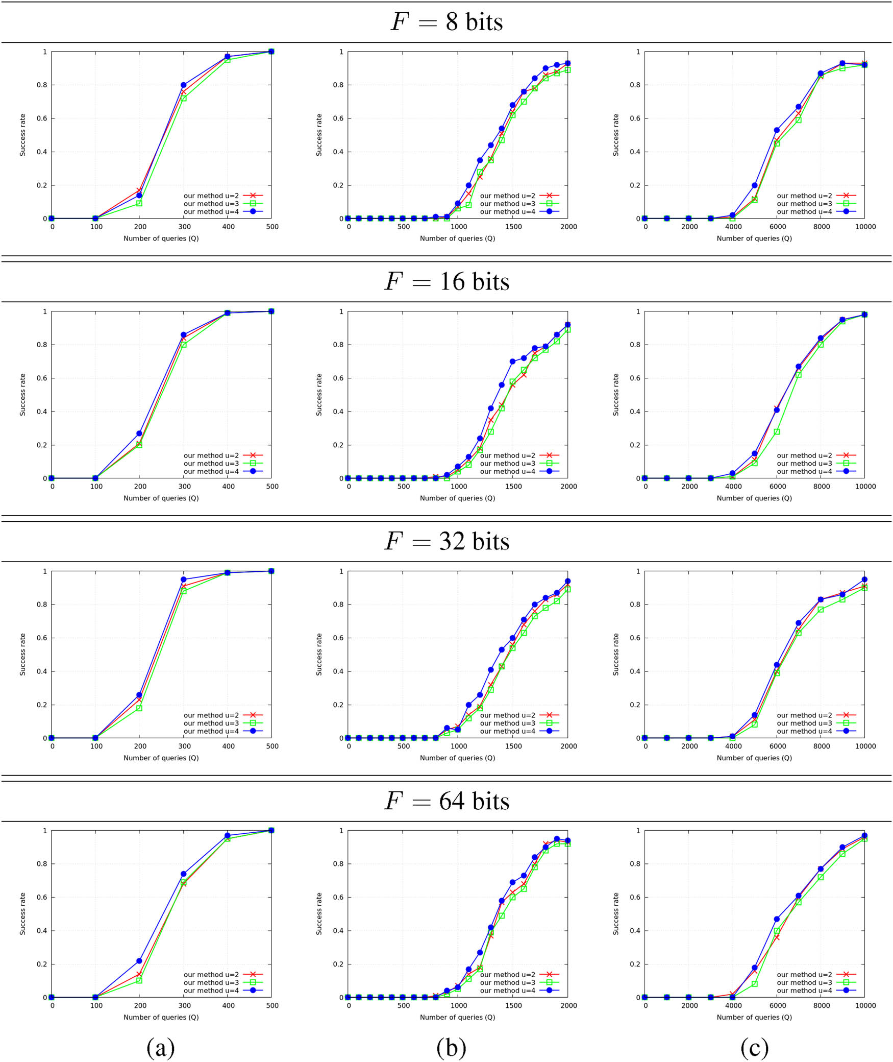
Success rate for an entire exponent depending of the number of side-channel trace
The success rate for some modulus randomization factors
when
when
when
4.3.3 The combination of basis blinding with exponent blinding
Assume that base blinding is combined with (additive) exponent blinding, which means that the exponent
It should be noted, however, that if (e.g.) single-trace template attacks provide significant advantage over blind guessing of the exponent bits
5 Countermeasures
In Table 1 and in Section 4.3, several countermeasures were addressed and analyzed. In particular, even the combination of base blinding and exponent blinding does not prevent our attack. An option is to add exponent blinding, resulting in the combination (base blinding and exponent blinding) or in (base blinding, modulus blinding, and exponent blinding). In the absence of additional leakage, to our best knowledge no attack is known (Section 4.3).
The most solid solution, of course, is to avoid extra-reductions at all. Following an idea of C. Walter one can completely resign on extra-reductions if the Montgomery constant
6 Conclusion
In [10,11], ERA exploiting the dependency of two consecutive MMs was applied to attack RSA implementations, which use the Montgomery ladder or the always square and multiply exponentiation algorithm. Basis blinding does not prevent this attack. Although both attacks were successful they did not exploit all the available information. In this paper, we followed the strategy in [1,2,21], formulated, and analyzed a stochastic process, which was tailored to the stochastic behavior of the extra-reductions in Montgomery ladder. This sophisticated strategy allowed us to exploit all the given information in an optimal way. Practical experiments underlined that the new method reduces the sample size by a factor greater than 2 (to
Acknowlegments
This work has benefited from a partial funding via TeamPlay (https://teamplay-h2020.eu/), a project from European Union’s Horizon 2020 research and innovation program, under grant agreement no. 779882. The analysis methods have been integrated into Secure-IC Laboryzr tools.
Appendix A
Tables A.1 and A.2 contain all probabilities for
|
|
|
|||
|---|---|---|---|---|
| (0,0) | (0,1) | (1,0) | (1,1) | |
| (0,0) |
|
|
|
|
| (0,1) |
|
|
|
|
| (1,0) |
|
|
|
|
| (1,1) |
|
|
|
|
|
|
|
|||
|---|---|---|---|---|
| (0,0) | (0,1) | (1,0) | (1,1) | |
| (0,0) |
|
|
|
|
| (0,1) |
|
|
|
|
| (1,0) |
|
|
|
|
| (1,1) |
|
|
|
|
References
[1] Acıiçmez O, Schindler W. A major vulnerability in RSA implementations due to microarchitectural analysis threat. IACR Cryptology ePrint Archive 2007;2007:336. Search in Google Scholar
[2] Acıiçmez O, Schindler W. A vulnerability in RSA implementations due to instruction cache analysis and its demonstration on OpenSSL. In: Malkin T, editor. Topics in Cryptology – CT-RSA 2008, Proceedings of the Cryptographers’ Track at the RSA Conference 2008, San Francisco, CA, USA, April 8–11, 2008. Lecture Notes in Computer Science, vol. 4964, Springer; 1997. p. 256–73. 10.1007/978-3-540-79263-5_16Search in Google Scholar
[3] Acıiçmez O, Schindler W, Koç ÇK. Improving Brumley and Boneh timing attack on unprotected SSL implementations. In: Atluri V, Meadows C, Juels A, editors. Proceedings of the 12th ACM Conference on Computer and Communications Security, CCS 2005, Alexandria, VA, USA, November 7–11, 2005. ACM; 2005. p. 139–46. 10.1145/1102120.1102140Search in Google Scholar
[4] Akishita T, Takagi T. Zero-value point attacks on elliptic curve cryptosystem. In: Boyd C, Mao W, editors. ISC, Lecture Notes in Computer Science, vol. 2851. Springer; 2003. p. 218–33. 10.1007/10958513_17Search in Google Scholar
[5] Alam M, Khan HA, Dey M, Sinha N, Callan RL, Zajic AG, et al . One&Done: A single-decryption EM-based attack on OpenSSL’s constant-time blinded RSA. In: Enck W, Porter Felt A, editors. 27th USENIX Security Symposium, USENIX Security 2018, Baltimore, MD, USA, August 15–17, 2018, USENIX Association; 2018. p. 585–602. Search in Google Scholar
[6] Arnaud C, Fouque PA. Timing attack against protected RSA-CRT implementation used in polarssl. In: Dawson E, editor. Topics in Cryptology - CT-RSA 2013. Proceedings of the Cryptographers’ Track at the RSA Conference 2013, San Francisco, CA, USA, February 25-March 1, 2013. Lecture Notes in Computer Science, vol. 7779. Springer; 2013. p. 18–33. 10.1007/978-3-642-36095-4_2Search in Google Scholar
[7] Baek YJ, Vasyltsov I, How to prevent DPA and fault attack in a unified way for ECC scalar multiplication - ring extension method. In: Dawson Ed, Wong SW, editors. Information Security Practice and Experience, Lecture Notes in Computer Science, vol. 4464. Berlin Heidelberg: Springer; 2007. p. 225–37. 10.1007/978-3-540-72163-5_18Search in Google Scholar
[8] Brumley D, Boneh D. Remote timing attacks are practical. In: Proceedings of the 12th USENIX Security Symposium, Washington, D.C., USA, USENIX Association; August 4–8, 2003. 10.1016/j.comnet.2005.01.010Search in Google Scholar
[9] Dhem J-F, Koeune F, Leroux P-A, Mestré P, Quisquater J, Willems J-L. A practical implementation of the timing attack. In: Quisquater J-J, Schneier B, editors. Smart Card Research and Applications, Proceedings of the International Conference, CARDIS ’98, Louvain-la-Neuve, Belgium, September 14–16, 1998, Lecture Notes in Computer Science, vol. 1820. Springer; 1998p. 167–82. 10.1007/10721064_15Search in Google Scholar
[10] Dugardin M, Guilley S, Danger J-L, Najm Z, Rioul O. Correlated extra-reductions defeat blinded regular exponentiation. In: Gierlichs B, Poschmann AY, editors. Cryptographic Hardware and Embedded Systems - Proceedings of the CHES 2016 - 18th International Conference, Santa Barbara, CA, USA, August 17–19, 2016, Lecture Notes in Computer Science, vol. 9813. Springer; 2016. p. 3–22. 10.1007/978-3-662-53140-2_1Search in Google Scholar
[11] Dugardin M, Guilley S, Danger J-L, Najm Z, Rioul O. Correlated extra-reductions defeat blinded regular exponentiation - extended version. Cryptology ePrint Archive, Report 2016/597, June 6 2016. http://eprint.iacr.org/2016/597Search in Google Scholar
[12] Goubin L. A refined power-analysis attack on elliptic curve cryptosystems. In: Proceedings of the 6th International Workshop on Theory and Practice in Public Key Cryptography: Public Key Cryptography, PKC ’03. London, UK: Springer-Verlag; 2003. p. 199–210. 10.1007/3-540-36288-6_15Search in Google Scholar
[13] PC Kocher Timing attacks on implementations of diffie-hellman, RSA, DSS, and other systems. In: Koblitz N, editor. Advances in Cryptology - CRYPTO ’96, Proceedings of the 16th Annual International Cryptology Conference, Santa Barbara, California, USA, August 18–22, 1996, Lecture Notes in Computer Science, vol. 1109. Springer; 1996. p. 104–13. 10.1007/3-540-68697-5_9Search in Google Scholar
[14] Kocher PC, Jaffe J, Jun B. Differential power analysis. In: Wiener MJ, editor. CRYPTO, Lecture Notes in Computer Science, vol. 1666. Springer; 1999. p. 388–97. 10.1007/3-540-48405-1_25Search in Google Scholar
[15] Menezes AJ, van Oorschot PC, Vanstone SA. Handbook of Applied Cryptography. CRC Press; October 1996. http://www.cacr.math.uwaterloo.ca/hac/. Search in Google Scholar
[16] Montgomery PL. Modular multiplication without trial division. Math Comput. April 1985;44(170):519–21. 10.1090/S0025-5718-1985-0777282-XSearch in Google Scholar
[17] Montgomery PL. Modular multiplication without trial division. Math Comput. 1985;44(170): 519–21. 10.1090/S0025-5718-1985-0777282-XSearch in Google Scholar
[18] Nakano Y, Souissi Y, Nguyen R, Sauvage L, Danger J-L, Guilley S, Kiyomoto S, et al . A pre-processing composition for secret key recovery on android smartphone. In: Naccache D, Sauveron D, editors. Information Security Theory and Practice. Proceedings of the Securing the Internet of Things - 8th IFIP WG 11.2 International Workshop, WISTP 2014, Heraklion, Crete, Greece, June 30–July 2, 2014. Lecture Notes in Computer Science, vol. 8501. Springer; 2014. p. 76–91. 10.1007/978-3-662-43826-8_6Search in Google Scholar
[19] Perin G, Imbert L, Torres L, Maurine P. Attacking randomized exponentiations using unsupervised learning. In: Prouff E, editor. Constructive Side-Channel Analysis and Secure Design - 5th International Workshop, COSADE 2014, Paris, France, April 13–15, 2014. Revised Selected Papers, Lecture Notes in Computer Science, vol. 8622. Springer; 2014. p. 144–60. 10.1007/978-3-319-10175-0_11Search in Google Scholar
[20] Schindler W. A timing attack against RSA with the Chinese remainder theorem. In: Koç ÇK, Paar C, editors. Cryptographic Hardware and Embedded Systems - Proceedings of the CHES 2000, Second International Workshop, Worcester, MA, USA, August 17–18, 2000, Lecture Notes in Computer Science, vol. 1965. Springer; 2000. p. 109–24. 10.1007/3-540-44499-8_8Search in Google Scholar
[21] Schindler W. A combined timing and power attack. In: Naccache D, Paillier P, editors. Public key cryptography, Proceedings of the 5th International Workshop on Practice and Theory in Public Key Cryptosystems, PKC 2002, Paris, France, February 12–14, 2002, Lecture Notes in Computer Science, vol. 2274. Springer; 2002. p. 263–79. 10.1007/3-540-45664-3_19Search in Google Scholar
[22] Schindler W. Optimized timing attacks against public key cryptosystems. Statistics and Decisions 2002;20(2):191–210. 10.1524/strm.2002.20.14.191Search in Google Scholar
[23] Schindler W. Exclusive exponent blinding may not suffice to prevent timing attacks on RSA. In: Güneysu T, Handschuh H, editors. Cryptographic Hardware and Embedded Systems - CHES 2015 - Proceedings of the 17th International Workshop, Saint-Malo, France, September 13–16, 2015, Lecture Notes in Computer Science, vol. 9293. Springer; 2015. p. 229–47. 10.1007/978-3-662-48324-4_12Search in Google Scholar
[24] Schindler W. Exclusive exponent blinding is not enough to prevent any timing attack on RSA. J. Cryptographic Eng. 2016;6(2):101–19. 10.1007/s13389-016-0124-7Search in Google Scholar
[25] Schindler W, Koeune F, Quisquater J-J. Improving divide and conquer attacks against cryptosystems by better error detection / correction strategies. In: Honary B, editor. Cryptography and Coding, Proceedings of the 8th IMA International Conference, Cirencester, UK, December 17–19, 2001, Lecture Notes in Computer Science, vol. 2260. Springer; 2001. p. 245–67. 10.1007/3-540-45325-3_22Search in Google Scholar
[26] Schindler W, Walter CD. More detail for a combined timing and power attack against implementations of RSA. In: Paterson KG, editor. Cryptography and Coding, Proceedings of the 9th IMA International Conference, Cirencester, UK, December 16–18, 2003, Lecture Notes in Computer Science, vol. 2898. Springer; 2003. p. 245–63. 10.1007/978-3-540-40974-8_20Search in Google Scholar
[27] Schindler W, Wiemers A. Power attacks in the presence of exponent blinding. J. Cryptographic Eng. 2014;4(4):213–36. 10.1007/s13389-014-0081-ySearch in Google Scholar
[28] Schindler W, Wiemers A. Generic power attacks on RSA with CRT and exponent blinding: new results. J. Cryptographic Eng. 2017;7(4):255–72. 10.1007/s13389-016-0146-1Search in Google Scholar
[29] Walter CD. Precise bounds for montgomery modular multiplication and some potentially insecure RSA moduli. In: Preneel B, editor. Topics in Cryptology - CT-RSA 2002, Proceedings of the Cryptographer’s Track at the RSA Conference, 2002, San Jose, CA, USA, February 18–22, 2002, Lecture Notes in Computer Science, vol. 2271. Springer; 2002. p. 30–9. 10.1007/3-540-45760-7_3Search in Google Scholar
[30] Walter CD, Thompson S. Distinguishing exponent digits by observing modular subtractions. In: Naccache D, editor. Topics in Cryptology - CT-RSA 2001, Proceedings of the Cryptographer’s Track at RSA Conference 2001, San Francisco, CA, USA, April 8–12, 2001, Lecture Notes in Computer Science, vol. 2020. Springer; 2001. p. 192–207. 10.1007/3-540-45353-9_15Search in Google Scholar
© 2021 Margaux Dugardin et al., published by De Gruyter
This work is licensed under the Creative Commons Attribution 4.0 International License.
Articles in the same Issue
- Regular Articles
- Secret sharing and duality
- On the condition number of the Vandermonde matrix of the nth cyclotomic polynomial
- On the equivalence of authentication codes and robust (2, 2)-threshold schemes
- Pseudo-free families of computational universal algebras
- Lattice Sieving in Three Dimensions for Discrete Log in Medium Characteristic
- Attack on Kayawood protocol: uncloaking private keys
- The circulant hash revisited
- On cryptographic properties of (n + 1)-bit S-boxes constructed by known n-bit S-boxes
- Improved cryptanalysis of a ElGamal Cryptosystem Based on Matrices Over Group Rings
- Remarks on a Tropical Key Exchange System
- A note on secure multiparty computation via higher residue symbols
- Using Inclusion / Exclusion to find Bent and Balanced Monomial Rotation Symmetric Functions
- The Oribatida v1.3 Family of Lightweight Authenticated Encryption Schemes
- Isogenies on twisted Hessian curves
- Quantum algorithms for computing general discrete logarithms and orders with tradeoffs
- Stochastic methods defeat regular RSA exponentiation algorithms with combined blinding methods
- Sensitivities and block sensitivities of elementary symmetric Boolean functions
- Constructing Cycles in Isogeny Graphs of Supersingular Elliptic Curves
- Revocable attribute-based proxy re-encryption
- MathCrypt 2019
- Editor’s Preface for the Second Annual MathCrypt Proceedings Volume
- A trade-off between classical and quantum circuit size for an attack against CSIDH
- Towards Isogeny-Based Password-Authenticated Key Establishment
- Algebraic approaches for solving isogeny problems of prime power degrees
- Discretisation and Product Distributions in Ring-LWE
- Approximate Voronoi cells for lattices, revisited
- (In)Security of Ring-LWE Under Partial Key Exposure
- Towards a Ring Analogue of the Leftover Hash Lemma
- The Eleventh Power Residue Symbol
- Factoring with Hints
- One Bit is All It Takes: A Devastating Timing Attack on BLISS’s Non-Constant Time Sign Flips
- A framework for reducing the overhead of the quantum oracle for use with Grover’s algorithm with applications to cryptanalysis of SIKE