
Complexity theory, time series analysis and Tsallis q-entropy principle part one: theoretical aspects
-
George P. Pavlos


Abstract
In this study, we present the highlights of complexity theory (Part I) and significant experimental verifications (Part II) and we try to give a synoptic description of complexity theory both at the microscopic and at the macroscopic level of the physical reality. Also, we propose that the self-organization observed macroscopically is a phenomenon that reveals the strong unifying character of the complex dynamics which includes thermodynamical and dynamical characteristics in all levels of the physical reality. From this point of view, macroscopical deterministic and stochastic processes are closely related to the microscopical chaos and self-organization. The scientific work of scientists such as Wilson, Nicolis, Prigogine, Hooft, Nottale, El Naschie, Castro, Tsallis, Chang and others is used for the development of a unified physical comprehension of complex dynamics from the microscopic to the macroscopic level. Finally, we provide a comprehensive description of the novel concepts included in the complexity theory from microscopic to macroscopic level. Some of the modern concepts that can be used for a unified description of complex systems and for the understanding of modern complexity theory, as it is manifested at the macroscopic and the microscopic level, are the fractal geometry and fractal space-time, scale invariance and scale relativity, phase transition and self-organization, path integral amplitudes, renormalization group theory, stochastic and chaotic quantization and E-infinite theory, etc.
1 Introduction
The great challenge of complexity theory emerges from old and essential problems such as: the time arrow, the existence or not of a simple and fundamental physical level for a unified description of macroscopic and microscopic levels, the relation between the observer and the examined object, etc. In general, as far as the complexity theory and every new level of the physical reality are concerned, new concepts and new classifications are required. Initially, the first principles of the physical theory modeled the entire cosmos, using a reductionist point of view, as a deterministic, integrable, conservative, mechanistic and objectifying whole. However, Boltzmann’s probabilistic interpretation of entropy as well as the non-integrability of the large Poincare systems rose for the first time serious doubts concerning the universality and plausibility of the primitive classical physical theory. Moreover, two great revolutions reconfigured the absolute objectifying character of the classical physical theory. The first one, concerning the macrocosm, was the relativity theory of Einstein and the second one, concerning the microcosm, was the Quantum Theory of Heisenberg, Schrodinger and Dirac. Finally, the reductionist character of the physical theory has been disputed after the scientific job of Feigenbaum, Poincare, Lorenz, Prigogine, Nicolis, Ruelle, Takens and other scientists who founded the chaos and complexity theory. Recently, Ord, Nottale, El Naschie, Tsallis and other scientists introduced new theoretical and fertile concepts for the complex nature of the physical reality and the unification of the physical theory at the microscopic and macroscopic levels. In particular, complexity theory includes: chaotic dynamics in finite or infinite dimensional state space, far from equilibrium phase transitions, long range correlations and pattern formation, self-organization and multi-scale cooperation from the microscopic to the macroscopic level, fractal processes in space and time and other significant phenomena. Complexity theory is considered as the third scientific revolution of the last century (after Relativity and Quantum Theory). However, there is no systematic or axiomatic foundation of complexity theory. In this direction, a significant contribution concerning the question “what is Complexity”, can be found in the book “exploring complexity”, written by G. Nicolis and Ilya Prigogine, where some complementary definitions of complexity can be found.
Generally, we can summarize the basic concept of complexity theory as follows:
Complexity theory is the generalization of statistical physics for critical states of thermodynamical equilibrium and for far from equilibrium physical processes.
Complexity is the extension of dynamics to the nonlinearity and strange dynamics.
Also, according to Ilya Prigogine complexity theory is related to the dynamics of correlations instead of dynamics of trajectories or wave functions.
Complexity theory was entranced in the physical theory simultaneously with the entropy principle after Carnot, Thomson, Clausius and finaly by the statistical theory of Boltzmann who unified the macroscopic and the microscopic theory of entropy by introducing the concept of microscopical “complexions”. According to the Complexity theory, different physical phenomena occurring at distributed physical systems such as space plasmas, fluids or materials, chemistry, biology (evolution, population dynamics), ecosystems, DNA or cancer dynamics, social-economical or informational systems, networks, and in general defect development in distributed systems, can be described and understood in a similar way. This description is based at the principle of entropy maximization. Therefore, complexity theory can also be considered as the entropy theory in all its generalizations and implications, as it is described in the following sections.
Entropy principle includes all the new and non-Newtonian characteristics of physics, which constitutes the complexity theory in its deepest manifestation. In Newtonian physics when we ask the question, how the nature works? We can answer: by natural forces, gravity or any other kind of force producing mechanical work and energy. This is the basic physical concept, which includes also dynamical fields as the local extension of the force at distance concept. From the mathematical point of view even relativity or quantum theory, except the quantum measurement reduction phenomenons, both of them belong to the Newtonian type of theory as they conserve the more general Newtonian characteristics of determinism and temporal reversibility, which constitute the nucleus of Newtonian physics. In the non-Newtonian and non-reductionistic theory of complexity, the answer to the question, how nature works is this: Nature tries to maximize the entropy. In Newtonian physical theory the force is the fundamental reality and it is the cause of becoming while entropy is a subjective phenomenological characteristic out of the basic theory. That is At Newtonian physical theory entropy is the secondary result at the macroscopical level of forces and dynamics acting at the microscopic level. Although however there is no final or physically accepted explanation of such a manifestation at the macroscopical level of the microscopic reality. However, in Complexity theory happens the opposite to this. Namely, entropy is the fundamental physical cause of becoming, while Newtonian force is the macroscopic or the microscopic result and the macroscopic-microscopic phenomenology of the holistically working entropy principle. We note here that the concept of force is absent even in the general relativity theory as well as in the quantum theory where the physical description of reality is seceded in abstract mathematical forms, as Riemannian geometries or operators in Hilbert spaces. Also according to the complexity theory, physical beings and physical structures, are holistically sustained dissipative structures, produced by the general process of nature aiming to the maximization of entropy. This happens even at the level of “elementary” or fundamental particles, as in any kind of physical process, at the macro or the microscopic level, nature must satisfy the entropy principle. After this, from the complexity point of view, there is no significant differentiation between the group of galaxies, the stars, the animals, the flowers, or the elementary particles, as everywhere we have open, dynamical and self-organized systems and everywhere nature works to maximize the entropy. Therefore, the generalization by Tsallis of the Boltzmann-Gibbs (BG) entropy to the q-entropy through his non-extensive statistical theory constitutes the unification of all the distinct characters of natural complexity, near or far from the thermodynamic equilibrium.
The exponential character of BG statistics permits the distinction between scales at micro and macro level while the power law character of Tsallis non-extensive statistics unifies all the physical scales through the development of strong long range correlations and multilevel interactions. Tsallis q-extension of statistics includes the BG statistics as the limit of statically theory when q tends to the value one (q=1). Here we have similar behavior with quantum mechanical theory where the classic mechanics corresponds to the limit h=0 and relativistic mechanical theory where classic mechanics corresponds to the limit c=infinite. That is the BG entropy principle describes the world near thermodynamic equilibrium while as Tsallis [1], [2] has shown this principle must be extended for the far from equilibrium processes as the Tsallis q-entropy principle. This generalization of entropy principle by Tsallis can produce the multilevel, multi scale or long range correlations observed at the complex systems.
In this way the extended by Tsallis entropy principle applied everywhere, near or far from thermodynamical equilibrium manifests itself as a universal physical principle, which can explain the holistic-complex character of physical processes. That is the whole is richer than its parts as it includes some kind of reality more than the reality of its parts. The part studied as itself and independently from the whole, is characterized by some kind of mechanistic behavior, which is manifested as force, flow of energy and momentum, as noise and flow of information. This corresponds to the random Walk modeling of every dynamical process, or the Langevin-Fokker Planck process type description of the dynamics applied to the part embedded in the whole. The random Walk process near thermodynamic equilibrium is known as normal diffusion process, while far from equilibrium is known as anomalous diffusion and strange dynamic process. However, the entropy maximization principle reveals that the blind forces and noises acting at the random Walk process are not “blind” but they work in harmony with the entropy maximization. May be the entropy principle causes the random Walk in a far unified physical theory.
It is significant to note here that the strong nonlinearity of the deterministic dynamics which includes strong dynamical instabilities, as sensitivity to initial conditions, acts equivalently with the random Walk entropic process near or far from the thermodynamical equilibrium state. The near equilibrium random Walk process is memoryless Markov process but far from equilibrium obtains memory as non-Gaussian and non-Markov process. The wholistic character of entropy maximization principle creates probabilistically the whole of the possible physical states at which the whole and its parts can be found. More over the entropy principle can unify quantum and complex systems through the general theory of many point correlations. It is already known that the probability amplitudes of Quantum Field Theory (QFT) can be estimated through the statistical correlations at thermodynamical equilibrium of the quantum system embedded in a higher dimension, according to the stochastic or chaotic quantization [3], [4].
From this point of view, the long range correlations of the complexity theory are nothing else than the macroscopic manifestation of the quantum entanglement where the parts cannot be divided from the whole as they are strongly correlated in it, while the quantum entanglement could be considered as the the manifestation also of sub-dynamical complexity and self organization [5], [6].
Also, it is significant to note that the equivalence of quantum theory and the stochastic processes according to chaotic and stochastic quantization indicates the universality of Tsallis entropy principle both at the macroscopical as well as at the microscopical level. That is the entropy extramization at the microscopic level causes the elementary particle structuring as a microscopic self-organization process. From a general point of view in this way the physical principle of the entropy maximization describes how the whole creates its parts as it was supported before. In this way the entropy maximization creates and structures the physical states, in the classical or the quantum phase space, or the structures in the physical space. Parallels the entropy principle leads the physical processes in the dynamics phase space or the physical space. Namely, there is a internal self-consistency between entropy maximization principle, the topological character of the created physical states in the phase space and the physical processes in the state space and the physical space. That is mathematical structuring of the set of physical states in phase or physical space corresponds to fractal sets and fractal topology. Near the thermodynamic equilibrium the physical states structuring corresponds to the Euclidean geometry and topology, while far from equilibrium it corresponds to the strange or anomalous non Euclidean topology. All these are described quantitatively by the topological parameter known as the connectivity index θ which takes values zero (θ=0) and greater or lower than 0 (θ>0, θ<0) if the topology is Euclidean or non Euclidean correspondingly. The physical processes in the phase or physical space are described correspondingly by fractional differential or integral equations for topologies with (θ≠0) different than zero and normal differential or integral equations for θ=0. Analogously with the above description, the physical magnitudes functions in the phase space or physical space are related with time or between them can be normal smooth that is infinitely differentiablefunctions for θ=0 or singular fractional functions for θ≠0.
In general, the fractal character of the state sets in phase or physical space and the correspondent fractional physical processes, they can satisfy spatial and temporal scale invariance principles, as well as power law relations. This is the deeper meaning of the development of long range and multi scale correlations as the entropy as the extended entropy of the system must be maximized. That is the non-Gaussian character of non-equilibrium statistical theory, known as the non-extensive Tsallis theory can create many point correlations (long range correlations) estimated by the functional derivative of the q-extended partition function. Therefore, while the BG entropy principle is related with two point Gaussian correlations, the Tsallis entropy principle is related with many points correlations which means long range correlations. Also the statistics depends upon the topological character of the state space as the normal Central Limit Theorem (CLT) corresponds to connectivity θ=0 while for the strange topology of state space the extended statistics causes the well known as q-extended central limit theorem (q-CLT). Also The Tsallis q-extension of CLT produce a series of characteristic indices corresponding to different physical processes, the most significant of which constitute the Tsallis q-triplet.
The scale invariance character of fractal structures and the fractional character of processes on fractals near or far from thermodynamical equilibrium is related to the Renormalization Group Theory (RGT) which leads to the reduction of dimensionality of the degrees of freedom. This process of the reduction of the degrees of freedom is harmonized to or caused also by the maximization of entropy near equilibrium critical or far from equilibrium stationary critical states. In this way, the entropy maximization creates low dimensional stationary structures and low dimensional dynamical processes.
The q-extension of the CLT as well as the far from equilibrium extension of the RGT are related with the general theory of strange dynamics-strange kinetics [7] which corresponds to strange topology of the phase space.
The fractal topology of the phase space is produced by the fractional dynamics of the complex system related to anomalous diffusion processes, multiscale cooperation and long-range correlations as well as development of memory processes and percolation clusters [8], [9]. The phase space of nonlinear dynamics can reveal strong in homogeneity including a complex, multi scale and hierarchical system of islands and stochastic sea islands correspond to stable nonrandom orbitals immersed in the stochastic sea of chaotic phase space. Cantorus or cantori are the boundaries between the island or system of islands and the stochastic sea, which can create trapping of the dynamics and creates flights of the dynamics perpendicular to the boundaries of the islands. Cantorus can be imagined as a fractal curve or line including an infinite number of gaps immersed in the stochastic sea of phase space corresponding to the nonlinear dynamics. All points of a cantorus belong to the same orbit if the initial condition has been chosen from the cantorus manifold. Every islands can be enclosed with an infinite set of cantori the system of which can produce trapping or sticking (“stickiness”) and flights of dynamics as the complementary features of anomalous diffusion of the nonlinear dynamics in the complex phase space. This is the meaning of complex or strange dynamics of complex and nonlinear systems, which is related with the intermittency character of anomalous diffusion in the phase space or the physical space in the case of nonlinear and distributed dynamics as the case of space plasma dynamics. Moreover, strange dynamics creates multiscale and multifractal structures in the phase space or the physical space. Strange dynamics is the fractional dynamical manifestation also of the fractal topology structures, of percolation states and non-extensive statistics in phase space.
The intermittent turbulent states and the complex spatial-temporal behavior of nonlinear distributed dynamical systems, can be considered as the spatial-temporal mirroring of the strange or fractal topology of the distributed dynamics phase space and the included strange fractional dynamics in the physical space. As the control parameters of the system change, the system dynamics can generate topological and dynamical phase transition processes developing new equilibrium or meta-equilibrium states corresponding to local extremization of q-entropy and new fixed points, according to non-equilibrium renormalization theory [10].
The theoretical description of complex systems or complex dynamics according to the extended entropy principle can be studied by using experimental signals in the form of Time-space series, which are the one dimensional projection of complex processes in the phase or the physical space. That is significant characteristics of the physical processes are mirrored in the time- space series which can manifest the extensive-non extensive character of entropy, as well as the normal or fractional-strange character as well as the dimensionality of the mirrored dynamics according to the embedding theory of Takens [11]. In this way by using the time series observations we can estimate the Tsallis q-triplet which give useful information for the q-extended statistics of the dynamical process. Such information concerns the multifractality of the state space, the relaxation of the dynamics toward the equilibrium state and the entropy production rate of the observationally mirrored physical system at the time series numbers.
Parallel to the physical manifestation of complexity there exist also the mathematical manifestation of complexity. Cantor was the founder of mathematical theory by introducing the set theory including smooth Euclidean sets as well as fractal sets as was the first fractal set known as the Cantor set or the Candor dust. Smooth differentiable functions and smooth differentiable spaces are related with Gaussian statistics which permits the discrimination of macroscopic smooth Euclidean scales excluding the non-Euclidean or singular microscopic scales. On the other side the Tsallis non-Gaussian and non-extensive statistics unifies all the scales so that the microscopic non-Euclidean geometry and singularity of physical magnitudes can be emerged to the macroscopic scales.
After this general description of the basic concepts of the complexity theory and the extended Tsallis entropy principle, we present in the following analytically the plurality of different kind of theoretical or experimental manifestations of the complexity theory at distributed complex systems in generally.
In the following, in Sections (2–6) we present the theroretical framework and methodology of data analysis for understanding the experimental observations by distributed dynamical systems. Finally, in Section (7) we summarize and discuss the highlights of complexity theory and applications.
2 Theoretical concepts
2.1 Complexity theory and the cosmic ordering principle
According to previous introductory remarks, the complexity theory concerns every kind of non-equilibrium distributed dynamics or equilibrium critical distributed dynamics.
That is conceptual novelty of complexity theory embraces all the physical reality from equilibrium to non-equilibrium states. This is stated by Castro [12] as follows: “…it is reasonable to suggest that there must be a deeper organizing principle, from small to large scales, operating in nature which might be based in the theories of complexity, non-linear dynamics and information theory in which dimensions, energy and information are intricately connected.”. Tsallis non-extensive statistical theory [2] can be used for a comprehensive description of complex physical systems, as recently we became aware of the drastic change of fundamental physical theory concerning physical systems far from equilibrium. After the theory of scale relativity introduced by Nottale [13], the new concept of holistic and multiscale dynamics of distributed systems was supported by many scientists as Castro [12], Iovane [14], Marek-Crnjac [15], Ahmed and Mousa [16] and Agop et al. [17].
The dynamics of complex systems is one of the most interesting and persisting modern physical problem, including the hierarchy of complex and self-organized phenomena such as: anomalous diffusion-dissipation and strange kinetics, fractal structures, long range correlations, far from equilibrium phase transitions, reduction of dimensionality, intermittent turbulence, etc. [7], [18], [19], [20], [21], [22], [23]. More than other scientists, Prigogine, as he was deeply inspired by the arrow of time and the chemical complexity, supported the marginal point of view that the dynamical determinism of physical reality is produced by an underlying ordering process of entirely holistic and probabilistic character which acts at every physical level. If we accept this extreme scientific concept then we must accept also the new point of view, that the classical kinetics is insufficient to describe the emerging complex character as the the physical system lives far from equilibrium. Moreover, recent evolution of the physical theory, centered on nonlinearity, non-extensivity and fractality, shows that Prigogine’s point of view was not as extreme as it was considered at the beginning. After all, Tsallis extension of statistics [2] and the fractal extension for dynamics of complex systems as it was developed by Zaslavsky [24], Castro [12], Tarasov [25], [26], El Naschie [27], Milovanov and Rasmussen [28], El-Nabulsi [29], Nottale [13], Goldfain [30] and many others scientists, are the double face of a unified novel theoretical framework. In this way they constitute the appropriate base for the modern study of non-equilibrium dynamics, since the q-statistics is related, at its foundation, to the underlying fractal dynamics of the non-equilibrium states.
For complex systems near equilibrium, the underlying dynamics and the statistics are Gaussian as it is caused by a normal Langevin type stochastic process with a white noise Gaussian component. The normal Langevin stochastic equation corresponds to the probabilistic description of dynamics related to the well-known normal Fokker-Planck equation. For Gaussian processes only the moments-cumulants of first and second order are non-zero, while the central limit theorem inhibits the development of long range correlations and macroscopic self-organization as any kind of fluctuation quenches out exponentially to the normal distribution. Also at equilibrium, the dynamical attractive phase space ofdistributed system is practically infinite dimensional as the system state evolves in all dimensions according to the famous ergodic theorem of BG statistics. However, according to Tsallis statistics, even for the case of thermodynamic equilibrium where the Gaussian statistics lives the non-extensive character permits the development of long-range correlations produced by equilibrium phase transition multi-scale processes according to the Wilson RGT [19]. From this point of view, the classical mechanics of fluids, materials or as the theory of particles and fields, including also general relativity theory, as well as the quantum mechanics – quantum field theories, is nothing more than a near thermodynamical equilibrium approximation of a wider theory of physical reality, characterized as complexity theory. This theory can be related to a globally acting ordering process, which includes the statistical and the fractal extension of dynamics classical or quantum. That is at every level of nature physical reality is continuisly creating.
Generally, the experimental observation of a complex system presupposes non-equilibrium process of the physical system which is subjected to observation, even if the system lives thermodynamically near to equilibrium states. Also, experimental observation includes discovery and ascertainment of correlations in space and time, as the spatiotemporal correlations are related to or caused by the statistical mean values fluctuations. The theoretical interpretation and prediction of observations as spatial and temporal correlations – fluctuations is based on statistical theory which relates the microscopic underlying dynamics to the macroscopic observations, indentified to statistical moments and cumulants. Moreover, it is known that statistical moments and cumulants are related to the underlying dynamics by the derivatives of the partition function to the external source variables [31], [32], [33]. From this point of view, the main problem of complexity theory is how to extend the knowledge from thermodynamical equilibrium states to the far from equilibrium physical states. We believe that the non-extensive statistics introduced by Tsallis [2] as the extension of BG equilibrium statistical theory is the appropriate base for the non-equilibrium extension of complexity theory. Tsallis non-extensive statistics as the appropriate far from equilibrium statistical theory can produce the q-partition function and the corresponding q-moments and q-cumulants, in correspondence with BG statistical interpretation of thermodynamics.
The observed miraculous consistency of physical processes at all levels of physical reality, from the macroscopic to the microscopic level, as well as the inefficiency of existing theories to produce or to predict this harmony and hierarchy of structures inside structures from the macroscopic or the microscopic level of cosmos reveals the nessecity of new theoretical approaches. This completely supports or justifies new concepts as such indicated by Castro [12]: “of a global ordering principle” or by Prigogine [34], about “the becoming before being at every level of physical reality.” The problem however with such beautiful concepts is how to transform them into an experimentally testified scientific theory. In this direction, in his book “Randmonicity” Tsonis [35] presents a significant sinthesis of holistic and reductinisitc (analytic) shientific approach. The word radmnocity includes both meanings: chance (radomness) and mnimi-memory (determnism).
The Feynman path integral formulation of quantum theory after the introduction of imaginary time transformation by the Wick rotation indicates the inner relation of quantum dynamics and statistical mechanics. In this direction, the stochastic and chaotic quantization theory was developed [3], [4], [23], [36], which opened the road for the introduction of macroscopic complexity and self-organization concepts in the region of fundamental quantum field physical theory. The unified character of macroscopic and microscopic complexity is further verified by the fact that the point-Green functions produced by the generating functional of QFT, after the Wick rotation, can be transformed to point correlation functions produced by the partition function of statistical theory. This indicates the presence at every level-scale of reality the existence of self-organization process underlying also at the creation and interaction of elementary particles. This is related to the development of correlations in complex systems and classical random fields [37]. For this reason lattice theory describes simultaneously microscopic and macroscopic complexity [3], [19], [36].
In this way, instead of explaining the macroscopic complexity by a fundamental physical theory such as QFT, Superstring theory, M-theory or any other kind of fundamental theory, we become witnesses of the opposite fact, according to what Prigogine imagined. That is, macroscopic self-organization process and macroscopic complexity install their kingdom in the heart of reductionism and fundamentalism of physical theory. That is at the microscopic level the Renormalization field theories combined with Feynman diagrams that were used for the description of high energy interactions or the statistical theory of critical phenomena and the nonlinear instabilities for example of plasmas [38], lose their efficiency when the complexity of the process scales up [32], [39].
The universality of Tsallis non-extensive statistics as it is presented in the follllowing of this study is the manifestation of the more general theory known as fractal dynamics which was developed rapidly the last years [24], [25], [26]. Fractal dynamics are the modern fractal extension of physical theory in every level. On the other hand, the fractional generalization of modern physical theory is based on fractional calculus: fractional derivatives of integrals or fractional calculus of scalar or vector fields and fractional functional calculus [25], [26], [29], [40]. The efficiency of fractional calculus to describe complex and far from equilibrium systems which display scale-invariant properties, turbulent dissipation and long range correlations with memory preservation is very impressive, since these characteristics cannot be illustrated using traditional analytic and differentiable functions, as well as ordinary differential operators. Fractional calculus permits the fractal generalization of Lagrange-Hamilton theory for fields or particles, the Fokker-Planck equation Liouville theory and BBGKI hierarchy, or the fractal generalization of QFT and path integration theory [25], [26], [29], [40], [41].
According to the fractional generalization of dynamics and statistics, we maintain the continuity of functions but abolish their differentiable character based on the fractional calculus which is the non-differentiable generalization of differentiable calculus. At the same time, the deeper physical meaning of fractional calculus is the unification of microscopic and macroscopic dynamical theory based at the space-time fractality [13], [24], [42], [43], [44]. Also, the space-time itself is related to the fractality-multifractality of the dynamical phase-space, which can be manifested as non-equilibrium complexity and self-organization.
Moreover, fractal dynamics leads to a global generalization of physical theory as it can be related to the infinite dimensional Cantor space, as the microscopic essence of physical space-time, the non-commutative geometry and non-commutative Clifford manifolds and Clifford algebra, or the p-adic physics [45], [46]. According to these new concepts, introduced the last two decades, at every level of physical reality, from the microscopic to the macroscopic level, we observed and describe complex structures which cannot be reduced to underlying simple fundamental entities or underlying simple fundamental laws. Also, the non-commutative character of physical theory and geometry [46], [47] indicates that the scientific observation is nothing more than the observation of undivided complex geometrical physical structures in every level. Cantor was the founder of the fractal concept, creating fractal Cantor sets by contraction of the continues real number set. On the other hand the set of continues systems can be understood as the result of the observational coarse graining of the fractal Cantor reality [48]. From a philosophical point of view the mathematical forms are nothing else than self-organized complex structures in the mind-brain, self-consistent to all the physical reality. On the other hand, the generalization of Relativity theory to scale relativity by Castro [12] or Nottale [13] indicates the unification of microscopic and macroscopic dynamics through the fractal generalization of dynamics.
After all, we conjecture that the macroscopic self-organization connected with the novel theory of complex dynamics, as it can be observed at far from equilibrium dynamical physical states, is the macroscopic emergence of the microscopic complexity which can be enlarged as the system arrives at bifurcation or far from equilibrium critical points. That is, far from equilibrium the observed physical self-organization process the manifestation at the globally active ordering principle which acts in priority or self-consistenly from local interactions processes. In this framework of understanding, we could conjecture that the concept of local interactions themselves are the local manifestation of the universal and holistically active ordering principle. Namely, what until now is known as fundamental physical laws is nothing else than the equilibrium manifestation or approximation of a universall and globally active ordering principle. This concept can be related to the fractional generalization of dynamics that can be indentified with the dynamics of correlations supported by Balescu [18], Prigogine [34] and Nicolis [49], as the non-equilibrium generalization of Newtonian theory. This conjecture concerning the fractional unification of macroscopic and microscopic dynamics can be strongly supported by the Tsallis nonextensive q-statistics theory which is verified almost everywhere from the microscopic to the macroscopic level. From this point of view, it is reasonable to support that the q-statistics and the fractional generalization of space-time dynamics is the appropriate framework for the description of their non-equilibrium complexity.
2.2 Chaotic dynamics and statistics
The macroscopic description of complex distributed systems can be approximated by non-linear partial differential equations of the general type:
where
The control parameters (λ) measure the distance from the thermodynamical equilibrium as well as the critical or bifurcation points of the system for given and fixed values, depending upon the global mathematical structure of the dynamics. As the system passes its bifurcation points a rich variety of spatio-temporal patterns with distinct topological and dynamical profiles can be emerged such as: limit cycles or torus, chaotic or strange attractors, turbulence, vortices, percolation states and other kinds of complex spatiotemporal structures [18], [23], [49], [50], [51], [52]. Generally, chaotic solutions of the mathematical system (1) transform the deterministic profile of dynamics to non-linear stochastic system:
where u′ is the reduced slow part of the non-linear dynamics and
The non-linear mathematical models for distributed dynamical systems (1, 2) include plethora of mathematical solutions and phase transition processes at the bifurcation points as the control parameters increases. This scenario of non-linear dynamics can represent plethora of non-equilibrium physical states included in mechanical, electromagnetic, chemical and other physical complex systems. The random component

This figure decribes the basic scenario toward the development of complexity and emergence of complex structures as the control parameters λ increases. For weak coupling (low values of λ) the system lives near thermodynamical equilibrium (region A), where free energy obtains the absolute minimum. As the coupling of the system with its envriromnet becomes stronger by increasing the control parameters λ the system passes through bifurcation points and develops complex structures with strong space-time correlations. Far from equilibrium, the system lives at local minimus of free energy where it appears complex-dissipative structures, fractional dynamics and Tsallis distributions.
These forms of the non-linear mathematical systems (1, 2) correspond to the original version of the new science known today as complexity science. This new science has a universal character, including an unsolved scientific and conceptual controversy, which is continuously spreading in all directions of the mathematical descriptions of the physical reality concerning the integrability or computability of the dynamics [55]. The concept of universality was supported by many scientists, after the Poincare’s discovery of chaos and its non-integrability, as is it shown in physical sciences in many regions of the physical sciences by the work of Prigogine, Nicolis, Yankov and others [22], [34], [49]. Moreover, non-linearity and chaos is the top of a hidden mountain including new physical and mathematical concepts such as fractal calculus, p-adic physical theory, non-commutative geometry, fuzzy anomalous topologies, fractal space-time etc. [7], [13], [42], [43], [45], [56], [57], [58]. These novel physical-mathematical concepts obtain their physical power when the physical system lives far from equilibrium.
Furthermore and following the traditional point of view of physical science, we arrive at the central conceptual problem of complexity science. That is, how is it possible the local interactions in a spatially distributed physical system can cause long-range correlations or can create complex spatiotemporal coherent patterns non as dissipative structures, as the previous non-linear mathematical systems reveal, when they are solved arithmetically, or as the analysis of in situ observations of physical systems shows. For non-equilibrium, physical systems the above questions lead us to seek how the development of complex structures and long range spatio-temporal correlations can be explained and described by local interactions of particles and fields. At a first glance, the problem looks simple supposing that it can be explained by the self-consistent particle-fields classical interactions. This is the reductioning dogma of science. However, the existed rich phenomenology of complex non-equilibrium phenomena reveals the non-classical and strange character of the universal non-equilibrium critical dynamics [2], [34], [35], [49], [51]. In the following and for the better understanding of the new concepts we follow the road of non-equilibrium statistical theory [18], [21], [23], [31], [55], [59]. Today the study of complex systems press as for the extension of physical theory to a new theoretical dogma known as the dynamics of correlations which at its limit includes the old dogma of local foreces and local interactions.
The stochastic equation (2) belongs to the general type of Langevin equations. According to previous studies, the stochastic Langevin equations can take the general form:
where H is the Hamiltonian of the system, δH/δui its functional derivative, Γ is a transport coefficient and ni are the components of a Gaussian white noise:
The above stochastic Langevin Hamiltonian equation can be related to a probabilistic Fokker-Planck equation [21]:
where
The solution of the FP equation can be obtained as a functional path integral in the state space
where
The stationary solution of the Fokker-Planck equation corresponds to the statistical minimum of the action and corresponds to a Gaussian state:
The path integration in the configuration field state space corresponds to the integration of the path probability for all the possible paths which start at the configuration state
by an appropriate operator Hamiltonian extension
This generalization of classical stochastic process as a quantum process could explain the spontaneous development of long-range correlations at the macroscopic level as an enlargement of the quantum entanglement character at critical states of complex systems. This interpretation is in faithful agreement with the introduction of complexity in sub-quantum processes and the chaotic – stochastic quantization of field theory [3], [30], [37], as well as with scale relativity principles [12], [13], [40] and fractal extension of dynamics [7], [24], [25], [26], [29], [30], [40], [61] or the older Prigogine’s correlations dynamics theory [34]. Here, we can argue in addition to previous description that far from equilibrium quantum mechanics is transformed to a fractional mechanics theory. The fractional generalization of QM-QFT drifts along also the tools of quantum theory into the correspondent non-equilibrium generalization of RG theory or the path integration and Feynman diagrams. This generalization implies also the generalization of statistical theory as the new road for the unification of macroscopic and microscopic complexity through the theory of many points theoretical functions.
If
For Gaussian andom processes which described the equilibrium the nth point moments with n>2 are zero. This corresponds to the Markov processes while far from equilibrium it is possible to be developed non-Gaussian (with infinite nonzero moments) processes. According to Haken [31] the characteristic function (or generating function) of the probabilistic description of paths:
is given by the relation:
while the path cumulants
and the n-point path moments are given by the functional derivatives:
For Gaussian stochastic field processes the cumulants except the first two vanish (k3=k4=…0). For non-Gaussian processes it is possible to be developed long range correlations as the cumulants of higher than two order are non-zero [31]. This is the deeper meaning of non-equilibrium self-organization and ordering of complex systems. The characteristic function of the dynamical stochastic field system is related to the partition functions of its statistical description, while the cumulant development and multipoint moments generation can be related with the BBGKY statistical hierarchy of the statistics as well as with the Feynman diagrams approximation of the stochastic field system [32]. For dynamical systems near equilibrium only the second order cumulants are non-vanishing, while far from equilibrium field fluctuations with higher-order non-vanishing cumulants can be developed.
Finally, using previous decriptions we can now understand how the non-linear dynamics correspond to self-organized states as the high-order (infinite) non-vanishing cumulants can produce the non-integrability of the dynamics. From this point of view the linear or non-linear instabilities of classical kinetic theory are inefficient to produce the non-Gaussian, holistic (non-local) and self-organized complex character of non-equilibrium dynamics. That is, far from equilibrium complex states can be developed including long-range correlations of field and particles with non-Gaussian distributions of their dynamic variables. As we show in the next section such states reveal the necessity of new theoretical tools for their understanding which are much different from those used in classical linear or non-linear approximation of kinetic theory.
2.3 Strange attractors and self-organization
When the dynamics is strongly nonlinear then far from equilibrium it is possible to occur strong self-organization and intensive reduction of dimensionality of the state space, by an attracting low dimensional smooth set with parallel development of long-range correlations in space and time. The attractor can be smoothly periodic (limit cycle, limit m-torus), simply chaotic (mono-fractal) or strongly chaotic with multiscale and multifractal profile. Also, attractors with weak chaotic profile known as SOC states are also well knowh. This spectrum of distinct dynamical profiles can be obtained as distinct critical points (critical states) of the nonlinear dynamics, after successive bifurcations as the control parameters change. The fixed points can be estimated by using a far from equilibrium renormalization process as it was indicated by Chang et al. [21].
From this point of view phase transition processes can be developed between different critical states, when the order parameters of the system are changing. The far from equilibrium development of chaotic (weak or strong) or other critical states include long-range correlations and multiscale internal self-organization. Now, these far from equilibrium self organized states, cause the equilibrium BG statistics and BG entropy, to be transformed and replaced by the Tsallis q-statistics and Tsallis q-entropy. The extension of renormalization group theory and critical dynamics, under the q-extension of partition function, free energy and path integral approach has been also indicated [2], [62], [63], [64]. The multifractal structure of the chaotic attractors can be described by the generalized Rényi fractal dimensions:
where pi ~λα(i) is the local probability at the location (i) of the phase space, λ is the local size of phase space and a(i) is the local fractal dimension of the phase space dynamics.
The Rényi q̅ numbers (different from the q-index of Tsallis statistics) take values in the entire region (−∞, +∞) of real numbers. The spectrum of distinct local pointwise dimensions α(i) is given by the estimation of the function f(α) defined by the scaling of the density n(a, λ)~λ−f(a), where n(a, λ)da is the number of local regions that have a scaling index between a and a+da. This reveal f(a) as the fractal dimension of points with scaling index a. The fractal dimension f(a) which varies with a shows the multifractal character of the phase space dynamics which includes interwoven sets of singularity of strength a, by their own fractal measure f(a) of dimension [65], [66]. The multifractal spectrum Dq̅ of the Renyi dimensions can be related to the spectrum f(a) of local singularities by using the following relations:
According to Arneodo et al. [67] the physical meaning of these quantities included in relations (16–19) can be obtained if we identify the multifractal attractor as a thermodynamical object, where its temperature (T), free energy (F), entropy (S) and internal energy (U) are related to the properties of the multifractal attractor as follows:
This correspondence presents the relations (18–20) as a thermodynamical Legendre transform [68]. When q̅ increases to infinite (+∞), which means, that we freeze the system (T(q=+∞)→0), then the trajectories (fluid lines) are closing on the attractor set, causing large probability values at regions of low fractal dimension, where α=αmin and Dq̅=D−∞. Oppositely, when q̅ decreases to infinite (−∞), that is we warm up the system (T(q=−∞)→0) then the trajectories are spread out at regions of high fractal dimension (α⇒αmax). Also for q̅′>q̅ we have Dq̅′<Dq̅ and Dq̅⇒D+∞(D−∞) for α⇒αmin(αmax) correspondingly. It is also known the Renyi’s generalization of entropy according to the relation:
2.4 The highlights of Tsallis theory
As we show in the second part next of this study, everywhere in physical systems we can ascertain the presence of Tsallis statistics. This discovery is the continuation of a more general ascertainment of Tsallis q-extensive statistics from the macroscopic to the microscopic level [2].
In our understanding the Tsallis theory, more than a generalization of thermodynamics for chaotic and complex systems, or a non-equilibrium generalization of B-G statistics, can be considered as a strong theoretical foundation for the unification of macroscopic and microscopic physical complexity. From this point of view, Tsallis statistical theory is the other side of the modern fractional generalization of dynamics while its essence is nothing else than the efficiency of self-organization and development of long-range correlations of coherent structures in complex systems.
From a general philosophical aspect, the Tsallis q-extension of statistics can be identified with the activity of an ordering principle in physical reality, which cannot be exhausted with the local interactions in the physical systems, as we mentioned in previous sections.
2.4.1 The non-extensive entropy (Sq)
Usually any extension of physical theory is related to some special kind of mathematics. Tsallis non-extensive statistical theory is connected with the q-extension of exponential-logarithmic functions as well as the q-extension of Fourier Transform (FT). The q-extension of mathematics underlying the q-extension of statistics, are included in the solution of the non-linear equation:
According to (21) its solution is the q-exponential function
The q-extension of logarithmic function is the reverse of
The q-logarithm satisfies the property:
In relation of the pseudo-additive property of the q-logarithm, a generalization of the product and sum to q-product and q-sum was introduced (22):
Moreover in the context of the q-generalization of the central limit theorem the q-extension of Fourier transform was introduced (1):
It was for the first time that Tsallis [2], inspired by multifractal analysis, conceived that the BG entropy
is inefficient to describe all the complexity of non-linear dynamical systems. The BG statistical theory presupposes ergodicity of the underlying dynamics in the system phase space. The complexity of dynamics which is far beyond the simple ergodic complexity, it can be described by Tsallis non-extensive statistics, based on the extended concept of q-entropy:
for continuous state space, we have
For a system of particles and fields with short range correlations inside their immediate neighborhood, the Tsallis q-entropy Sq asymptotically leads to BG entropy (SBG) corresponding to the value of q=1. For probabilistically dependent or correlated systems A, B it can be proven that:
where
The first part of Sq (A+B) is additive Sq (A)+Sq (B) while the second part is multiplicative including long-range correlations supporting the macroscopic ordering phenomena. Zelenyi and Milovanov [8] showed that the Tsallis definition of entropy coincides with the so-called “kappa” distribution, which appears in space plasmas and other physical realizations [69], [70], [71], [72], [73], [74]. Also, they indicate that the application of Tsallis entropy formalism corresponds to physical systems whose the statistical weights are relatively small, while for large statistical weights the standard statistical mechanism of BG is better. This result means that when the dynamics of the system is attracted in a confined subset of the phase space, then long – range correlations can be developed. Also according to Tsallis [2] if the correlations are either strictly or asymptotically inexistent the BG entropy is extensive whereas Sq for q≠1 is non-extensive.
2.4.2 The q-extension of statistics and thermodynamics
According to the Tsallis q-extension of the entropy principle, any stationary random variable can be described as the stationary solution of generalized fraction diffusion of equation (1). At metastable stationary solutions of a stochastic process, the maximum entropy principle of BG statistical theory can faithfully be described the maximum (extreme) of the Tsallis q-entropy function. The extremization of Tsallis q-entropy corresponds to the q-generalized form of the normal distribution function:
where
for q>1,
and
for q<1, Γ(z) being the Riemann function.
The q-extension of statistics includes also the q-extension of central limit theorem which can describe also faithfully the non-equilibrium long range correlations in a complex system. The normal central limit theorem concerns Gaussian random variables (xi ) for which their sum
In this way, Tsallis q-extension of statistical physics opened the road for the q-extension of thermodynamics and general critical dynamical theory as a non-linear system lives far from thermodynamical equilibrium. For the generalization of BG nonequilibrium statistics to Tsallis nonequilibrium q-statistics we follow Binney et al. [32]. In the next we present q-extended relations, which can describe the non-equilibrium fluctuations and n-point correlation function (G) can be obtained by using the Tsallis partition function Zq of the system as follows:
where {si } are the dynamical variables and {ji } their sources included in the effective – Lagrangian of the system. Correlation (Green) equations (35) describe discrete variables, the n-point correlations for continuous distribution of variables (random fields) are given by the functional derivatives of the functional partition as follows:
where
The connected n-point correlations correspond to correlations that are due to internal interactions defined as [32]:
The probability of the microscopic dynamical configurations is given by the general relation:
where β=1/kT and Sconf is the action of the system, while the partition function Z of the system is given by the relation:
The q-extension of the above statistical theory can be obtained by the q-partition function Zq . The q-partition function is related with the meta-equilibrium distribution of the canonical ensemble which is given by the relation:
with
and
where β=1/KT is the Lagrange parameter associated with the energy constraint:
The q-extension of thermodynamics is related to the estimation of q-Free energy (Fq ) the q-expectation value of internal energy (Uq ) the q-specific heat (Cq ) by using the q-partition function:
The q-exponential probability distributions described previously, can describe the nonequilibrium plasma states including the random profile of fields or particles. The nonequilibrium plasma states correspond to the extremization of Tsallis q-entropy under appropriate conditions [2]. Especially, for energetic (nonthermal) particle populations the q-exponential probability distributions take the form of kappa distributions of two main types:
where U is the main kinetic energy U=〈εκ 〉 [73].
According to Livadiotis and McComas [70], the connection between kappa distributions and the entropic index q of Tsallis non-extensive statistical mechanics is given by the transformation k=1/(q−1).
2.4.3 Fractal generalization of dynamics
Fractional integrals and fractional derivatives are derivatives or integrals on fractals which are related to the fractal contraction transformation of phase space as well as contraction transformation of space-time in analogy with the fractal contraction transformation of the Cantor set [47], [75]. Also, the fractional extension of dynamics includes the non-Gaussian scale invariance, related to the multiscale coupling and non-equilibrium extension of the renormalization group theory [24]. Moreover, Tarasov [25], [26], Goldfain [30], Cresson and Greff [40], El-Nabulsi [29] and other scientists generalized the classical or quantum dynamics in a continuation of the original break through by Ord [76], El-Naschie [27], Nottale [13], Castro [12] and others concerning the fractal generalization of physical theory.
According to Tarasov [25] the fundamental theorem of Riemann-Liouville fractional calculus is the generalization of the known integer integral – derivative theorem as follows:
If
Then
where
and
for f(x) a real valued function defined on a closed interval [a, b].
In the next, we summarize the basic concepts of the fractal generalization of dynamics as well as the fractal generalization of Liouville theory following Tarasov [25]. According to previous descriptions, the far from equilibrium dynamics includes fractal or multi-fractal distribution of fields and particles, as well as spatial fractal temporal distributions. This state can be described by the fractal generalization of classical theory: Lagrange and Hamilton equations of dynamics, Liouville theory, Fokker-Planck equations and Bogoliubov hierarchy equations. In general, the fractal distribution of a physical quantity (M) obeys a power law relation:
where (MD ) is the fractal mass of the physical quantity (M) in a ball of radius (R) and (D) is the distribution fractal dimension. For a fractal distribution with local density
where
and
Similarly the fractal generalization of surface and line Euclidean integration is obtained by using the relations:
for the surface fractal integration and
For the line fractal integration. By using the fractal generalization of integration and the corresponding generalized Gauss’s and Stoke’s theorems we can transform fractal integral laws to fractal and non-local differential laws. The fractional generalization of classical dynamics (Hamilton Lagrange and Liouville theory) can be obtained by the fractional generalization of the quantative description of the phase space. For this, we use the fractional power of coordinates:
where sgn(x) is equal to +1 for x≥0 and equal to −1 for x<0.
The fractional measure Ma (B) of a n-dimension phase space region (B) is given by the equation:
where
where g(a) is a numerical multiplier and
The fractional Hamilton’s approach can be obtained by the fractal generalization of the Hamilton action principle:
The fractional Hamilton equations:
while the fractional generalization of the Lagrange’s action principle:
Corresponds to the fractional Lagrange equations:
Similar fractional generalization can be obtained for dissipative or non-Hamiltonian systems [41]. The fractal generalization of Liouville equation is given also as:
where
The fractional Green function of the dynamics is given by the fractal generalization of the path integral:
where Ka is the probability amplitude (fractal quantum mechanics) or the two point correlation function (statistical mechanics), D[xa (τ)] means path integration on the sum {γ} of fractal paths and Sa (γ) is the fractal generalization of the action integral:
2.4.4 The Tsallis extension of statistics via the fractal extension of dynamics
At the equilibrium thermodynamical state the underlying statistical dynamics is Gaussian (q=1). As the system goes far from equilibrium the underlying statistical dynamics becomes non-Gaussian (q≠1). At the first case the phase space includes ergodic motion corresponding to normal diffusion process with mean-squared jump distances proportional to the time 〈x2〉~t whereas far from equilibrium the phase space motion of the dynamics becomes chaotically self-organized corresponding to anomalous diffusion process with mean-squared jump distances 〈x2〉~ta, with a<1 for sub-diffusion and a>1 for super-diffusion. In the next, we follow Zaslavsky [24] in order to present the internal relation of Tsallis theory and fractal extension of dynamics. The equilibrium normal-diffusion process is described by a chain equation of the Markov-type:
where W(x, t; x′, t′) is the probability density for the motion from the dynamical state (x′, t′) to the state (x, t) of the phase space. The Markov process can be related to a random differential Langevin equation with additive white noise and a corresponding Fokker-Planck (FP) probabilistic equation [24] by using the initial condition:
This relation means no memory in the Markov process and help to obtain the expansion:
where a(y;Δt) and b(y;Δt) are the first and second moment of the transfer probability function W(x, y;Δt):
By using the normalization condition:
we can obtain the relation:
The Fokker-Planck equation which corresponds to the Markov process can be obtained by using the relation:
where p(x, t)≡W(x, x0;t) is the probability distribution function of the state (x, t) corresponding to large time asymptotic, as follows:
where A(x) is the flow coefficient:
and B(x, t) is the diffusion coefficient:
The Markov process is a Gaussian process as the moments
corresponding to the known Gaussian distribution:
According to Zaslavsky [24] the fractal extension of FP equation can be produced by the scale invariance principle applied for the phase space of the non-equilibrium dynamics. As it was shown by Zaslavsky [24], for strong chaos the phase space includes self similar structures of islands inside islands dived in the stochastic sea. The fractal extension of the Fokker-Planck-Kolmogorov equation (fFPK) can be derived after the application of a Renormalization Group of anomalous Kinetics (RGK):
where s is a spatial variable and t is the time. Correspondingly, to the Markov process equations:
as the space-time variations of probability W are considered on fractal space-time variables (t, ξ) with dimensions (β, a). For fractional dynamics a(n;Δt), b(n;Δt) satisfy the equations:
and the limit equations:
Using the above equations we can obtain the fFPK equation. Far from equilibrium the non-linear dynamics can produce phase space topologies corresponding to various complex attractors of the dynamics. In this case the extended complexity of the dynamics corresponds to the generalized strange kinetic Langevin equation with correlated and multiplicative noise components and extended fractal fFPK equation [7], [24]. The q-extension of statistics by Tsallis can be related to the strange kinetics and the fractional extension of dynamics through the Levy process:
The Levy process can be described by the fractal F-P equation:
where ∂β /∂tβ, ∂a /∂(−x)a and ∂a+1/∂(−x)a+1 are the fractal time and space derivatives correspondingly [24]. The stationary solution of the FP equation for large x is the Levy distribution P(x)~x−(1+γ). The Levy distribution coincides with the Tsallis q-extended optimum distribution q-exponential function for q=(3+γ)/(1+γ). The fractal extension of dynamics takes into account non-local effects caused by the topological heterogeneity and fractality of the self-organized phase-space.
Also, the fractal geometry and the complex topology of the phase-space introduce memory in the complex dynamics which can be manifested as creation of long range correlations, while, oppositely, in Markov process we have complete absence of memory.
In general, the fractal extension of dynamics as it was done until now from Zaslavsky, Tarasov and other scientists indicate the internal consistency of Tsallis q-statistics as the non-equilibrium extension of BG statistics with the fractal extension of classical and quantum dynamics.
Finally, we must mention the fact that the fractal extension of dynamics identifies the fractal distribution of a physical magnitude in space and time according to the scaling relation M(R)~Ra with the fractional integration as an integration in a fractal space. From this point of view it could be possible to conclude the novel concept that the non-equilibrium q-extension of statistics and the fractal extension of dynamics are related to the fractal space and time themselves [7], [13], [77].
3 Intermittent turbulence
Intermittent turbulence structuring of materials, fluids and other far from equilibrium distributed dynamical systems can be also dedcribed through the extremization of Tsallis q-entropy. That is the extremization of q-entropy structures the phase space as the multifractal set which can produce multifractal structures and long-range correlations in space and time. In this case, we can assume the mirroring relationship between the phase space multifractal attractor of the distributed dynamics and the corresponding multifractal turbulence dissipation process of the dynamical system in the physical space. Multifractality and multiscaling interaction, chaoticity and mixing or diffusion (normal or anomalous), all of them can be manifested in both the state (phase) space and the physical (natural) space as the mirroring of the same complex dynamics. We could say that turbulence is for complexity theory, what the blackbody radiation was for quantum theory, as all previous characteristics of complexity can be observed in turbulent states.
The multifractal character of turbulence can be characterized: a) in terms of local velocity of other variables increments
The multifractal assumption can be used to derive the structure function of order p by the relation:
where dμ(h) gives the probability weight of the different scaling exponents, while the factor l3−D(h) is the probability of being with a distance l in the fractal subset of R3 with dimension D(h). By using the method of steepest descent [33] we can derive the power-law:
where:
The above relation is the Legendre transformation between J(P) and D(h) as D(h) can be derived by the relation:
The multifractal character of the turbulent state can be apparent at the spectrum of the structure function scaling exponents J(p) by the relation:
as the minimum value of the relation (96) corresponds the maximum of 3–J(p) function for which:
and
According to Frisch [33] the energy (εi) dissipation is said to be multifractal if there is a function F(a) which maps real scaling exponents a to scaling dimensions F(a)≤3 such that:
for a subset of points
In correspondence with the structure function theory presented above in the case of multifractal energy dissipation the moments
where the scaling exponents σ(q̅) are given by the relation:
In the case of one dimensional dissipation process the multifractal character is described by the function f(a) instead of F(a) where f(a)=F(a)−2. In the language of Renyi’s generalized dimensions and multifractal theory the dissipation multifractal turbulence process corresponds to the Renyi’s dimensions Dq̅ according to the relation
In the next of this section we follow Arimitsu and Arimitsu [79] connecting the Tsallis non-extensive statistics and intermittent turbulence process. Under the scale transformation:
the original eddies of size l0 can be transformed to constituting eddies of different size ln =l0δn, n=0, 1, 2, 3, … after n steps of the cascade. If we assume that at each step of the cascade eddies break into δ pieces with 1/δ diameter then the size ln =l0δ−n . If δun =δu(ln ) represents the velocity difference across a distance r~ln and εn represents the rate of energy transfer from eddies of size ln to eddies of size ln+1 then we have:
where a is the scaling exponent under the scale transformation (33).
The scaling exponent a describes the degree singularity in the velocity gradient
Similar to the velocity singularity other frozen fields can reveal singularities in the d-dimensional natural space. After this, the multifractal (intermittency) character of fluids is based upon scaling transformations to the space-time variables
and corresponding similar scaling relations for other physical variables [20], [80], [81]. Under these scale transformations the dissipation rate of turbulent kinetic or dynamical field energy En (averaged over a scale ln =l0δn =Roδn ) rescales as εn :
Kolmogorov assumes no intermittency as the locally averaged dissipation rate [78], in reality a random variable, is independent of the averaging domain. This means in the new terminology of Tsallis theory that Tsallis q-indices satisfy the relation q=1 for the turbulent dynamics in the three dimensional space. That is the multifractal (intermittency) character of the HD or the MHD dynamics consists in supposing that the scaling exponent a included in relations (107, 108) takes on different values at different interwoven fractal subsets of the d-dimensional physical space in which the dissipation field is embedded. The exponent α and for values a<d is related to the degree of singularity in the field’s gradient
Supposing that the local fractal dimension of the set dn(a) which corresponds to the density of the scaling exponents in the region (α, α+dα) is a function fd (a) according to the relation:
where d indicates the dimension of the embedding space, then we can conclude the Legendre transformation between the mass exponent τ(q̅) and the multifractal spectrum fd (a):
For linear intersections of the dissipation field, that is d=1 the Legendre transformation is given as follows:
The relations (105–107) describe the multifractal and multiscale turbulent process in the physical state. The relations (108–112) describe the multifractal and multiscale process on the attracting set of the phase space. From this physical point of view, we suppose the physical identification of the magnitudes Dq̅, a, f(a) and τ(q̅) estimates in the physical and the corresponding phase space of the dynamics. By using experimental timeseries we can construct the function Dq̅ of the generalized Rényi d-dimensional space dimensions, while the relation (107) allow the calculation of the fractal exponent (a) and the corresponding multifractal spectrum fd (a). For homogeneous fractals of the turbulent dynamics the generalized dimension spectrum Dq̅ is constant and equal to the fractal dimension of the support [33], [65], [68]. Kolmogorov [78] supposed that Dq̅ does not depend on q̅ as the dimension of the fractal support is Dq =3. In this case, the multifractal spectrum consists of the single point [a=1 and f(1)=3]. The singularities of degree (a) of the dissipated fields, fill the physical space of dimension d with a fractal dimension F(a), while the probability P(a)da to find a point of singularity (a) is specified by the probability density P(a)da~lnd−F(a). The filling space fractal dimension F(a) is related to the multifractal spectrum function fd (a)=F(a)−(d−1), while according to the distribution function Πdis(εn ) of the energy transfer rate associated with the singularity a, it corresponds to the singularity probability as Πdis(εn )dεn =P(a)da [79].
Moreover, the partition function
4 Non-equilibrium phase transition process
According to Wilson [19] the essence of phase transition process in distributedphysical systems is the multiscale character of dynamics. That is, there is no fundamental scale which can be used for constructing the dynamics of higher scales. Also multiscale dynamics is the essence of self organization processes in complex systems [31], [34], [49]. The multiscale character of dynamics at phase transition process is related to the efficiency of nature to create long-range correlations which cannot be understood by the local character of interactions of inter-molecular dynamics. The statistical explanation of long range correlated physical states encloses in itself the Boltzmann’s revolutionary concept of the probabilistic explanation of dynamics, as the macroscopic (statistical) state of the system is created by infinitive acceptable microstates according to the famous Boltzmann equation of entropy:
or
where W is the number of microstates and pi is the probability for the realization of microstates.
The deterministic character of classical dynamics in the phase space of microscopic states is clearly in contradiction with the well established principle of entropy which cannot be defined by one microstate at every time instant. It is known how Einstein preferred to put dynamics in priority of statistics [82], using the inverse relation i.e. W=eS/k where entropy is not a statistical but a dynamical magnitude. Already, Boltzmann himself was using the relation
After Wilson [19] the multiscale character of dynamics obtained clear mathematical description through the RGT. According to RGT the long range correlated critical states are scale invariant and correspond to the fixed points of the group of scale transformations. The non-equilibrium extension of phase transition multiscale dynamics based at the non-equilibrium RGT was presented by Chang [21], [38].
Moreover, the multiscale character of dynamics of phase transition process concerning the efficiency of nature to develop long range correlated states is in faithful agreement with novel recent extensions of physical theory such as:
The dynamics of correlations based at the BBGKY (Bogoliubov – Born – Green – Kirkwood – Yvon) hierarchy of generalized Liouville theory. In this direction the Brussels school guided by I. Prigogine and G. Nikolis tried to unify complex dynamics and statistics as well as the microscopic reversibility of dynamics and the macroscopic irreversibility of thermodynamics [34], [49], [83].
Tsallis extension of BG extensive statistical theory to the non-extensive statistical physics by the generalization of BG entropy to the q-entropy of Tsallis and the q-extension of thermodynamics [2].
El Naschies E-infinity Cantorian space-time unification of physical theory [57].
After all, the transition phase process near or far from equilibrium indicate the multiscale character of complex dynamics which can create holistic complex states as the quantum dynamics creates holistic quantum states. The macroscopic phase transition process can be understood as the generalization of quantum state transition processes in accordance with scale relativity theory, according to which macroscopic dynamics is nothing else than the scale transformation of quantum dynamics [13].
From this point of view, intermittent turbulent states, self-organized critical (SOC) states, chaos states or defect structures in distributed systems or other forms of self-organized states-structures of distributed complex dynamics are metastable stationary states caused by the principle of q-entropy of Tsallis statistical dynamics. In similarity with the microscopic quantum vacuum and its quantum excitations we can understand the metastable and multiscale correlated complex states as the “bounded” macroscopic states of the generalized complex dynamics, while the equilibrium thermodynamical state corresponds to the state of vacuum of correlations according to sub-dynamic theory of dynamics of correlations [18]. Thus as elementary particles and quantum structure are the excitations of the quantum vacuum state in the same way the non-equilibrium metastable stationary macroscopic states are the “excitation” of the state of the thermodynamic vacuum of correlations.
4.1 Fractal acceleration and fractal energy dissipation
The problem of kinetic or dynamical energy dissipation in materials, fluid and plasmas as well as the bursty acceleration processes of particles at flares, magnetospheric plasma sheet and other regions of space plasmas is an old and yet resisting problem of fluids or space plasma science.
Normal Gaussian diffusion process described by the Fokker-Planck equation is unable to explain either the intermittent turbulence in fluids or the bursty character of energetic particle acceleration following the bursty development of inductive electric fields after turbulent magnetic flux change in plasmas [85]. However, the fractal extension of dynamics and Tsallis extension of statistics indicate the possibility for a mechanism of fractal dissipation and fractal acceleration process in fluids and plasmas.
According to Tsallis statistics and fractal dynamics the super-diffusion process:
with γ>1 (γ=1 for normal diffusion) can be developed at systems far from equilibrium. Such process is known as intermittent turbulence or as anomalous diffusion, which can be caused by Levy flight process included in fractal dynamics and fFPK. The solution of fFPK equation (92) corresponds to double (temporal, spatial) fractal characteristic function:
where P(k, t) is the Fourier transform of asymptotic distribution function:
This distribution is scale invariant with mean displacement:
According to this description, the flights of multi-scale and multi-fractal profile can explain the intermittent turbulence of fluids, the bursty character of dynamical energy dissipation and the bursty character of induced electric fields and charged particle acceleration in space plasmas as well as the non-Gaussian dynamics of brain-heart dynamics, or the defect-diseases spreading. The fractal motion of charged particles across the fractal and intermittent topologies of magnetic-electric fields is the essence of strange kinetics [7], [24]. Strange kinetics permits the development of anomalous diffusion or defects or local sources with spatial fractal-intermittent condensation of induced electric-magnetic fields in brain, heart and plasmas parallel with fractal-intermittent dissipation of magnetic field energy in plasmas and fractal acceleration of charged particles. Such kinds of strange accelerators in plasmas or defects structuring in materials can be understood by using the Zaslavsky studies for Hamiltonian chaos in anomalous multi-fractal and multi-scale topologies of phase space [24]. Generally, the anomalous topology of phase space and fractional Hamiltonian dynamics correspond to dissipative non-Hamiltonian dynamics in the usual phase space [25], [26]. The most important character of fractal kinetics is the wandering of the dynamical state through the gaps of cantori creates effective barriers for diffusion and long-range Levy flights in trapping regions of the phase space [7], [24]. Similar Levy flights processes can be developed by the fractal dynamics and intermittent turbulence of the complex systems.
In this theoretical framework it is expected the existence of Tsallis non extensive entropy and q-statistics in non-equilibrium distributed complex systems such as, materials, fluids, plasmas, seismogenesis or brain and heart dynamics, DNA structuring systems which are studied in the part II of this study. The fractional dynamics corresponding to the non-extensive Tsallis q-statistical character of the probability distributions in the distributed complex systems indicate the development of self-organized and globally correlated parts of active regions in the distributed dynamics. This character can be related also to deterministic low dimensional chaotic profile of the active regions according to Pavlos et al. [86].
5 Theoretical expectations through Tsallis statistical theory and fractal dynamics
Tsallis q-statistics as well as the non-equilibrium fractal dynamics indicate the multi-scale, multi-fractal chaotic and holistic character of distributed dynamics. Observations in space and time of complex variables corresponding to complex complex distributed dynamics produce ramdom signals in the form of space-time series. These observational signals mirror in themselves the non-extensive and multifractal character of the complex dynamics in the phase space of the complex system according to Figure 2. Tsallis q-triplet estimation by using observation sigmals is the basic tool for the experimental verification of the nonextensive and multifractal character of the distributed dynamics. Moreover, Tsallis q-entropy principle can be used for the theoretical estimation of the multifractal singularity spectrum developed in the phase space and mirrored at the observed signals. That is the multifractal structure of the phase space and the production of multifractal observational sigmals corresponds to the extremixzation of Tsallis q-entropy. The theoretically predicted by using Tsallis q-entropy principle, multifractal singularity spectrum can be compared to the experimentally singularity spectrum. Also the observed multifractal sigmals included information for three sigtnifical physical processes as the q-entropy production, the relaxation process and the stationary fluctuations according to the q-CLT. These physical processes are described by the q-triplet of Tsallis as presented in Figure 3.
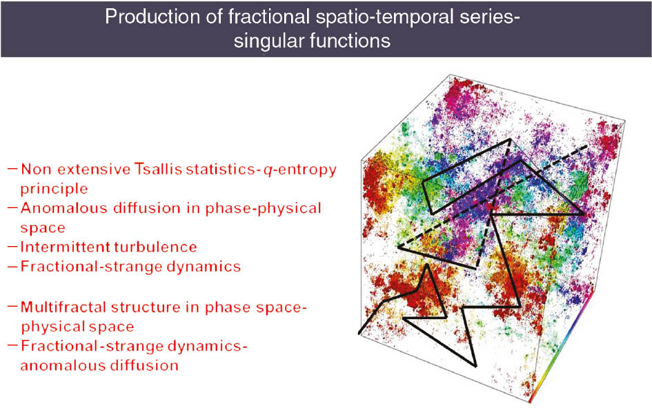
As the dynamics evolves through the multifractal phase space it produce multifractal and singular time series. The phase space is structured as a multifractal set of dynamical microscopical states as the dynamics aims at the Tsallis q-entropy maximaization. In this figure, we have used the Wikipedia multifractal picture in order to show the different regions of phase space corresponding to definite fractal dimension. The black broken line correspond to the the anomalous diffusion and Random Walk of the dynamics in the multifral phase space of the distributed dynamics.
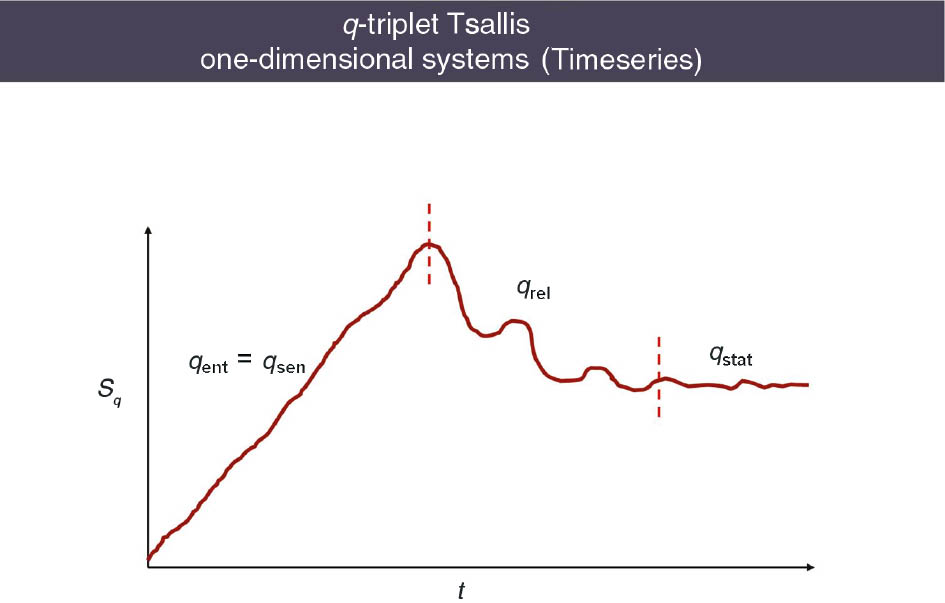
As the dynamics of the system evolves aiming to the q-entropy maximization it produce q-entropy. We can distinguish three different time periods. The first period corresponds to the entropy production through the qsen parameter of the Tsallis q-triplet. The second period corresponds to some kind of relaxation process through the qrel parameter of Tsallis q-triplet. Finally, as the system lives at the stationary state with maximaized q-entropy it reveals fluctuations through the qstat parameter of Tsallis q-triplet.
5.1 The q-triplet of Tsallis
The non-extensive statistical theory is based mathematically on the nonlinear equation:
with solution the q-exponential function defined previously. The solution of this equation can be realized in three distinct ways included in the q-triplet of Tsallis: (qsen, qstat, qrel). These quantities characterize three physical processes which are summarized here, while the q-triplet values characterize the attractor set of the dynamics in the phase space of the dynamics and they can change when the dynamics of the system is attracted to another attractor set of the phase space. The equation (119) for q=1 corresponds to the case of equilibrium Gaussian BG world [2]. In this case of equilibrium BG world the q-triplet of Tsallis is simplified to (qsen=1, qstat=1, qrel=1).
5.1.1 The qstat index and the non-extensive physical states
According to [2] the long range correlated metaequilibrium non-extensive physical process can be described by the nonlinear differential equation:
The solution of this equation corresponds to the probability distribution:
where
for discrete energy states {Ei } by the relation:
for continuous X states {X}, where the values of the magnitude X correspond to the state points of the phase space.
The above distributions functions (122, 123) correspond to the attracting stationary solution of the extended (anomalous) diffusion equation related to the nonlinear dynamics of system. The stationary solutions P(x) describe the probabilistic character of the dynamics on the attractor set of the phase space. The non-equilibrium dynamics can be evolved on distinct attractor sets depending upon the control parameters values, while the qstat exponent can change as the attractor set of the dynamics changes.
5.1.2 The qsen index and the entropy production process
The entropy production process is related to the general profile of the attractor set of the dynamics. The profile of the attractor can be described by its multifractality as well as by its sensitivity to initial conditions. The sensitivity to initial conditions can be described as follows:
where ξ describes the deviation of trajectories in the phase space by the relation: ξ≡limΔ(x)→0{Δx(t)\Δx(0)} and Δx(t) is the distance of neighbouring trajectories. The solution of equation (121) is given by:
The qsen exponent can be also related to the multifractal profile of the attractor set by the relation:
where amin(amax) corresponds to the zero points of the multifractal exponent spectrum f(a). That is f(amin)=f(amax)=0.
The deviations of neighbouring trajectories as well as the multifractal character of the dynamical attractor set in the system phase space are related to the chaotic phenomenon of entropy production according to Kolmogorov-Sinai entropy production theory and the Pesin theorem. The q-entropy production is summarized in the equation:
The entropy production (dS/dt) is identified with Kq, as W are the number of non-overlapping little windows in phase space and N the state points in the windows according to the relation
5.1.3 The qrel index and the relaxation process
The thermodynamical fluctuation – dissipation theory is based on the Einstein original diffusion theory (Brownian motion theory). Diffusion process is the physical mechanism for extremization of entropy. If ΔS denote the deviation of entropy from its equilibrium value S0, then the probability of the proposed fluctuation that may occur is given by:
The Einstein-Smoluchowski theory of Brownian motion was extended to the general FP diffusion theory of non-equilibrium processes. The potential of FP equation may include many metaequilibrium stationary states near or far away from the basic thermodynamical equilibrium state. Macroscopically, the relaxation to the equilibrium stationary state of some dynamical observable O(t) related to the evolution of the system in phase space can be described by the form of general equation as follows:
where Ω(t)≡[O(t)−O(∞)]/[O(0)−O(∞)] is the relaxing relevant quantity of O(t) and describes the relaxation of the macroscopic observable O(t) relaxing towards its stationary state value. The non-extensive generalization of fluctuation – dissipation theory is related to the general correlated anomalous diffusion processes [2]. Now, the equilibrium relaxation process is transformed to the metaequilibrium non-extensive relaxation process:
the solution of this equation is given by:
The autocorrelation function C(t) or the mutual information I(t) can be used as candidate observables Ω(t) for the estimation of qrel. However, in contrast to the linear profile of the correlation function, the mutual information includes the non-linearity of the underlying dynamics and it is proposed as a more faithful index of the relaxation process and the estimation of the Tsallis exponent qrel.
5.2 Measures of multifractal intermittence turbulence
In the following, we follow Arimitsu and Arimitsu [79] for the theoretical estimation of significant quantitative relations which can also be estimated experimentally. The probability singularity distribution P(a) can be estimated as extremizing the Tsallis entropy functional Sq . According to Arimitsu and Arimitsu the extremizing probability density function P(a) is given as a q-exponential function:
where the partition function Zq is given by the relation:
and B(a, b) is the Beta function. The partition function Zq as well as the quantities X and q can be estimated by using the following equations:
We can conclude for the exponent’s spectrum f(a) by using the relation P(a)≈lnd−F(a) as follows:
where a0 corresponds to the q-expectation (mean) value of a through the relation:
while the q-expectation value a0 corresponds to the maximum of the function f(a) as df(a)/da|a0=0. For the Gaussian dynamics (q→1) we have mono-fractal spectrum f(a0)=D0. The mass exponent τ(q̅) can be also estimated by using the inverse Legendre transformation: τ(q̅)=aq̅−f(a) as follows:
where Cq̅=1+2q̅2(1−q)X ln 2.
The relation between a and q can be found by solving the Legendre transformation equation q̅=df(a)/da. Also if we use the equations (135–136) we can obtain the relation:
The q-index is related to the scaling transformations of the multifractal nature of turbulence according to the relation q=1−a. Arimitsu and Arimitsu [79] estimated the q-index by analyzing the fully developed turbulence state in terms of Tsallis statistics as follows:
where a± satisfy the equation f(a±)=0 of the multifractal exponents spectrum f(a). This relation can be used for the estimation of qsen -index included in the Tsallis q-triplet (see next section).
6 Theoretical interpretations of data analysis results
In this section we present more analytically some useful theoretical concents that need for understanding the experimental evidence of complex systems that are presented in part two of this study. These concepts concern the q-CLT and its relation with the q-triplet of Tsallis as well as the fractional dynamics and the anomalous diffusion-random Walk process.
6.1 The q-extension of central limit theorem and the q-triplet of Tsallis
According to the classical central limit theorem, the probability density functions of a sum of independent random variables are Gaussian when the single variables satisfied typical presuppositions. However, the non-Gaussian with heavy tails probability distribution functions, which were observed which are observed in distributed dynamical systems, the statistics of which is related to the q-extension of central limit theorem.
Tsallis non-extensive statistical mechanics includes the q-generalization of the classic CLT as a q-generalization of the Levy-Gnedenko central limit theorem [87] applied for globally correlated random variables. The q-generalization of CLT based at the q-Fourier transform of a q-Gaussian can produce an infinite sequence (qn ) of q-parameters by using the function
For q-Gaussians the q-Fourier transform hold as follows:
where q1=z(q), 1≤q<3.
The q-Fourier transform is defined by Umarov et al. [87] by the formula:
For the inverse q-Fourier transform we have the following formula:
where q−1=z−1(q), 1≤q<3 and
The function z(s) permits the following q-Fourier transform mappings:
as well as the inverse mappings by using the inverse q-Fourier transforms:
We can introduce the sequence qn =zn (q)=z(zn−1(q)), n=1, 2, … starting from the initial q=z0(q), q<3. The qn sequence can be extended for negative integers n=−1, −2, … by q−n =z−n (q)=z−1(z1−n (q)). The sequence qn can be given through the following mappings:
while the duality relations hold:
The q-generalization of the central limit theorem consistent with non-extensive statistical mechanics is as follows:
For a sequence qk, k∈ℤ with qk ∈[1,2] and a sequence x1, x2, xN, … of qk -independent and identically distributed random variable then the zN =x1+x2+xN +… is also a qk−1-normal distribution as N→∞, with corresponding statistical attractor
where q=z(q−1). The q-independence means independence for q=1 and strong correlation for q≠1 [2], [88].
The q-CLT states that an appropriately scaled limit of sums of qk correlated random variables is a qk -Gaussian, which is the
including the triplet (Patt, Pcor, Pscl), where Patt, Pcor and Pscl are parameters of attractor, correlation and scaling rate respectively and corresponds to the q-triplet (qsens, qrel, qstat) according to the relations [87]:
The parameter Patt≡qsens≡qk−1 describes the non-ergodic q-entropy production of the multiscale correlated process as the system shifts to the state of the qatt – Gaussian, where the q-entropy is extremized in accordance with the generalization of the Pesin’s theorem [88]:
The parameter Pcor≡qrel≡qk describes the q-correlated random variables participating to the dynamical process of the q-entropy production and the relaxation process toward the stationary state.
The parameter Pslc≡qstat≡qk+1 describes the scale invariance profile of the stationary state corresponding to the scale invariant q-Gaussian attractor as well as to an anomalous diffusion process mirrored at the variance scaling according to general, asymptotically scaling, form:
Where Px (x) is the probability function of the self-similar statistical attractor G and D is the scaling exponent characterizing the anomalous diffusion process [89]:
The non-Gaussian multi-scale correlation can create the intermittent multi-fractal structure of the phase space mirrored also in the physical space multi-fractal distribution of the turbulent dissipation field. The multi-scale interaction at non-equilibrium critical NESS creates the heavy tail and power law probability distribution function obeying the q-entropy principle. The singularity spectrum of a critical NESS corresponds to extremized Tsallis q-entropy.
In this framework of theoretical modeling of distributed random fields, the fractal-multifractal character of the distributed dynamical systems at every NESS (week or strong turbulence) as it was shown in this study, indicate the existence of physical local singularities for the spatial-temporal distribution of distributed physical variables. The singularity behavior of a given random field function f(x) at a given point x* is defined as the greatest exponent h so that f is Lipschitz h at x* [67]. The Hölder exponent h(x*) measures how irregular f is at the point X* according to the relation:
Where Pn (x) is a polynomial vorter n. If h(x*)∈(n, n+1) then f(x) is n-times but not n+1 times differentiable at the point x*. The smaller the exponent h(x*) is the more irregular (singular) is the function f at the point x*. On a self similar fractal set the singularity strength of the measure μ at the point x is described by the scaling relation:
Where Bx (ε) is a ball of size (ε) centered at x and μ(Bx ) is the fractal mass in the Bx region. Homogeneous measures are characterized by a singularity spectrum supported by a single point (a0, f(a0)) while multifractal sets involve singularities of different strengths (a) described by the singularity spectrum f(a).
The singularity spectrum is defined as the Hausdorff dimension of the set of all points x such that a(x)=a. The singularity strength a(x) of the fractal mass measure is related to the local fractal dimension D of the fractal set. More generally, the singularity spectrum associated with singularities h (Hölder exponents) of a distributed random variable is given follows:
That is D(h) is the Hausdorff dimension of the set of all points x such as h(x)=h. For the case of space plasmas or fluids the singularity spectrum D(h) corresponds to the scaling invariance of the MHD description according to the scaling transformation of the MHD equations:
where h is a free parameter and ur, br are the velocity and magnetic fields of the solar wind plasma system, correspondingly [90]. The a(x) singularity exponent of the fractal mass measure and the f(a) singularity spectrum describes the scaling of the energy dissipation in the solar wind turbulent system.
The fractal-multifractal structure of the general dynamical systems (particles and fields) indicates the generalization of the classical field-particle dynamics to the fractional dynamics, since the functions of the distributed physical system’s variables are irregular and they are produced by fractional dynamics on fractal structures. The differentiable nature of smooth distribution of the macroscopic picture of physical processes is a natural consequence of the Gaussian microscopic randomness which, through the classical CLT, is transformed to the macroscopic, smooth and differentiable processes. The classical CLT is related to the condition of time-scale separation, where at the long-time limit the memory of the microscopic non-differentiable character is lost. On the other hand, the q-extension of CLT induces the nonexistence of time-scale separation between microscopic and macroscopic scales as the result of multiscale global correlations which produce fractional dynamics and singular functions of spatio-temporal dynamical physical variables.
6.2 Fractional calculus
Far from equilibrium, the dynamics of distributed systems produces fracat-multifractal structure. For this, we must extend the smooth mathematical description of the system with fractional description by using fractional derivatives and integrals. Fractal sets are measurable metric sets with non-integer Hausdorff dimension. The elements of a fractal set can be represented by n-tuples of real numbers x=(x1, x2, …, xn ) such that a fractal set F is embedded in Rn . A fractal function is defined on a fractal set as follows according to Tarasov [91]:
where XE is the characteristic function of E. The continuous function f(x) is defined as follows:
where
The Lebesque – Stieltjes integral over a D-dimensional fractal set of a function f(x) is defined by:
and it can be proved to be given by the relation:
where
The nonlocal character is evident in both cases of fractional derivative and integral on a fractal set. The nonlocal character of fractional calculus is related to multiscale and self-similar character of the fractal structure. The fractional extension of integral and differential calculus can be used for the description of the non-local multiscale phenomena described by fractional equations as the fractional laws of materials, or fractional field equations in fluids, or other distributed systems. Also the Lagevin or the Fokker-Planck equation are transformed to fractional equations [25], [26], [41], [91]. The solution of the fractional equations correspond to fractional non-differentiable singular self-similar functions as we can observe at the experimental data.
Milovanov and Zelenyi [93] introduced the fractional wave equation for the description of space plasma or other distributed systems where fractons excitations, namely fractional waves on fractals can be excistense. The fractional extension of wave equations for spherically symmetric vibrations of fractals includes temporal and spatial fractional derivatives as follows:
where
is the fractional time derivative, D is the fractal dimension of space and θ is the connectivity index of the fractal space. The nonlocal character of the fractional wave equation on fractals is related to the correlated and coherent character of local dynamical events on a self-similar structure. The solution of the fractional wave equations contains exponentially decaying factors which are absent in Euclidian solutions. These factors are responsible for the spatial localization of fractons, while the strength of localization is described by the connectivity index θ, through the localization exponent 2+θ/2, which coincides with the Hausdorff dimension of the “geodesic lines” on the fractal space. The localization of waves on fractals (fractons) can be used for the explanation of local variation of solar wind characteristics, especially during shock events.
6.3 Anomalous diffusion and strange dynamics
Nonlinear dynamics can create fractal structuring of the phase space and global correlations in the nonlinear system. For nonextensive systems the entire phase space is dynamically not entirely occupied (the system is not ergodic), but only a scale-free –like part of it is visited yielding a long-standing (multi)-fractal-like occupation. According to Milovanov and Zelenyi [69], Tsallis entropy can be rigorously obtained as the solution of a nonlinear functional equation referred to the spatial entropies of the subsystems involved including two principal parts. The first part is linear (additive) and leads to the extensive Boltzman-Gibbs entropy. The second part is multiplicative corresponding to the nonextensive Tsallis entropy referred to the long range correlations. The fractal –multifractal structuring of the phase space makes the effective number Weff of possible states, namely those whose probability is nonzero, to be smaller (Weff<W) than the total number of states.
According to Zaslavsky [24] the topological structure of phase space of nonlinear dynamics can be highly complicated including trapping and flights of the dynamics through a self-similar structure of islands. The island boundary is sticky making the dynamics to be locally trapped and “stickiness”. The set of islands is enclosed within the infinite fractal set of cantori causing the complementary features of trapping and flight being the essence of strange kinetics and anomalous diffusion.
The dynamics in the topologically anomalous phase space corresponds to a random walk process which is scale invariant in spatial and temporal self-similarity transform:
The spatial-temporal scale invariance causes strong spatial and temporal correlations mirrored in singular self-similar temporal and spatial distribution functions which satisfy the fractional generalization of classical Fokker-Planck-Kolmogorov equation (fFPK equation) [24]:
where P≡P(ξ, t) is the probability density of the state (ξ) at the time (t).
The critical components (a, β) correspond to the fractal dimension of spatiotemporal nongaussian distribution of the temporal-spatial functions-processes or probability distributions. The quantities A, B are given by:
where <<…>> denotes a generalized convolution operator [94].
The FFPK equation is an archetype fractional equation of fractional stochastic dynamics in a (multi)-fractal phase space with fractal temporal evolution caused by the self similar and multiscale structure of islands around islands, responsible for the flights and trappins of the dynamics. The “spatial” random variable can be any physical variable, such as position in physical space, velocity in the velocity space or a dynamic field (magnetic or electric) at a certain position in physical space, stresses in materials etc, underlying to the nonlinear chaotic dynamics. The fractional dynamics of plasma includes fractal distribution of field and currents, as well as fractal distribution of energy dissipation field.
The fractional temporal derivative ∂β /∂tβ in kinetic equations allows one to take fractal-time random walks into account, as the temporal component of the strange dynamics in fractal-turbulent media. The waiting times follow the power law distribution P(τ)~τ−(1+β) since the “Levy flights” of the dynamics also follow the power law of distribution.
The asymptotics (root mean square of the displacement) of the transport process is given by
The solution of the fractional kinetic equation corresponds to Levy distributions and asymptotically to Tsallis q-Gaussians. According to Alemany and Zanette [95], the set of points visited by the random walker can reveal a self-similar fractal structure produced by the extremization of Tsallis q-entropy. The q-Gaussian distribution of the fractal structure created by the strange dynamics and the extremized q-entropy asymptotically corresponds to the Levy distribution P(ξ)~ξ−1−γ where the q-exponent is related to the Levy exponent γ by
The well-known Boltzmann’s formula S=k log W where S is the entropy of the system and W is the number of the microscopic states corresponding to a macroscopic state indicates the priority of statistics over dynamics. However, Einstein preferred to put dynamics in priority of statistics, using the inverse relation i.e. W=eS/k where entropy is not a statistical but a dynamical magnitude. Already, Boltzmann himself was using the relation
where the variables x corresponds to physical distributed variables of the system, while P(x, t) describes the probability distribution of the particle-fields variables.
The variables A(x), B(x) corresponds to the first and second moments of probability transfer and describe the wandering process in the fractal space (phase space) and time. The fractional space and time derivatives ∂β /∂tβ, ∂α /∂xα are caused by the multifractal (strange) topology of phase space which can be mirrored in the spatial multifractal distribution of the dynamical variables.
The q-statistics of Tsallis corresponds to the meta-equilibrium solutions of the fFPK equation [26], [97]. Also, the metaequilibrium states of fFPK equation correspond to the fixed points of Chang non-equilibrium RGT theory for space plasmas [24], [98]. The anomalous topology of phase space dynamics includes inherently the statistics as a consequence of its multiscale and multifractal character. From this point of view the non-extensive character of thermodynamics constitute a kind of unification between statistics and dynamics. From a wider point of view the fFPK equation is a partial manifestation of a general fractal extension of dynamics. According to Tarasov [25], the Zaslavsky’s equation can be derived from a fractional generalization of the Liouville and BBGKI equations. According also to Tarasov [25], [26], [41], the fractal extension of dynamics including the dynamics of particles or fields is based on the fact that the fractal structure of matter (particles, fluids, fields) can be replaced by a fractional continuous model. In this generalization, the fractional integrals can be considered as approximations of integrals on fractals. Also, the fractional derivatives are related with the development of long range correlations and localized fractal structures.
6.4 Fractal topology, critical percolation and stochastic dynamics
The nonlinearity in the dynamics of the solar wind plasma system including fields (B, E) and particles can create random distributions in space of dynamical fields and material fields (bulk, velocity, pressure, temperature, fluxes, currents etc). In this section we follow Milovanov and Zimbardo [99] and Milovanov [9] and present some basic concepts concerning topological aspects of percolating random fields.
For any random field distribution ψ(x) in the n-dimensional space (En ) there exists a critical percolation threshold which divides the space En into two topological distinct parts: Regions where ψ(x)<hc marked as “empty”, and regions where ψ(x)>hc, marked as “filled”. When ψ(x)≠hc, one of these parts will include an infinite connected set which is said to percolate. As the threshold h changes we can find the critical threshold hc where the topological phase transition occurs, namely the nonpercolating part starts to percolate.
The geometry of the percolating set at the critical state (h→hc ) is a typical fractal set for length scales between microscopic distances and percolation correlation length which diverges. The statistically self-similar geometry includes power-law behavior of the “mass” density of the fractal set such as “fractal mass density” ~xD–n, where x is the length scale, D is the Hausdorff fractal dimension which must be smaller than the dimensionality (n) of the embedding Euclidean space. In addition to the parameter D of the fractal dimension, there is the index of connectivity θ which describes the “shape” of the fractal set and may be different for fractals even with equal values of the fractal dimension D. The index of connectivity θ is defined as characterizing the shortest (geodesic) line connecting two different points on the fractal set by the relation dθ =(2+θ)/2, where dθ is the minimal Hausdorff dimension of the minimal (geodesic) line. The geodesic line on a self-similar fractal set (F) is a self affine fractal curve whose own Hausdorff fractal dimension is equal to (2+θ)/2. The index of connectivity plays an essential role in many dynamical phenomena on fractals, while it is a topological invariant of the fractal set F.
From the fractal dimension D and the connectivity index θ we can define a hybrid parameter ds =2D/2+θ which is known as the spectral or the fracton dimension which represents the density of states for vibrational excitations in fractal network termed as fractions [9]. The root mean square displacement of the random walker on the fractal set is given by:
Where dθ is the fractal dimension of the self-affine trajectory on the fractal set. Also, the spectral dimension which measures the probability of the random walker to return to the origin, is given by:
while the Hausdorff fractal dimension D is a structural characteristic of the fractal structure F, the spectral dimension ds mirrors the dynamical properties such as wave excitation, diffusion etc. The fractal dimension D of the fractal structure F of a percolating random field distributed in the En Euclidian space is given by D=n–β/ν, where β, ν are the universal critical exponents of the critical percolation state [9]. According to the Alexander-Orbach (AO) conjecture [100], the spectral dimension ds has been established to be equal to the value ds =4/3, for all embedding dimensions n≥2. Especially, for embedding dimensions 2≤n≤5, Milovanov [100] has improved the AO conjecture to the value ds =c≃1327, where c is the percolation constant. This constant determines the minimal fractional number of the degrees of freedom that the random walker must have to reach the infinitely remote point in the Euclidian embedding space En . According to Milovanov [9], [100], [101] and Milovanov and Zelenyi [69] the fractal topology and critical percolation theory transform the description of plasma diffusion, bulk flow and electrodynamical-MHD phenomena from classical smooth equations to fractional equations description.
The diffusion coefficient is now expressed in terms of the connectivity index θ=(μ–β)/ν and the Hausdorff dimension of the infinite percolation cluster df =n–β/ν where β, μ, ν are the universal critical percolation parameters. The Maxwell equations for the plasma current system are transformed to fractional equations including fractional derivatives of the magnetic field given by:
where s, w are spatial variables.
The fractional extension of Maxwell equations is caused by the non-local self-similar hierarchical structuring of the plasma system, while the degree of non-locality is quantified by the connectivity index included in the power exponent γ=2/(2+β) in the singular kernel (s−w)−γ . The interaction of plasma charged particles and dynamical fields described by fractional Maxwell equations and fractional transport equations causes self-consistency in the fractal distribution of dynamical (magnetic-electric) fields, of bulk plasma flow fields and energy dissipation fields. In this way, the fractal dimension and connectivity index (θ) of dynamical field’s distribution is self-consistently related to the fractal dimension (D+) and the index of connectivity (θ+) of material fields.
6.5 Renormalization Group (RNG) theory and phase space transition
The multifractal and multiscale intermittent turbulent character of the distributed dynamics can be verified after the estimation of the spectrum f(a) of the point wise dimensions or singularities (a). This justifies the application of RG theory for the description of the scale invariance and the development of long-range correlation of the distributed systems and intermittent turbulence state. Generally the non-equilibrium distributed random dynamics can be described by generalized Langevin stochastic equations of the general type:
where fi corresponds to the deterministic process as concerns the plasma dynamical variables ϕ(x, t) and ni to the stochastic components (fluctuations). Generally, fi are nonrandom forces corresponding to the functional derivative of the free energy functional of the system. According to Chang [38], [102] the behavior of a nonlinear stochastic system far from equilibrium can be described by the probability density functional P, defined by:
where
Moreover, the far from equilibrium renormalization group theory applied to the stochastic Lagrangian L generates the singular points (fixed points) in the affine space of the stochastic distributed system. At fixed points the system reveals the character of criticality, as near criticality the correlations among the fluctuations of the random dynamic field are extremely long-ranged and there exist many correlation scales. Also, close to dynamic criticality certain linear combinations of the parameters, characterizing the stochastic Lagrangian of the system, correlate with each other in the form of power laws and the stochastic system can be described by a small number of relevant parameters characterizing the truncated system of equations with low or high dimensionality. This is the nonequilibrium RG theory explanations of self-organization process and dynamical reduction of degrees of freedom. According to these theoretical results, the stochastic system can exhibit low dimensional chaotic or high dimensional SOC like behavior, including fractal or multifractal structures with power law profiles. The power laws are connected to the near criticality phase transition process which creates spatial and temporal correlations as well as strong or weak reduction (self-organization) of the infinite dimensionality corresponding to a spatially distributed system. Critical phase transition processes can be related to discrete fixed points in the affine dynamical (Lagrangian) space of the stochastic dynamics. The SOC or chaos like behavior of distributed dynamics corresponds to the second phase transition process as the system lives at different fixed points of RG. The probabilistic solution (173) of the generalized Langevin equations may include Gaussian or non-Gaussian processes as well as normal or anomalous diffusion processes depending upon the critical state of the system.
From this point of view, a SOC or low dimensional chaos interpretation or distinct q-statistical states with different values of the Tsallis q-triplet depends upon the type of the critical fixed (singular) point in the functional solution space of the system. When the stochastic system is externally driven or perturbed, it can be moved from a particular state of criticality to another characterized by a different fixed point and different dimensionality or scaling laws. Thus, the old SOC theory could be a special kind of critical dynamics of an externally driven stochastic system. After all SOC and low dimensional chaos can coexist in the same dynamical system as a process manifested by different kinds of fixed (critical) points in its solution space. Due to this fact, the distrtibuted dynamics may include high dimensional SOC process or low dimensional chaos or other more general dynamical process corresponding to various q-statistical states. The non-extensive character of the distributed dynamics related with q-statistical metaequilibrium thermodynamics as well as the existence of long-range correlations must be harmonized with the nonlinear dynamics of the distributed system as well as the non-equilibrium extension of RGT. This is the base for the development of anomalous diffusion plasma processes, long-range correlations and scale invariance which can be amplified as the system approaches far from equilibrium dynamical critical points. Also, it is known that nonlinear dissipative dynamics with finite or infinite degrees of freedom includes the possibility of self-organizing reduction of the effective degrees of freedom and bifurcation to periodic or strange (chaotic) attractors with spontaneous development of macroscopic ordered spatiotemporal patterns.
The bifurcation points of the nonlinear dynamics, corresponds to the critical points of far from equilibrium non-classical statistical mechanics and its generalizations, as well as to the fixed points of the RGT. The RGT is based in the general principle of scale invariance of the physical processes as we pass from the microscopic statistical continuum limit to the macroscopic thermodynamic limit. For introducing the mechanism of the RGT at distributed dynamics we start with the generalized Langevin equation:
Where F is the free energy of the system and Γ is the relaxation rate and N is the noise component with the correlation:
corresponding to the distributed physical magnitude of the solar wind plasma system. The structure of these equations (174, 175) can be produced by using the BBGKY (Bogoliubov-Born-Green-Kirkood-Yvon) hierarchy included in the Liouville equation applied at the stochastic system particles and fields. Also, the structure of Langevin equation ensures that the metaequilibrium distribution is always attained as t→∞. In the following and according to Tsallis q thermodynamic theory we conjecture in relation with Langevin equations the generalization of the Free energy functional to the q-Free energy functional Fq so that the Langevin equation can be related to a q-generalized Fokker-Planck equation of. By using the q-generalized Fokker – Planck equation we can estimate the N-point correlation function (GN ) of the plasma system, as well as, the partition function Zq as the functional integrations:
The N-point q-correlation function is related to the functional derivative of partition function as follows:
For the estimation of the system’s partition function it makes no sense to consider fields, which varies rapidly on scales shorter than a characteristic microscopic dimension and such field should be excluded from the estimation of the partition function, as well as, from the application of scale transformation according to the RGT. This can be succeeded by a suitable cutoff parameter of the Fourier transform of the distributed plasma properties. According to Wilson [19] and Chang [38] the dynamics of distributed system as it approaches the critical points includes a cooperation of all the scales from the microscopic to macroscopic level. The multiscale and holistic distributed dynamics can be produced by scale invariance principle included in the RG transformation corresponding to the flow:
where
At the fixed points
implies that the correlation length at the fixed point must be either zero or infinite. Also, as the zero value is without physical interest we conclude the infinite correlation of the system at the fixed point
7 Summary and discussion
Figure 4 presents the most significant concepts and theoretical characteristics of the dynamics and statistics as the distributed dynamical system departs from the thermodynamic equilibrium and lives at metaequiilibrium states with exramized q-entropy. At the thermodynamic equilibrium state the system reveals weak complex character while far from equilibrium the full complex character is manifastated. Near thermodynamic equilibrium statistics and dynamics are two separated but fundamental elements of the physical theory. Also, at thermodynamical equilibrium, nature reveals itself as a Gaussian and macroscopically uncorrelated process simultaneously with unavoidable or inevitable and objective deterministic character. However, modern evolution of the scientific knowledge reveals the equilibrium characteristics of the physical theory as an approximation or the limit of a more synthetic physical theory, which is characterized as complexity. The new physical characteristics of complexity theory can be manifested as a physical system is driven in far from equilibrium states.
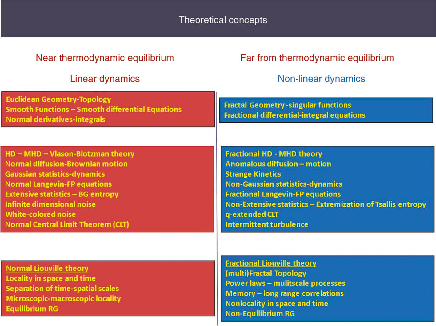
In this table we summarize the q-extension of dynamics and statistics as the system departs from the state of thermodynamic equilibrium and lives at meta equilibrium stationary states.
Moreover, far from equilibrium statistics and dynamics can be unified through the Tsallis nonextensive statistics included in Tsallis q-entropy theory [2] and the fractal generalization of dynamics included in theories developed by Ord [76], Nottale [13], Castro [12], Zaslavsky [24], Shlesinger et al. [7], Kroger [60], Tarasov [25], [26], [41], El-Nabulsi [29], [61], Cresson and Greff [40], Goldfain [30], [84] and others. Also, the new non-extensive characteristics of non-equilibrium physical theory for distributed physical systems were verified experimentally until now by Pavlos [64], [86], [103], [104], Iliopoulos et al. [105] and Karakatsanis and Pavlos [106], [107] in many cases.
Generally, the traditional scientific point of view is the priority of dynamics over statistics. That is dynamics creates statistics. However, for a complex system the holistic behaviour does not permit easily such a simplification or division of dynamics and statistics. From this point of view Tsallis statistics and fractal or strange kinetics are two faces of the same complex and holistic (non-reductionist) reality. As Tsallis statistics is an extension of Boltzmann-Gibbs statistics, we can support that the thermal and the dynamical character of a complex system are the manifestation of the same physical process which creates extremized thermal states (extremization of Tsallis entropy) or extremized mechanical actions, as well as dynamically ordered states. From this point of view the Feynman path integral formulation of the statistical physical theory and of the quantum probabilistic theory indicates the indivisible thermal and dynamical character of physical reality [31]. After Heisenberg’s revolutionary substitution of physical magnitudes by operators and the following probabilistic interpretation of Heisenberg operationalistic concepts and Schrodinger wave functions done by Max Born [54], probability obtained clearly a new realistic and ontological character concerning the foundation of physics [108]. Moreover, the development of complexity theory caused the extension of the probabilistic character of dynamics from microscopic (quantum theory) to macroscopic (classical theory) level of reality. This showed the deeper meaning of the Boltzmann entropy principle through the fractal extension of dynamics, as well as the q-extension of statistics according to Tsallis non-extensive entropy theory.
Prigogine [34] and Nicolis [49] were the principal leaders of an outstanding transition to the new epistemological ideas from microscopic to the macroscopic level, as they discovered the admirable self Self-Organization operation of the physical-chemical systems. That is, the possibility for the development of long-range spatiotemporal correlations, as the system lives far from equilibrium. Thus, Prigogine and Nicolis opened a new road towards the physical understanding of random fields and statistics, related to the non-Gaussian character of the physical processes. This behaviour of nature is known as non-equilibrium development of dissipative structrures or self-organization process. Prigogine’s, Haken’s and Nicoli’s self-organization concepts inspired us to introduce the self organization theory as a basic tool for the description of many complex systems. In this direction the dynamics of the space plasmas [86], [104], [109], seismogenesis [105], as well as the dynamics of brain activity [110] has been decribed as a non-equilibrium and self-organization process. Parallely to the scientific work of Brussels’ school, Lorenz [111] discovered the Lorenz’s attractor as the weather’s self organization process, while other scientists had already observed the self organization process in the dynamics of fluids (e.g. dripping faucet model) or elsewhere, verifying the Feigenbaum [112] mathematical scenarios to complexity included in nonlinear maps or Ordinary Differential Equations-Partial Differential Equations [113]. However, although there was such a wide development of complexity science, scientists till now prefers to follow the classical theory, namely that macro-cosmos is just the result of fundamental laws which can be traced only at the microscopical level. Therefore, while the classical reductionistic theory considers the chaotic and the self-organization macroscopic processes as the result of the fundamental Lagrangian or the fundamental Hamiltonian of nature, there is an ongoing different perception. Namely, that macroscopic chaos and complexity cannot be explained by the hypothetical reductionistic point of view based at the microscopic simplicity, but they are present also in the microscopic level of physical reality.
Therefore, scientists like Nelson [114], Hooft [5], Parisi [37], Beck [3] and others, used the self-organization concept process of the complexity science for the explanation of the microscopic “simplicity”, introducing theories like stochastic quantum field theory or chaotic field theory. This new perception started to appear already through the Wilson’s theories of renormalization, which showed the multiscale cooperation in the physical reality [19]. At the same time, the multi-scale dynamical cooperation produces the self-similar and the fractal character of nature allowing the application of renormalization methods at non-equilibrium critical states of physical systems. This leads to the utilization of fractal geometry into the extended unification of physical theories, since the fractal geometry includes properties of stochastic multiscale and self-similar character. Scientists like Ord [76], El Naschie [27], Nottale [13] and others, introduced the idea of fractality into the geometry of space-time itself negating the notion of differentiability of physical variables. Also the fractional geometry is connected to non-commutative geometry since for fractional objects the principle of self similarity negates the Eycleidian notion of the simple geometrical point (as that which has no-parts), just like it negates the idea of differentiability and determinism.
Therefore, the fractional geometry of space-time leads to the fractal extension of dynamics exploiting the fractal calculus (fractal integrals-fractal derivatives) [25], [26], [30], [40], [41], [48]. Also, the fractal structure of space-time includes intrinsically a stochastic character as the presupposition for determinism is differentiability [13], [40]. In this way, statistics is unified with dynamics automatically, while the notion of probability obtains a physical substance, characterized as dynamical probabilism. The ontological character of probabilism can be the base for the scientific interpretation of self-organization and ordering principles just as Prigogine [34] had imagined, following the Heisenberg’s concept. From this point of view, we could say that contemporary physical theory returns to the Aristotle’s potentiality point of view, as Aristotelianism’s potentiality theory includes the Newton’s and Democritus’ mechanistical determinism only as one component among others in the organism-like behaviour of Nature [115]. Modern evolution of physical theory, as it was described previously, is highlighted in Tsallis q-generalization of the Boltzmann-Gibbs (B-G) statistics which includes the classical (Gaussian) statistics, as the q=1 limit of thermodynamical equilibrium. Far from equilibrium, the statistics of the dynamics follows the q-Gaussian generalization of the B-G statistics or other more generalized statistics. At the same time, Tsallis q-extension of statistics is related to the fractal generalization of dynamics. However, for complex systems, their holistic behaviour does not easily permit such a simplification and division of dynamics and statistics. The Tsallis extension of statistics and the fractal extension of dynamics as strange kinetics are two faces of the same complex and holistic (non-reductionist) reality. Moreover, the Tsallis statistical theory including the Tsallis extension of entropy, known as q-entropy principle, [2] the fractional generalization of dynamics [7], [24] as well as the scale relativity extension of the Ainstein Relativity theory, parallely to the scale extension of relativity theory [12], [13] are the cornerstones of modern physical theory related to non-linearity and non-integrability as well as to the non-equilibrium ordering and the self organization principle of nature.
In the following, we summarized and discussed the highlights of complexity theory as the road of the global unification of the physical theory from microscopic to macroscopic level of physical reality.
7.1 The Thermodynamics point of view
Complexity theory becomes effective when dynamical system exists far from equilibrium, where the entropy follows the equation:
Far from equilibrium, according to Tsallis theory, the Boltzmann-Gibbs entropy:
is the limit of a more general and non-extensive entropy. The non-extensive Tsallis entropy Sq given by the equation:
For q=1 the new and non-extensive statistical mechanics is transformed to the known Boltzmann-Gibbs statistical mechanics [2].
Every thermodynamical system is also a dynamical system with internal dynamical states and this point of view exists as the propabilistic character of the internal dynamics. Thus, the entropy corresponds to the information that can be obtained by knowing the internal microscopic state of the system.
Near equilibrium δS=0 and δ2S is a Lyapunov function of positive time derivative. The time derivative corresponds to entropy productions.
However far from equilibrium the time derivative of δ2S is may be negative corresponding to decreasing of entropy and development of order [2]. Significant concepts of Thermodynamics developed for the near equilibrium phenomena can be used for the description of far from equilibrium phenomena. Such concepts are: thermodynamical potentials, phase-transition, order parameters, nucleation phenomena. Also the Ginzburg-Landau theory can be extended for the description of the far from equilibrium phase transition processes and pattern formation in many different dynamical systems [31].
7.2 The dynamical point of view
Complex systems can be at the same time thermodynamical and dynamical systems. The far from equilibrium dynamics can be described by the generalized free energy H function which depends generally upon the macroscopic field
where f is stochastic noise.
The Langevin equation (184) is equivalent to a functional Fokker-Planck equation:
where
The probability density functional can be calculated by the method of math integral formalism. According to Chang [102], for nonlinear stochastic systems near criticality the correlations among the fluctuations of the random dynamical fields are extremely long-ranged and there exist many correlations states. The far from equilibrium generalization of the renormalization group transformation includes the existence of fixed points (singular point) for the Lagrangian scaling flow on the parameter stochastic Lagrangian affine space. As the stochastic nonlinear-complex system is perturbed from a particular fixed point (meta-equilibrium state) it may be attached to another critical state revealing symmetry breaking and phase transition processes.
Anomalous diffusion and non-Gaussian distributions, low dimensional chaos, self organized critically, spatiotemporal chaos, spatiotemporal patterns, directed percolation processes, scaling and other macroscopic complex phenomena can be described by the application of the generalized renormalization group theory. In the above description the Langevin equations can be of more general type corresponding to a general type of master equations and discrete spatio-temporal stochastic or deterministic chaotic processes. According to the relation:
where |Pt 〉 is the probability distribution vector and L the so-called Liouville operator which generates the temporal evolution [116]. It is a truth that from the microscopic to the macroscopic level, the modern physical theory includes non-linear dynamical processes in finite-dimensional or infinite-dimensional state spaces. The dynamical processes can be of different and independent form at every level of dynamical description of nature. Superstrings, elementary particles or other physical forms and patterns observed at the macroscopic or cosmological level can be produced as solutions of non-linear mathematical equations including Hamiltonians, Lagrangians, and other mathematical forms corresponding to continuing or discrete fields, quantum or classical.
The great dream of theoretical scientists is to develop some kind of organizing physical principles valid at all levels. The strong simultaneous presence of chaos and fractal self-similarity at the macroscopic and at the quantum level indicates the possibility for the existence of such global organizing principles. Some significant concepts in this direction are described in the following.
7.3 Fractal theory space and renormalization group theory
According to Nottale [13] theory space can be endowed with certain geometrical symmetries based essentially on the renormalization group (RG) transformations. Fractal lattices, known already in condensed matter physics, are used to construct classes of new theory spaces. Theory space lattices are defined recursively by replacing each site with a new simplex of S sites, while this process is iterated k times.
In the limit K→∞ this lattice describes a continuum theory whose properties are determined be certain scaling laws of critical systems. At finite critical temperature the Feynman path integral is invariant under the RG transformations. Wilson’s approach is based on an effective action
where ZA is the partition function and the integration extends over a functional space of fields.
According to Morozov and Niemi [117], a RG flow could indeed tend towards a nontrivial attractor with even a fractal structure corresponding to a chaotic flow in the space of couplings. This could lead to a Big Mess scenario in applications to multiphase systems, from spin-glasses and neural networks to fundamentals string theories. The concept of the fractal theory space can be extended in a general unifying scheme to include Langevin processes or directed percolation processes corresponding to macroscopic far from equilibrium processes [118], [119], [120].
7.4 Scale relativity theory
According to Nottale [121], [122], [123] the Scale Relativity theory extends the Einstein Relativity theory to scale transformations of resolution [25], [48]. In this theory the axiom of space-time differentiability is given up and the space-time corresponds to a fractal set. This is in accordance with Feynman’s path integral approach to quantum mechanics, which at small length and time scales reveals continuous and non-differentiable paths with fractal dimension D=2. The fractal character of space-time indicates that the space-time variables can be described as depending also on resolutions Φ=φ(x, ε). Nottale extended the principle of Relativity theory to scale Relativity, which the laws of nature should apply to all reference systems whatever their state if scale. This is a scale covariance principle in the spirit of renormalization group theory corresponding to the typical form:
In this theory the probabilistic character of quantum theory is derived naturally by the fractal nature of space-time while the microscopic quantum laws and the macroscopic stochastic processes are the different manifestation of the same physical law under the scale transformation in the fractal space-time. This led us to consider the macroscopical chaos and complexity in natural systems as the manifestation of the large scale fractal nature of space-time. From this point of view, the Feynman path integral formulation of physical theory in a fractal space-time is the unifying tool of the microscopic and macroscopic complexity. In this way, the path probability density, the correlation function and the generating functional are the common tools in a unified point of view of microscopic and macroscopic stochastic processes according to the relation:
where, ZG =∫Dφe−H(J) is the partition function of the system and GN the correlation functions.
Classical macroscopic distributed far from equilibrium systems and microscopic quantum field systems are connected through stochastic and chaotic quantization theory. According to the Parisi and Wu [124] approach the classical field Φ described by an action S[φ] can be quantized by means of a stochastic Langevin equation:
where f denotes spatio-temporal Gaussian white noise.
The classical stochastic process corresponds to a non-equilibrium D+1 dimensional space-time system while its corresponding Fokker-Planck distributed equation at the equilibrium state is identified with the theory of the quantum field Φ in the D-dimensional space-time. The classical stochastic dynamics in the D+1 dimensional space-time is described by the correlators 〈Φ(x1, t1), Φ(x2, t2), …., Φ(xn, tn )〉, where Φ(x, t) are the solutions of equation (190). The classical stochastic correlators in the limit t→∞ reproduce the Feynman graphs of the corresponding D dimensional quantum theory.
On the other hand, according to Beck [3], [125] there are deterministic chaotic dynamical systems that can generate the Langevin dynamics of equation (184). This approach corresponds to the chaotic quantization theory as it simulates quantum fields by chaotic dynamics. Moreover, Beck introduced a class of coupled map lattices, by using coupled third – order Tschebyscheff polynomials, which can simulate quantum field theories. The stochastic and chaotic quantization theories reveal the mathematical similarity of the classical and quantum dynamics but more than this it indicates the deep unity of physical theory at the microscopic and the macroscopic level. This point of view can be supported by modern theoretical constructions, which can produce the quantum theory as the manifestation of a subquantum chaotic dynamics.
Hooft [5], [6] conjectured that quantum mechanics can logically arise as the low energy limit of a microscopically deterministic but dissipative theory. Biro et al. [4] showed that quantum field theory can emerge in the infrared limit of a high-dimensional quantum field theory as Yang- Mills fields can quantize themselves.
7.5 Becoming before being
Quantum theory and Relativity theory (special and general) introduced the notion of becoming in the heart of being showing that being is the production of becoming. Complexity theory is a theory of being as Becoming in its essence. From this point of view we believe that complexity theory, as the essential theory of becoming and pattern formation, shows the route for a global unification of physical theory. Particularly, the quantum states include becoming and potentiality in an objective way. Because of this the physical magnitudes are related probabilistically with the quantum states. Entropy and complexity are inherent in the quantum states. Similarly, in relativity material particles are condensed energy and space and time are continuously. In this point of view the great Hellenic philosophers Heraclitus, Plato and Aristotle meet one another. For Heraclitus all the cosmos is one. For Aristotle matter is the potentiality of the being and for Plato the essence of things is the form.
According to the modern theoretical concepts, the essence of the physical theory is the mathematical structure-equations with solutions corresponding to the observed phenomena. All this state of knowledge can be included in the general form of Feynman path integral formulation of the probability amplitudes of dynamics:
where Φ is the dynamical state and S the action functional of the dynamics.
The unification of micro and macro dynamics passes through the fractal theory, and the scale invariance of Feynman amplitudes. The Feynman principle must be related somehow to the general probabilistic Liouville dynamical theory. As we show in the following, the probabilistic character of modern theory reveals the fundamental character of becoming or process in the physical theory. According to the radical conjecture of Prigogine becoming is prior to being in a fundamental way including even the physical laws. According to Kovacs [51] many of the pattern formation processes observed in systems of quite different genesis exhibit astonishing analogies independently of the composition of the system and of the interactions between individual components. As the formation of structures is a geometrical event, the observed qualitative analogies indicate common topological origin. From this point of view, physics is geometry and topology.
In this direction bifurcation theory and symmetry breaking processes are the common base of the far from equilibrium dynamics in micro and macro cosmos. In the bifurcation theory, bifurcation phenomena include topological equivalence while the bifurcations are largely determined by geometrical constraints as the dimension and shape or inherent symmetries. The structural stability of physical patterns at every level of physical reality is inherent in the fundamental law (laws) of physics derived by geometrical invariance principles such as space-time symmetries or gauge symmetries. The link between geometry and physics is due to topological invariance principles which cause inherent stability properties. Structural stability proves includes the interaction and correlation physical phenomenology of physical systems. On the other hand, self-organization is a far from equilibrium thermodynamical process revealing entropy decrease and order development according to the equation:
where deS is the reversible entropy transfer and diS is the irreversible producedentropy within the system.
Thermodynamics is coupled to dynamic through the general Liouville equation:
where f(t) is the infinite dimensional distribution vector f(t)={f0, f1(x1), f2(x1, x2), ….}, including the Bogolinbov-Born-Green-Kirkwood-Yvon (BBGKY) [18] correlations hierarchy.
The dynamics of correlations corresponds to a functional Hilbert space H∞. In order the dynamical theory to be in agreement with the thermodynamical theory, the Liouville equation (193) must be solved in an extended functional space called rigged Hilbert space or Gelfand space according to Petrosky and Prigogine [126], [127]. For the integrable classical or quantum dynamical systems the dynamical theory does not lead to thermodynamics. Chaotic dynamical systems are non-integrable Poincare systems. For chaotic or non-integrable dynamical systems, the Liouville equation can be solved in an extended functional space which includes the thermodynamical states and the irreversible Markov stochastic processes underlying to the far from equilibrium thermodynamics. The extended physical space in a Rigged Hilbert space or Gelfald space, in which the infinite dimensional correlation hierarchy and the corresponding extended Liouville equation must include as general solutions the observed physical forms or states in the microscopic or the macroscopic level. Also, the physical states in the Rigged Hilbert space correspond to possibilities or potentialities. In this way, the extended in the Rigged Hilbert space Liouville equation can be transformed to a Fokker-Planck equation including dynamics and thermodynamics simultaneously with breaking of time reversal symmetry and entropy production. According to Prigogine the flow of correlations in the extended Riggen Hilbert space creates the observable physical states and the observed dynamics. In this way, the process as becoming is before being and correlations as potentialities are the fundamental physical reality.
7.6 Chaos, fractals and unification of dynamics to thermodynamics
In this chapter, we conjecture that the above mathematical construction must be related somehow to the infinite dimensional fractal space included in the E-infinite theory of El Naschie [57]. Von Neumann understood that the quantum dynamics includes non-commutative geometry of the quantum space which has no points at all. This means that the physical reality is not created by geometrical points or by simple material points without internal structure. At every level physical reality is complex including forms, structures and patterns. Non-commutative geometry corresponds also to fuzzy spaces. The E-infinite theory of El Naschie introduces randomness and scale invariance to the very concept of space-time geometry. Space-time is an infinite-dimensional, hierarchical and random geometrical manifold with infinite numbers of equivalent paths. In this space, any so-called point will always reveal a structure on a close examination. Cantorian space-time E∞ of the El Naschie theory is a form of non-commutative geometry and it can be constructed using an infinite number hierarchy of Cantor fractal sets mixed together in all possible forms of union and intersections.
Let us remember that in the Euclidean theory of space, the curved surface is included as a subset of Euclidean points. In the Riemannian theory the Euclidean space is a local characteristic of the general Riemannian manifold. For Einstein, the space-time Riemannian manifold is the primitive or fundamental physical reality, which includes every other physical form as a geometrical characteristic. Ofcourse the dynamical cosmology and the expanded space included in the equations of general relativity of Einstein was for him an undesirable trouble. For modern complexity theory the Mandelbrot fractal theory, the Euclidean or Riemannian manifolds are the smoothed out character of a primitive fractal manifold with scale dependent dimensions and other topological invariant properties. For El Naschie and other modern scientists every physical form in the universe is a scale dependent geometric characteristic of the infinite dimensional fractal Cantor’s manifold. In El Naschie’s theory, space-time is an infinite dimensional fractal that happens to have D=4 as the expectation value for the topological dimension. The topological dimension 3+1 means that in our low energy resolution the world appears to us as it were four-dimensional. According to Iovane et al. [128], Iovane [129], Ahmed [130], and Agop et al. [44] the difference between micro and macro physics depends only on the resolution in which the observer looks at the world. Nature shows us structures with scaling rules where hierarchy clustering properties are revealed from cosmological to microscopical objects. The universe is self-similar from the quantum to the cosmological level according to the scale invariance law:
where R is the radius of the astrophysical structures, M is the total Mass of the self-gravitating system, h is the Planck constant, N is the number of nucleons, c the speed of light and a=3/2.
For N=1, R is equal to the Compton wavelength. There is no breaking point between microscopic and large scale universe. This is in agreement with El Naschie’s E-infinite theory of cantorian space-time, the Golden Mean and the Fibonacci numbers, as well as to the general theory of the stochastic self-similar processes in a fractal space. Also it appears that the universe has a memory of its quantum origin as was suggested by Penrose. Consequently the universe with its structures as all scales from the quantum level to the organic cell and human to super clusters or galaxy and the cosmological level is a self-similar complex system and includes self-similar processes at every level. In this theory the fractal space-time includes in a fundamental way the probabilistic character of the physical dynamics as well as the symmetry braking of time reversal.
7.7 Complexity as a new theory
Complexity is considered as a new and independent physical theory which was developed after the Relativity Theory and Quantum mechanics. It is related to far from equilibrium dynamics and concerns the creation and destruction of spatiotemporal patterns, forms and structures. According to Prigogine [34], Nicolis [49], [131] and others, complexity theory corresponds to the flow and development of space-time correlations instead of the fundamental local interactions. Moreover, according to Sornette [132], systems with a large number of mutually interacting parts and open to their environment can self-organize their internal structure and their dynamics with novel and sometimes surprising macroscopic emergent properties. These general characteristics make the complexity theory, a fundamentally probabilistic theory of the non-equilibrium dynamics.
Until now complexity concerns mainly macroscopic physical systems. The traditional point of view is to explain macroscopic complex dynamics by the basic microscopical physical theory which is a fundamental Quantum Field Theory (QFT) with all its modern manifestations like supersymmetry and gauge symmetries or superstring theory (ST) including the M-theory (superstring) or D-branes theories [12]. Also, such a type of fundamental field theory belongs to the general class of time reversible and deterministic physical theory. However, the quantum probabilism is not included inherently in the fundamental theory but as an external interpretation of its mathematical formulation. It concerns the observer and the action measurement (observation), but not the dynamics of the objective physical system which corresponds to an objective and deterministic process in a general state space. At the macroscopic level, we are obliged as observers or as knowing subjects to use statistical or probabilistic methods. From this point of view, chaos with its famous characteristic of sensitivity to initial conditions (chaotic instability) or the older Heisenberg’s uncertainty principle do not cause any trouble to the theoretical or dogmatic determinism rooted to the Cartesian metaphysic realism.
After all it is significant to search for a unifying route through complexity of the physical theory at the microscopical and macroscopical or cosmological level even of it is too early for such a dream. In the following, we present significant evidence for such a route.
7.8 Complexity as a kind of macroscopic quanticity
The central point of complexity theory is the possibility for a physical system, which includes a great number of parts or elements, to develop internal long-range correlations leading to macroscopic ordering and coherent patterns. These long-range correlations can also appear at the quantum level. In particular, according to the general entanglement character of the quantum theory, the quantum mechanical states of a system with two or more parts cannot be expressed as the conjunction of quantum states of the separate parts. This situation generally reflects the existence of non-local interactions and quantum correlations while the measurements bearing on either part correspond to random variables which are not independent and can be correlated independently of the spatial distance of the parts [133]. This means that the quantum density operator cannot be factored while the quantum state corresponds to the global and undivided system. The macroscopic manifestation of the quantum possibility for the development of long-range correlations is the spontaneous appearance of ordered behavior in a macroscopic system examples of which are phenomena like superfluidity and superconductivity or lasers [134].
These quantum phenomena display coherent behavior involving the collective cooperation of a huge number of particles or simple elements and a vast number of degrees of freedom. They correspond also to equilibrium phase transition processes which constitute the meeting point of quantum theory and complexity. Here the development of quantum long range correlations leads to a macroscopic phase transition process and macroscopic ordering. It is not out of logic or physical reality to extend the unifying possibility of quantum process for development of long-range correlations or the quantum entanglement character to a macroscopic self-organizing factor causing also the far-from equilibrium symmetry breaking and macroscopic pattern formation. From this point of view we can characterize complexity as a kind of a macroscopic quanticity [19], [135], [136].
7.9 Quantum theory as a kind of microscopic chaoticity or complexity
Bohm and Hiley [137] imagined that the quantum theory must be the manifestation of subquantum complex dynamics. During the last years, we observe the productive onset or the impetus invasion of chaos and complexity from macroscopic to the microscopic quantum level [5]. In the following we present some novel concepts in this direction:
Analytical continuation and fractal space-time can convert an ordinary diffusion equation into a Schrödinger equation and a telegraph equation into a Dirac’s equation. From this point of view analytical continuation is a short of cut quantization.
Positive Lyapunov exponents of non-abelian gauge fields reveal the significance of chaos for the quantum field theory [4].
Coupled map lattices with spatiotemporal chaotic profile can be used to simulate quantum field theories in an appropriate scaling limit.
Kaneko coupled map lattices including chaotic strings provide the background for the Parisi-Wu stochastic quantization of ordinary string and quantum field theories [3], [125]. Chaotic strings can be used also to provide a theoretical argument why certain standard model parameters are realized in nature reproducing numerical values of the electroweak and strong coupling constants masses of the known quarks and leptons neutrino, W boson and Higgs mass.
Renormalization group (RG) flows on the superstring world sheet becomes chaotic and leads to non-Markovian Fokker-Planck equation with solutions describing the transition from order to chaos and revealing the Feigenbaum universal constant [138]. The appearance of this constant reveals the scaling of space-time curvatures at the fixed points of the RG flow, which becomes chaotic near singularities where the curvature is very large [117], [139].
The Parisi and Wu [124] stochastic quantization theory relates the quantum field theory in D-dimensions to a classical Langevin equation in D+1-dimensions where the Parisi-Wu fictitious time plays the role of an extra dimension. In this picture there exists a short of classical stochasticity and quantum theory duality [140]. The stochastic quantization can be transform to chaotic quantization, similar to chaotic deterministic dynamical systems which can generate Langevin dynamics in an appropriate scaling limit. In this approach, quantum field theories can be simulated by chaotic dynamics. Non-extensive statistics [2], fractal string and branes, fractal statistics, fractons and anyons particles as well as chaotic M(atrix) theory indicate the establishment of chaos and complexity at the microscopic and the quantum level [12]. In this direction, Gerard Hooft raised the conjecture that quantum theory can be derived as the low-energy limit of a microscopically deterministic but dissipative theory [6]. According to this concept classical Perron-Frobenius operators or deterministic automata can produce quantum states in Hilbert spaces as well as the Schrödinger equation [141], [142], [143], [144].
7.10 The road of complexity for the physical theory unification
In this way, the Feynman rules and diagrams become common tool from the estimation of probabilistic processes at the microscopic quantum level or the macroscopic level of continuous media as they are being described by the Ginzburg-Landau model [118], [119]. In this direction, we could imagine Feynman rules and renormalization group theory as the universal characteristics of probabilistic processes at the microscopic and the macroscopic level. The renormalization group equations have many common features with non-linear dynamical systems, so that besides the existence of isolated fixed points, the coupling in a renormalizable field theory may flow also towards more general even fractal attractors. This could lead to Big Mess scenarios in application to multiphase systems, from spin-glasses and neural networks to fundamental string theory [117]. In this direction Cristopher Hill [145] introduced the fractal theory space where the key idea is that the Feynman path integral is invariant under a sequence of renormalization group transformations that map the kth lattice into the k–1 lattice. In the continuum limit these models produced quantum field theories in fractal dimensions D=4+ε. These theories are connected to the scaling behavior of fractal strings (branes), while the couplings oscillate on a limit cycle. Moreover, the concept of fractal space-time can be used for the foundation of an extended Einstein’s Relativity Principle unifying the micro and macro levels [121], [122], [123], [136].
In this direction, Ord [76] showed that fractal trajectories in space with Hansdorff dimension D=2 exhibit both an uncertainty principle and a De Broglie wave – particle duality relations. Furthermore, L. Nottale introduced the principle of Scaled Relativity according to which the laws of physics are scale invariant. This theory is related also to the concept of fractal space-time. According to Nottale, the consequence of scale invariance principle and space-time fractality opens the door for a grand unification of cosmos, from the microscopic quantum level to the macroscopic and cosmological level. The starting point of the theory is the refusing of the unjustified assumption of the differentiability of the space-time continuum.
The non-differentiable space-time continuum is necessarily fractal. The development of the theory starts by making the various physical quantities explicitly dependent on the space-time scale while the fundamental laws become also scale dependent. In this frame of theory the non-differentiability of space-time implies the breaking of time reversibility, and the global unification of microscopical and macroscopical laws.
References
[1] Tsallis C. J. Stat. Phys. 1988, 52 (1–2), 479–487.10.1007/BF01016429Search in Google Scholar
[2] Tsallis, Constantino. Introduction to Nonextensive Statistical Mechanics: Approaching a Complex World. Springer Science & Business Media: New York, USA, 2009.Search in Google Scholar
[3] Beck C. Nonlinearity 1995, 8 (3), 423.10.1088/0951-7715/8/3/008Search in Google Scholar
[4] Biró TS, Müller B, Matinyan SG. In: Elze HT, ed. Decoherence and Entropy in Complex Systems. Lecture Notes in Physics, vol. 633. Springer: Berlin, Heidelberg, 2004.Search in Google Scholar
[5] Hooft G. In: Basics and Highlights in Fundamental Physics. Proceedings of the International School of Subnuclear Physics. World Scientific Publishing Co., Singapore: Sicily, Italy, 2001, 397–430.10.1142/9789812811585_0015Search in Google Scholar
[6] Hooft G. Quantum [Un]speakables. Springer: Berlin, Heidelberg, 2002.Search in Google Scholar
[7] Shlesinger MF, Zaslavsky GM, Klafter J. Nature 1993, 363 (6424), 31.10.1038/363031a0Search in Google Scholar
[8] Zelenyi LM, Milovanov AV. Physics-Uspekhi 2004, 47 (8), 749–788.10.1070/PU2004v047n08ABEH001705Search in Google Scholar
[9] Milovanov AV. In: Aschwanden MJ, ed. Self-organized criticality systems. Open Academic Press: Berlin, 2013, 103–182.Search in Google Scholar
[10] Chang T, Tam SWY, Wu C-C, Consolini G. Space Sci. Rev. 2003, 107 (1–2), 425–445.10.1023/A:1025502023494Search in Google Scholar
[11] Takens F. In: Rand D, Young LS, eds. Dynamical Systems and Turbulence, Warwick 1980. Lecture Notes in Mathematics, vol. 898. Springer: Berlin, Heidelberg, 1981.Search in Google Scholar
[12] Castro C. Physica A Stat. Mech. Appl. 2005, 347, 184–204.10.1016/j.physa.2004.08.037Search in Google Scholar
[13] Nottale L. Fractal space–time, non–differentiable and scale relativity. Invited contribution for the Jubilee of Benoit mandelbrot, 2006.10.1007/978-1-4615-1339-1_6Search in Google Scholar
[14] Iovane G. Chaos Solitons Fractals 2004, 20 (4), 657–667.10.1016/j.chaos.2003.09.036Search in Google Scholar
[15] Marek-Crnjac L. Chaos, Solitons Fractals 2009, 41 (5), 2697–2705.10.1016/j.chaos.2008.10.007Search in Google Scholar
[16] Ahmed E, Mousa MH. Chaos, Solitons and Fractals 1997, 8 (5), 805–808.10.1016/S0960-0779(97)00034-9Search in Google Scholar
[17] Agop M, Nica P, Ioannou PD, Malandraki O, Gavanas-Pahomi I. Chaos, Solitons and Fractals 2007, 34 (5), 1704–1723.10.1016/j.chaos.2006.05.014Search in Google Scholar
[18] Balescu R. NASA STI/Recon Technical Report A 76 (1975).Search in Google Scholar
[19] Wilson KG. Reviews of Modern Physics 1983, 55 (3), 583.10.1103/RevModPhys.55.583Search in Google Scholar
[20] Meneveau C, Sreenivasan KR. J. Fluid Mech. 1991, 224, 429–484.10.1017/S0022112091001830Search in Google Scholar
[21] Chang T, Vvedensky DD, Nicoll JF. Phys. Rep. 1992, 217 (6), 279–360.10.1016/0370-1573(92)90041-WSearch in Google Scholar
[22] Yankov VV. Phys. Rep. 1997, 283 (1–4), 147–160.10.1016/S0370-1573(96)00057-9Search in Google Scholar
[23] Ivancevic VG, Ivancevic TT. Complex Nonlinearity: Chaos, Phase Transitions, Topology Change and Path Integrals. Springer Science & Business Media: New York, 2008.10.1007/978-3-540-79357-1Search in Google Scholar
[24] Zaslavsky GM. Phys. Rep. 2002, 371 (6), 461–580.10.1016/S0370-1573(02)00331-9Search in Google Scholar
[25] Tarasov VE. J. Phys. Conf. Ser. 2005, 7 (1), 17.10.1088/1742-6596/7/1/002Search in Google Scholar
[26] Tarasov VE. Chaos 2005, 15 (2), 023102.10.1063/1.1886325Search in Google Scholar PubMed
[27] El Naschie MS. Chaos Solitons Fractals 2005, 24 (1), 1–5.10.1016/S0960-0779(04)00530-2Search in Google Scholar
[28] Milovanov AV, Rasmussen JJ. Phys. Lett. A 2005, 337 (1–2), 75–80.10.1016/j.physleta.2005.01.047Search in Google Scholar
[29] El-Nabulsi AR. FIZIKA A 2005, 14, 289–298.Search in Google Scholar
[30] Goldfain E. Int. J. Nonlinear Sci. 2007, 3 (3), 170–180.Search in Google Scholar
[31] Haken H. In: Advanced Synergetics, Springer Series in Synergetics, vol. 20. Springer: Berlin, Heidelberg.10.1007/978-3-642-45553-7Search in Google Scholar
[32] Binney JJ, Dowrick NJ, Fisher AJ, Newman M. The Theory of Critical Phenomena An Introduction to the Renormalization Group. Oxford University Press: Oxford, 1992.Search in Google Scholar
[33] Frisch U. Turbulence: the Legacy of AN Kolmogorov, Cambridge University Press: New York, USA, 1995.10.1017/CBO9781139170666Search in Google Scholar
[34] Prigogine I. Science 1978, 201 (4358), 777–785.10.1126/science.201.4358.777Search in Google Scholar
[35] Tsonis AA. Randomnicity: Rules and Randomness in the Realm of the Infinite, World Scientific: London, UK, 2008.10.1142/p558Search in Google Scholar
[36] Kogut JB. Rev. Mod. Phys. 1979, 51 (4), 659.10.1103/RevModPhys.51.659Search in Google Scholar
[37] Parisi G, Ramamurti S. Phys. Today 1988, 41, 110.10.1063/1.2811677Search in Google Scholar
[38] Chang T. Phys. Plasmas 1999, 6 (11), 4137–4145.10.1063/1.873678Search in Google Scholar
[39] Krommes JA. Phys. Rep. 2002, 360 (1–4), 1–352.10.1016/S0370-1573(01)00066-7Search in Google Scholar
[40] Cresson J, Greff I. J. Math. Anal. Appl. 2011, 384 (2), 626–646.10.1016/j.jmaa.2011.06.008Search in Google Scholar
[41] Tarasov VE. J. Phy. A Math. Gen. 2006, 39 (26), 8409.10.1088/0305-4470/39/26/009Search in Google Scholar
[42] Svozil K, Zeilinger A. Int. J. Modern Phys A 1986, 1 (4), 971–990.10.1142/S0217751X86000368Search in Google Scholar
[43] Antoniadis I, Mazur PO, Mottola E. Phys. Lett. B 1998, 444 (3–4), 284–292.10.1016/S0370-2693(98)01375-6Search in Google Scholar
[44] Agop M, Nica P, Ioannou PD, Malandraki O, Gavanas-Pahomi I. Chaos Solitons Fractals 2007, 34, 1704–1723.10.1016/j.chaos.2006.05.014Search in Google Scholar
[45] Altaisky MV, Sidharth BG. Chaos Solitons Fractals 1999, 10 (2–3), 167–176.10.1016/S0960-0779(98)00089-7Search in Google Scholar
[46] Majid S. J. Math. Phys. 2000, 41 (6), 3892–3942.10.1063/1.533331Search in Google Scholar
[47] Ren FY, Liang JR, Wang XT, Qio WY. Chaos, Solitons Fractals 2003, 16 (1), 107–117.10.1016/S0960-0779(02)00211-4Search in Google Scholar
[48] Nigmatullin RR. Theor. Math. Phys. 1991, 90 (3), 242–251.10.1007/BF01036529Search in Google Scholar
[49] Nicolis G. New Phys. 1989, 11, 316–347.Search in Google Scholar
[50] Temam, Roger. In: Applied Mathematical Sciences. Volume 68. Springer-Verlag: New York, 1988, 517 p.Search in Google Scholar
[51] Kovacs AL. Math. Comput. Model. 1994, 19 (1), 47–58.10.1016/0895-7177(94)90115-5Search in Google Scholar
[52] Loskutov AJ, Michajlov AS. Foundations of Synergetics: Complex Patterns. Springer: Berlin, Germany, 1991.10.1007/978-3-642-97294-2Search in Google Scholar
[53] Hohenberg PC, Shraiman BI. Physica D 1989, 37 (1–3), 109–115.10.1016/0167-2789(89)90121-8Search in Google Scholar
[54] Born M. Natural Philosophy of Cause and Chance. Oxford University Press: Oxford, 1948.Search in Google Scholar
[55] Kubo R, Toda M, Hashitsume N. Statistical Physics II: Nonequilibrium Statistical Mechanics, vol. 31. Springer Science & Business Media: Heidelberg, Germany, 1991.10.1007/978-3-642-58244-8Search in Google Scholar
[56] Lizzi F. arXiv preprint arXiv:0811.0268 2008.Search in Google Scholar
[57] El Naschie MS. Chaos Solitons Fractals 2004, 19 (1), 209–236.10.1016/S0960-0779(03)00278-9Search in Google Scholar
[58] Castro C, Granik A. Found. Phys. 2003, 33 (3), 445–466.10.1023/A:1023763615328Search in Google Scholar
[59] Elderfield D. J. Phys. A Math. Gen. 1985, 18 (13), L767–L771.10.1088/0305-4470/18/1/003Search in Google Scholar
[60] Kröger H. Chaos Solitons Fractals 2005, 25 (4), 815–834.10.1016/j.chaos.2004.11.079Search in Google Scholar
[61] El-Nabulsi AR. Chaos Solitons Fractals 2009, 42 (1), 52–61.10.1016/j.chaos.2008.10.022Search in Google Scholar
[62] Robledo A. Phys Rev Lett 1999, 83 (12), 2289.10.1103/PhysRevLett.83.2289Search in Google Scholar
[63] Robledo A. In: Gell-Mann M, Tsallis C, eds. Nonextensive Entropy-Interdisciplinary Applications. Oxford University Press: New York, 2004, 63–77.Search in Google Scholar
[64] Pavlos GP, Karakatsanis LP, Xenakis MN, Sarafopoulos D, Pavlos EG. Physica A Stat Mech Appl 2012, 391 (11), 3069–3080.10.1016/j.physa.2012.01.033Search in Google Scholar
[65] Halsey TC, Jensen MH, Kadanoff LP, Procaccia I, Shraiman BI. Phys. Rev. A 1986, 33 (2), 1141–1151.10.1103/PhysRevA.33.1141Search in Google Scholar
[66] Theiler J. JOSA A 1990, 7 (6), 1055–1073.10.1364/JOSAA.7.001055Search in Google Scholar
[67] Arneodo A, Bacry E, Muzy JF. Physica A Stat. Mech. Appl. 1995, 213 (1–2), 232–275.10.1016/0378-4371(94)00163-NSearch in Google Scholar
[68] Paladin G, Vulpiani A. Phys. Rep. 1987, 156 (4), 147–225.10.1016/0370-1573(87)90110-4Search in Google Scholar
[69] Milovanov AV, Zelenyi LM. Nonlinear Process. Geoph. 2000, 7 (3/4), 211–221.10.5194/npg-7-211-2000Search in Google Scholar
[70] Livadiotis G, McComas DJ. J. Geophy. Res. Space Phys. 2009, 114 (A11).10.1029/2009JA014352Search in Google Scholar
[71] Livadiotis G, McComas DJ. Astrophys. J. 2010, 714 (1), 971.10.1088/0004-637X/714/1/971Search in Google Scholar
[72] Livadiotis G, McComas DJ. Space Sci. Rev. 2013, 175 (1–4), 183–214.10.1007/s11214-013-9982-9Search in Google Scholar
[73] Livadiotis G. J. Geophys. Res. Space Phys. 2015, 120 (2), 880–903.10.1002/2014JA020671Search in Google Scholar
[74] Livadiotis G. J. Geophy. Res. Space Phys. 2015, 120 (3), 1607–1619.10.1002/2014JA020825Search in Google Scholar
[75] Nigmatullin RR. Theor. Math. Phys. 1992, 90 (3), 242–251.10.1007/BF01036529Search in Google Scholar
[76] Ord GN. J. Phy. A Math Gen 1983, 16 (9), 1869.10.1088/0305-4470/16/9/012Search in Google Scholar
[77] Chen W. Chaos Solitons Fractals 2006, 28 (4), 923–929.10.1016/j.chaos.2005.08.199Search in Google Scholar
[78] Kolmogorov AN. Dokl. Akad. Nauk SSSR 1941, 30 (4), 299–303.Search in Google Scholar
[79] Arimitsu T, Arimitsu N. J. Phys. A Math. Gen. 2000, 33, L235.10.1088/0305-4470/33/27/101Search in Google Scholar
[80] Meneveau C, Sreenivasan KR. Nucl. Phys. B-Proc Suppl. 1987, 2, 49–76.10.1016/0920-5632(87)90008-9Search in Google Scholar
[81] Krommes JA. Phys. Rep. 1997, 283 (1–4), 5–48.10.1016/S0370-1573(96)00052-XSearch in Google Scholar
[82] Elsner JB, Tsonis AA. Singular spectrum analysis: a new tool in time series analysis, Springer Science & Business Media: New York, 1996.10.1007/978-1-4757-2514-8Search in Google Scholar
[83] Nicolis G, Prigogine I, Carruthers P. Phys. Today 1990, 43, 96.10.1063/1.2810725Search in Google Scholar
[84] Goldfain E. Commun. Nonlinear Sci. Numer. Simul. 2008, 13 (3), 666–676.10.1016/j.cnsns.2006.06.001Search in Google Scholar
[85] Moore RL, La Rosa TN, Orwing LE. Astrophys. J. 1995, 438, 985–996.10.1086/175140Search in Google Scholar
[86] Pavlos GP, Iliopoulos AC, Athanasiou MA, Karakatsanis LP, Tsoutsouras VG, Sarris ET, Kyriakou GA, Rigas AG, Sarafopoulos DV, Anagnostopoulos GC, Diamandidis D. In: Vassiliadis D, Fung SF, Shao X, Daglis A, Huba JD, eds. AIP Conference Proceedings, vol. 1320, no. 1. AIP: USA, 2011, 77–81.Search in Google Scholar
[87] Umarov S, Tsallis C, Steinberg S. Milan J. Math. 2008, 76 (1), 307–328.10.1007/s00032-008-0087-ySearch in Google Scholar
[88] Tsallis C. Physica D: Nonlinear Phenomena 2004, 193 (1–4), 3–34.10.1016/j.physd.2004.01.006Search in Google Scholar
[89] Baldovin F, Stella AL. Phys. Rev. E 2007, 75 (2), 020101.10.1103/PhysRevE.75.020101Search in Google Scholar
[90] Carbone V, Veltri P, Bruno R. Nonlinear Process Geophys. 1996, 3 (4), 247–261.10.5194/npg-3-247-1996Search in Google Scholar
[91] Tarasov VE. Int. J. Math. 2007, 18 (3), 281–299.10.1142/S0129167X07004102Search in Google Scholar
[92] Mainardi F. Fractional Calculus and Waves in Linear Viscoelasticity: an Introduction to Mathematical Models. World Scientific: London, UK, 2010.10.1142/p614Search in Google Scholar
[93] Milovanov AV, Zelenyi LM. In: Plasma Astrophysics And Space Physics. Springer: Dordrecht, 1999, 317–345.10.1007/978-94-011-4203-8_25Search in Google Scholar
[94] Zaslavsky GM. Physica D: Nonlinear Phenomena 1994, 76 (1–3), 110–122.10.1016/0167-2789(94)90254-2Search in Google Scholar
[95] Alemany PA, Zanette DH. Phys. Rev. E 1994, 49 (2), R956.10.1103/PhysRevE.49.R956Search in Google Scholar PubMed
[96] Zaslavsky GM. Chaos 1994, 4(1), 25–33.10.1063/1.166054Search in Google Scholar PubMed
[97] Tsallis C. Milan J. Math. 2005, 73 (1), 145–176.10.1007/s00032-005-0041-1Search in Google Scholar
[98] Shlesinger MF, West BJ, Klafter J. Phys. Rev. Lett. 1987, 58 (11), 1100.10.1103/PhysRevLett.58.1100Search in Google Scholar PubMed
[99] Milovanov AV, Zimbardo G. Phys. Rev. E 2000, 62 (1), 250.10.1103/PhysRevE.62.250Search in Google Scholar
[100] Milovanov AV. Phys. Rev. E 1997, 56 (3), 2437.10.1103/PhysRevE.56.2437Search in Google Scholar
[101] Milovanov AV. Phys. Rev. E 2009, 79 (4), 046403.10.1103/PhysRevE.79.046403Search in Google Scholar PubMed
[102] Chang T. IEEE 1992, 20 (6), 691–694.10.1109/27.199515Search in Google Scholar
[103] Pavlos GP, Iliopoulos AC, Tsoutsouras VG, Sarafopoulos DV, Sfiris DS, Karakatsanis LP, Pavlos EG. Physica A Stat. Mech. Appl. 2011, 390 (15), 2819–2839.10.1016/j.physa.2011.03.005Search in Google Scholar
[104] Pavlos GP, Karakatsanis LP, Xenakis MN. Physica A Stat Mech Appl 2012, 391 (24), 6287–6319.10.1016/j.physa.2012.07.066Search in Google Scholar
[105] Iliopoulos A, Pavlos GP, Papadimitriou EE, Sfiris DS, Athanasiou MA, Tsoutsouras VG. Intern. J. Bifurc. Chaos 2012, 22 (9), 1250224.10.1142/S0218127412502240Search in Google Scholar
[106] Karakatsanis LP, Pavlos GP. Nonlinear Phenom. Complex Syst. 2008, 11 (2), 280–284.Search in Google Scholar
[107] Karakatsanis LP, Pavlos GP, Iliopoulos AC, Tsoutsouras VG, Pavlos EG. In: Vassiliadis D, Fung SF, Shao X, Daglis IA, Huba JD. AIP Conference Proceedings, vol. 1320, no. 1. AIP: Halkidiki, Greece, 2011, 55–64.Search in Google Scholar
[108] Khrennivov A. Found. Phys. 1999, 29 (7), 1065–1098.10.1023/A:1018885632116Search in Google Scholar
[109] Pavlos GP. CMSIM 2012, 1, 123–145.10.3821/145.3.cpj123Search in Google Scholar
[110] Tsoutsouras V, Sirakoulis GC, Pavlos GP, Iliopoulos AC. Int. J. Bif. Chaos 2012, 22 (9), 1250229.10.1142/S021812741250229XSearch in Google Scholar
[111] Sparrow C. The Lorenz equations: bifurcations, chaos, and strange attractors, vol. 41, Springer Science & Business Media: New York, 1982.10.1007/978-1-4612-5767-7Search in Google Scholar
[112] Feigenbaum MG. J. Stat. Phys. 1978, 19 (1), 25–52.10.1007/BF01020332Search in Google Scholar
[113] Libchaber A. In: Riste T, ed. Nonlinear Phenomena at Phase Transitions and Instabilities, vol. 259. Plenum: New York, 1982.Search in Google Scholar
[114] Nelson E. Phys. Rev. 1966, 150 (4), 1079.10.1103/PhysRev.150.1079Search in Google Scholar
[115] Wicksteed PH, Cornford FM. Aristotle, The Physics, 2 vols, Loeb Classical Library, 1957.Search in Google Scholar
[116] Hinrichsen H. Physica A 2006, 369 (1), 1–28.10.1016/j.physa.2006.04.007Search in Google Scholar
[117] Morozov A, Niemi AJ. Nucl. Phys. B 2003, 666 (3), 311–336.10.1016/S0550-3213(03)00544-3Search in Google Scholar
[118] Bausch R, Janssen H-K, Wagner H. Zeitschrift für Physik B Condensed Matter 1976, 24 (1), 113–127.10.1007/BF01312880Search in Google Scholar
[119] Hohenberg P, Halperin B. Rev. Mod. Phys. 1977, 49 (3), 435.10.1103/RevModPhys.49.435Search in Google Scholar
[120] Henkel M, Hinirchsen H, Lubeck S. Non-Equilibrium Phase Transitions, Volume I: Absorbing Phase Transitions. Theoretical and Mathematical Physics, Springer: Dordrecht, Netherlands, 2008.Search in Google Scholar
[121] Nottale L. Relativity in General 1994, 1, 121.Search in Google Scholar
[122] Nottale L. Chaos Solitons Fractals 1994, 4 (3), 361–388.10.1016/0960-0779(94)90051-5Search in Google Scholar
[123] Nottale L. Chaos Solitons Fractals 1999, 10 (2–3), 459–468.10.1016/S0960-0779(98)00195-7Search in Google Scholar
[124] Parisi G, Wu YS. Scientia Sinica 1981, 24 (4), 483–469.Search in Google Scholar
[125] Beck C. Nonlinearity 1991, 4 (4), 1131.10.1088/0951-7715/4/4/006Search in Google Scholar
[126] Petrosky T, Prigogine I. Chaos Solitons Fractals 1996, 7 (4), 441–497.10.1016/0960-0779(95)00042-9Search in Google Scholar
[127] Petrosky T, Prigogine I. Adv. Chem. Phys. 2009, 99, 1–120.Search in Google Scholar
[128] Iovane G, Laserra E, Tortoriello FS. Chaos Solitons Fractals 2004, 20 (3), 415–426.10.1016/j.chaos.2003.08.004Search in Google Scholar
[129] Iovane G. Chaos Solitons Fractals 2005, 25 (4), 775–779.10.1016/j.chaos.2005.02.024Search in Google Scholar
[130] Ahmed N. Chaos Solitons Fractals 2004, 21 (4), 773–781.10.1016/j.chaos.2004.01.013Search in Google Scholar
[131] Nicolis G. Rep. Prog. Phys. 1979, 42 (2), 225.10.1088/0034-4885/42/2/001Search in Google Scholar
[132] Sornette D. Critical Phenomena in Natural Sciences: Chaos, Fractals, Selforganization and Disorder: Concepts and Tools, Springer Science & Business Media: Berlin Heidelberg, Germany, 2006.Search in Google Scholar
[133] Shimony A. In: Davies P, ed. The new physics. Cambridge University Press: Cambridge, 1993, 373–395.Search in Google Scholar
[134] Leggert A. In: Davies P, ed. The New Physics. Cambridge University Press: Cambridge, 1989, 268–287.10.1007/978-3-0348-5268-5Search in Google Scholar
[135] Davies P. Cosmic Blueprint: New Discoveries In Natures Ability To Order Universe. Templeton Foundation Press: PA, USA, 2004.Search in Google Scholar
[136] Nottale L. Astron Astrophys 1997, 327, 867–889.Search in Google Scholar
[137] Bohm D, Hiley BJ. The Undivided Universe: An ontological interpretation of Quantum Theory, Routledge: New York, 1993.10.1063/1.2808635Search in Google Scholar
[138] Kogan I, Polyakov D. Phys. At. Nucl. 2003, 66 (11), 2062–2069.10.1134/1.1625749Search in Google Scholar
[139] Polyakov D. Class. Quantum Grav. 2001, 18 (10), 1979.10.1088/0264-9381/18/10/311Search in Google Scholar
[140] Damgaard P, Huffel H. Phys. Rev. Lett. 1987, 152 (5–6), 227–398.Search in Google Scholar
[141] De Wit B, Hoppe J, Nicolai H. Nucl. Phys. B 1988, 305 (4), 545–581.10.1016/0550-3213(88)90116-2Search in Google Scholar
[142] Banks T, Fischler W, Shenker SH, Susskind L. Phys. Rev. D 1997, 55 (8), 5112.10.1103/PhysRevD.55.5112Search in Google Scholar
[143] Fröhlich J, Hoppe J. Commun. Math. Phys. 1998, 191 (3), 613–626.10.1007/s002200050280Search in Google Scholar
[144] Aref’eva IY, Medvedev PB, Rytchkov OA, Volovich IV. Chaos Solitons Fractals 1999, 10 (2–3), 213–223.10.1016/S0960-0779(98)00159-3Search in Google Scholar
[145] Hill C. Phys. Rev. D 2003, 67 (8), 085004.10.1103/PhysRevD.67.085004Search in Google Scholar
©2018 Walter de Gruyter GmbH, Berlin/Boston
This article is distributed under the terms of the Creative Commons Attribution Non-Commercial License, which permits unrestricted non-commercial use, distribution, and reproduction in any medium, provided the original work is properly cited.
Articles in the same Issue
- Frontmatter
- Complexity theory, time series analysis and Tsallis q-entropy principle part one: theoretical aspects
- Modeling of inter- and transgranular stress corrosion crack propagation in polycrystalline material by using phase field method
- A semianalytical approach for determining the nonclassical mechanical properties of materials
- Review on effect of chemical, thermal, additive treatment on mechanical properties of basalt fiber and their composites
- A review on mechanical and water absorption properties of polyvinyl alcohol based composites/films