Characteristic Analysis of Flight Delayed Time Series

Ma Lan; Ou Shangheng

doi:10.1515/jisys-2020-0045

Article Open Access

Characteristic Analysis of Flight Delayed Time Series

Ma Lan and Ou Shangheng

Published/Copyright: December 1, 2020

Published by

Become an author with De Gruyter Brill

Submit Manuscript Author Information

From the journal Journal of Intelligent Systems Volume 30 Issue 1

Abstract

In order to analyze the characteristics of airport flight delayed time series, based on the construction of flight delay time series, firstly, the K-means algorithm is used to cluster the time series of delayed departures. Secondly, combining with R/S analysis method of Fractal theory, Hurst index of the series is calculated, and Fractal characteristics of the series are analyzed. Then, the VAR (Vector Auto Regression) model is constructed, and Impulse Response Function (IRF) and Variance Decomposition are conducted to explore the impact of the fluctuation of flight delay time series on the future delay. The results show that K-means algorithm divides the time series into five categories, and each category has significant characteristics. Hurst index values of different time series are in the interval of (0.5, 1), indicating that the time series have good fractal characteristics. Through the IRF and Variance Decomposition of VAR model, results show that the time series are significantly affected by random pulses, and the prediction changes of the series come from multiple time series fluctuations. The prediction results show that the flight delay time series is predictable.

Keywords: Delay characteristic analysis; K-means algorithm; Fractal characteristics; VAR

MSC 2010: 40

1 Introduction

For solving the problem of flight delay and improving the punctuality rate, domestic and foreign scholars have studied the influencing factors of flight delay [1], large-scale flight delay [2], flight delay propagation [3], flight delay prediction [4], etc. Most of them explore the nature of flight delay through the method of establishing an analysis model by integrating the influencing factors of flight delay, but the trend is to use the method of time series to analyze the condition of flight delay. Time series analysis is an important branch of mathematical statistics, which deals with time series by establishing a reasonable statistical model to predict the future development. Therefore, exploring the characteristics of flight delay time series can provide strong support for the analysis and prediction of flight delay.

The contributions are as follows.

The K-means algorithm is used to cluster the sequences. Based on the clustering center, the series I are divided into five categories, and the delay degree of each category is analyzed respectively.
The fractal characteristics of time series are explored by using the fractal theory.
Vector Auto Regression (VAR) model is designed. The Impulse Response Function (IRF) is used to reflect the dynamic influence of each delay rate time series. Then, Variance Decomposition is used to explore the specific sources of variance generation.

The rest of this article is organized as follows.

The section II is related works, mainly analyzing the research results in this field. Section III is the characteristics analysis of flight delay time series based on fractal theory. Section V is experiment and results analysis, including three test contents and comparative analysis. Section IV concludes this paper with research work summary.

2 Related works

Researchers worldwide have conducted extensive research on flight delays. In 2006, Manna [5] established an accurate and reliable prediction model based on the regression model of machine learning paradigm, which can carry out detailed analysis on the mode of air traffic delay. The gradient enhanced decision tree has high precision in the modeling of sequence data. The model can be used to effectively predict the flight departure and landing delay sequence of a single airport. In 2013, Long [6] combined with severe weather and other conditions, used lminet2 to predict flight delay. In 2014, Rebollo [7] predicted the level of departure flight delay in the next 2-24 hours through random forest algorithm, with a prediction error of about 19%. In 2017, Kabir S R [8] used the logistic regression method with supervised learning to predict the takeoff delay time. It combines the temperature, humidity, precipitation, dew point and other meteorological data with airport data to get more accurate prediction results, and finally find out the impact of weather changes on flight delay.

In China, in 2010, Liu Xiaofei [9] used the methods of linear regression, nonlinear regression and neural network in data mining to analyze and process the flight operation data of a large airport, and used support vector machine to predict the flight delay. In 2011, Zhang Jing [10] introduced in detail the impact of weather factors on flight delay and capacity assessment, explored the relationship between seasonality, weather type and capacity and flight delay respectively, and used it to build flight delay model. In 2015, Luo Jianqian [11] built a prediction model of flight arrival delay based on support vector machine regression method. In 2016, Yang Xingui [12] established a combined forecasting model based on linear and nonlinear regression analysis according to four factors, namely airlines, flights, airports and time periods. In 2017, Hua Shanshan [13] studied the delay characteristics of irregular departure flights, and the correlation with influencing factors and departure abnormal rate. Beijing Capital International Airport is selected as the research object, and the evaluation index is established to classify the flight normality. In 2017, Hu Chao [14] made statistics and Analysis on various causes of flight delay, analyzed the nature of time series by using the deterministic factor decomposition method and seasonal time series model analysis method in the time series analysis method, and finally predicted the delay time by using the model. In 2018, Wu Renbiao [15] respectively proposed parallel flight delay forecast model based on Spark and flight delay prediction model based on dual channel convolution neural network in combination with airport weather data.

The researches above show that the traditional fight delay prediction models focus on establishing a fight delay index system and make decisions based on the scores of the index system. They are not widely used on the premise that the factors affecting flight delays are difficult to predict. With the emergence of Machine Learning, Deep Learning, and other methods, it has been initially realized to directly predict flight delays through observable flight information, weather information and other big data, whose effect is better. However, the current researches usually only take a single flight as a unit. The final prediction results are usually to judge the delay of the arrival of a specific flight and cannot predict the flight delay within a certain period of time. What the characteristics of flight delays are from a time-series perspective, and whether methods of time series analysis can be used to realize flight delay prediction are still a question that needs to be demonstrated.

3 Characteristic analysis of flight delay time series based on fractal theory

To studies the characteristics of time series, the overall design idea of the paper is shown in Figure 1. Firstly, Clustering Analysis is made. Flight delay series are divided into five categories based on K-means algorithm and their delay degree is analyzed respectively. Secondly, fractal theory is used to discuss the fractal characteristics of flight delay. Based on R/S analysis, the property of long memory is analyzed on flight delay time series. Finally, VAR model is established. Then, Impulse Response Function (IRF) is used to explore the impact of the current fluctuation of the flight delay sequence on the future delay state, and Variance Decomposition is used to explore the variance composition of the prediction error of the flight delay sequence, so as to analyze the impact of the fluctuation of the delay time sequence on the future delay situation and explore the predictable characteristics of the flight delay time sequence.

Figure 1

The overall design of flight delay time series

The above analysis takes the flight delay time series as the research object. As we all know, flight delays can be defined as the following conditions: the actual arrival time of the flight is 15 minutes longer than the planned arrival time, or the flight departure time is 15 minutes later than the planned departure time. Suppose that in a period of time, the number of delayed flights entering the airport is n, then the arrival time T of the airport is expressed as T = (t₁, t₂, · · · t_i , · · · , t_n).

According to a certain time scale T = (t_f1, t_f2, · · · t_fi , · · · , t_fn′), the delayed departures are counted, and the series of delayed arrivals T = (t_f1, t_f2, · · · t_fi , · · · , t_fn′ ) is obtained, and its length is t_a. Supposing the observation time is t_a, then n′ = t_a/△t, t_fi is the number of delayed flights in the i^th time interval.

Some definitions are as follows.

Time series I - Number of Delayed Departures.
Time series II - Rate of Delayed Departures.
Time series III - Average Minutes of Delay Per Delayed Departure.
Time series IV - Number of Delayed Arrivals
Time series V - Rate of Delayed Arrivals
Time series VI - Average Minutes of Delay Per Delayed Arrivals

This paper establishes the time series I - VI with unit hour as time scale, which means t = 1h. The analysis of the paper is to study the characteristics of these 6 time series.

3.1 Clustering analysis of flight delay time series based on K-means algorithm

Clustering analysis is an analysis process of grouping samples with physical representation or abstract object characteristics into multiple sets of similar samples. Using cluster analysis to analyze flight delay time series is to find some typical samples to represent the time distribution of delayed flights per hour, and analyze and consider possible changes in flight delay conditions at different times of the day.

As one of the clustering methods, K-means algorithm is adopted in this paper. Compared with other clustering methods such as Hierarchical Clustering, K-means is most commonly used in statistical analysis because of its simplicity and efficiency. The algorithm can cluster the data into K categories, and the clustering center of each category represent a typical daily change in flight delays. The main idea of K-means can be described as follows. Firstly, k objects are randomly selected as the initial clustering center. Then the distance between each object and the clustering center is calculated by using a specific algorithm. By comparing the distance, the smaller objects are divided into a group with their centers. After that, their clusters are reconfigured through multiple iterations for further data classification until the pre-set termination conditions are met.

3.2 Fractal characteristics of flight delay time series

Fractal characteristic is one of the characteristics of non-linear system. It is used to describe that the part and the whole of the system have some similar shapes. The R/S Analysis method in Fractal theory can be used to explore the property of long memory about a time series, showing that the time series has a certain trend, and the fluctuations in the time series are not random. The past observations of the time series can make an impact on the observations that are in the future. The calculation process of the R/S Analysis is as follows. Set equal interval time series as x(i)(i = 1, 2, · · · ). Take any positive integer , and then mean value series of the time series is shown in formula 1.

(1) x ~ ( τ ) = 1 τ ∑ m = 1 τ x ( m ) , τ = 1 , 2 , ⋯ , i

The accumulated dispersion sequence is shown in formula 2.

(2) x ( m , τ ) = ∑ m = 1 τ [ x ( m ) − x ¯ ( m ) ]

The difference between the maximum value and the minimum value of the accumulated dispersion is called the domain value, as shown in formula 3.

(3) R ( τ ) = max 1 ≤ m ≤ τ ⁡ [ X ( m , τ ) ] − min 1 ≤ m ≤ τ ⁡ [ X ( m , τ ) ]

The standard deviation is shown in formula 4.

(4) S ( τ ) = 1 τ ∑ m = 1 τ [ x ( m ) − x ¯ ( m ) ] 1 / 2

The ratio between range and standard deviation sequence is called rescaled range, which satisfies the scale invariance as shown in formula 5.

(5) R ( τ ) / S ( τ ) < ( τ / 2 ) H

If the equidistant time series are not independent fractional Brownian motion, formula 6 is satisfied.

(6) R ( τ ) / S ( τ ) = ( C τ ) H

where, H is the Hurst index, which is used to indicate the correlation degree of time series, and c is the undetermined constant coefficient. If the linear regression of log[R(τ)/S(τ)] and log(τ) is calculated based on the logarithmic coordinate, the slope of the regression line is the estimated value of H, as shown in Table 1.

Table 1

Development trend of time series

H	The development trend of time series
0<H<0.5	The general trend of the future is the opposite of that of the past
H=0.5	The increase or decrease of the overall trend in the future is not related to the trend in the past
0.5<H<1	The general trend in the future is the same as that in the past

In Table 5, the closer the value of H is to 0, the stronger the anti-persistence of time series is. The closer the value of H is to 0.5, the stronger the randomness of time series is. When the value of H approaches to 1, the time series will be more persistent.

Table 2

Cluster center of each category

	Clustering Category
Time	1	2	3	4	5
5:00~6:00	1	1	1	2	2
6:00~7:00	4	4	5	5	6
7:00~8:00	4	5	6	6	7
8:00~9:00	8	10	14	13	18
9:00~10:00	8	11	19	16	28
10:00~11:00	8	11	20	15	32
11:00~12:00	9	14	24	17	38
12:00~13:00	9	13	21	19	34
13:00~14:00	9	14	20	19	33
14:00~15:00	7	11	16	15	27
15:00~16:00	7	12	14	16	24
16:00~17:00	8	12	15	18	26
17:00~18:00	7	11	15	17	25
18:00~19:00	7	12	14	17	24
19:00~20:00	6	11	13	17	24
20:00~21:00	5	9	10	13	18
21:00~22:00	6	10	11	18	20
22:00~23:00	8	12	13	21	22
23:00~24:00	8	12	14	21	22
0:00~1:00(nest day)	3	5	6	9	10

Table 3

Flight delay level

	Warning Level
Index	normal	blue	yellow	orange	red
Delay rate /%	[0,10)	[10,20)	[20,30)	[30,50)	>50
Delayed departures	<8	[8,15)	[15,25)	[25,35)	>35
Average delay time / min	[0,20)	[20,40)	[40,60)	[60,120)	>120

Table 4

Number of days for each cluster

Clustering category	1	2	3	4	5
Samples / day	662	664	196	235	69

Table 5

RS analysis results of different delay sequences

Series	Hurst Index	V
I	0.7734	15
II	0.7431	15
III	0.6336	15
IV	0.7237	15
V	0.8707	10
VI	0.5821	16

3.3 Establishing VAR model

In order to analyze the possible mutual influence of each time series during the prediction process, a VAR (Vector Auto-regression) model of the delay time series is established for analysis. The VAR model is one of the simplest models used to analyze the mutual influence relationship of multiple related time series in the prediction process. A VAR model is constructed by using each exogenous variable as a function of all endogenous variables, and the future dynamic changes of the system are analyzed by measurement tools such as IRF and Variance Decomposition.

Suppose a two-variable VAR(p) system, where p is the lag period of the model, and the model equation is:

(7) X 1 , t = β 10 + β 11 X 1 , t − 1 + … + β 1 p X 1 , t − p + γ 11 X 2 , t − 1 + … + γ 1 p X 2 , t − p + ε 1 t X 2 , t = β 20 + β 21 X 1 , t − 1 + … + β 2 p X 1 , t − p + γ 21 X 2 , t − 1 + … + γ 2 p X 2 , t − p + ε 2 t

{ε_1t} and {ε_2t} are both white noise processes, but the perturbation terms of the two equations are allowed to have “simultaneous correlation”. Set X t = X 1 , t X 2 , t , ε t = ε 1 , t ε 2 , t , and the equation is written as a vector to get:

(8) X t = α + Φ 1 X t − 1 + L + Φ p X t − p + ε t

X_t is the m-dimensional variable sequence, Φ_i(i = 1, · · · , p) is the coefficient matrix whose dimension is p × m, and ε_t is the m-dimensional random vector.

4 Experiments and results analysis

Flight delay information is a dynamic data that changes with time. We collected and analyzed historical flight delay data at a large airport from January 1, 2014 to December 31, 2018 for research purposes, and established hourly flight delay time series I~VI. Take one day as an example. Figure 2 depicts the departure time series, that is, the time series I to III on December 27, 2018.

Figure 2

Sample of time series I, II and III

As is shown in Figure 2, at about 9 o’clock, the number of delayed departures, both the delay rate and the average delay time have changed significantly and appeared two peaks. Later, as time went on, the overall delay situation gradually decreased until three peaks appeared again at 16 o’clock, 17 o’clock and 20 o’clock. And the extreme value of the peak value of the length of delay at about 20 o’clock was much greater than other peaks. At the same time, observing the three time series, we can see that the changes of the three series have strong synchronization.

4.1 Analysis of diurnal variation characteristics based on K-means algorithm

Take time series I for example to analyze diurnal variation of flight delay. With Clustering Analysis, some typical samples can be found to reflect the diurnal changes in flight delays. Take one-day time period as clustering variable and cluster the time series I into five categories. The results show that clustering center of each category calculated by K-means algorithm are shown in Table 2 or Figure 3 in graphic.

Figure 3

Cluster center of each category

The delay warning levels are shown in Table 3.

As can be seen from the delay warning levels in Table 3, the overall number of each cluster center is different, corresponding to different flight delay severity. In the first cluster center, the number of delayed Departures increased gradually and reached the peak in 11-14 hours, and then fluctuated. All the delay levels were normal delay in the time. The second category of center rapidly increased to the blue warning level around 8:00 and kept the level delayed until the next day. In the third category, the initial delay level at center was normal, but it quickly increased to blue level at 8:00, then increased to yellow warning after an hour, and decreased to blue at 19:00 after a period warning. The fourth category of center maintained a yellow warning from 9:00 to 24:00. It was different from the first three types because it had a new peak from 21:00 to 24:00. In the fifth category, the overall delay situation of the center was relatively serious, most of which were orange early warnings, and the time is at 8:00-24:00, and red early warning occurred around 12:00, which was the sequence with the largest delay degree in the 5 categories.

After the clustering center was determined, the number of days for 5 clustering categories can be classified, which are shown in Table 4.

As is listed in the Table 4, in a total of 1826 days from January 1st, 2014 to December 31^th, 2018, there were 662 days in category 1, 664 days in category 2, and meaning that the probability of mild flight delay condition was more than a half. The category 5 with the most serious flight delay was only 69 days, accounting for 3.78%, which could be considered as an accident that occurred less frequently.

4.2 R/ S analysis

Use the R/S method to explore the fractal of the flight delay time series, and to analyze the impact of the current value of the flight delay time series on the future. The results of the R/S analysis of series I are shown in Figure 4.

Figure 4

R/S analysis of series I

In Figure 4, the red line represents the actual R/S ratio, and the upper and lower dotted lines represent H = 1 and H = 0.5 respectively. Hence, H value of series I is between 0.5 and 1. The Hurst curve fitting diagram of the R/ S analysis of flight delay sorties are established under the logarithmic function coordinates, as shown in Figure 4. Then specific H value can be calculated as of 0.7734.

Using R/S analysis method, the memory length calculation chart of series I can be obtained and is shown in Figure 6.

Figure 5

Hurst curve fitting diagram of R/S analysis of delayed departures

Figure 6

Memory length calculation chart for R/S analysis of departure flight delay

In Figure 6, the abscissa value corresponding to the first descent point in the image is the memory length. It can be seen in the figure that the memory length of the series III is 15, i.e. the affected fluctuation can reach 15 hours.

Conduct R/ S analysis to series I~VI. The calculation results of Hurst index and memory length V corresponding to different series are shown in Table 5.

It can be seen from Table 5 that the Hurst index of each time series is greater than 0.5 and less than 1, indicating that the future trend of the time series is positively correlated with the past and has a strong memory. Among them, the storage length of I~III series is all 15, indicating that the delay of the departure flight at any time will affect the delay conditions in the next 15 hours.

4.3 Predictability analysis based on traditional time series theory

In order to explore the dynamic interaction between the delay sequences, after many tests, a VAR (8) model is introduced to analyze the time series I, II and III. IRF and Variance Decomposition is used to analyze the VAR model. The IRF is drawn to reflect the dynamic influence of different time series. Variance decomposition is a method which can be used to decompose the variance of a certain delayed time series in VAR model system to each disturbance term.

4.3.1 Stability test

When using VAR model for analysis, all multivariate time series need to be stationary. For the VAR model with p endogenous variable m, its characteristic root polynomial AR(p) has p × m characteristic roots. When the modules of all roots of AR(p) characteristic polynomials of each variable sequence are less than 1, and that is to say, they are located in the unit circle, it can be judged that the VAR model is stable. The VAR (8) model is constructed from series I ~ III, and the results of stability test are shown in Figure 7.

Figure 7

Reciprocal distribution of AR characteristic roots

Figure 7 shows that the VAR (8) model established by the 3 times series has 24 characteristic roots in total, and the reciprocal of each characteristic root is within the unit circle, indicating that the established VAR model has passed the stationarity test.

4.3.2 The IRF of VAR model

The trajectory of a standard deviation shock from a random disturbance to the current and future values of endogenous variables can be measured by impulse response, which can describe the dynamic interaction between variables and its effect intuitively. It is of great significance to prove the predictability of the sequence. Based on the VAR model, the impulse response is analyzed.

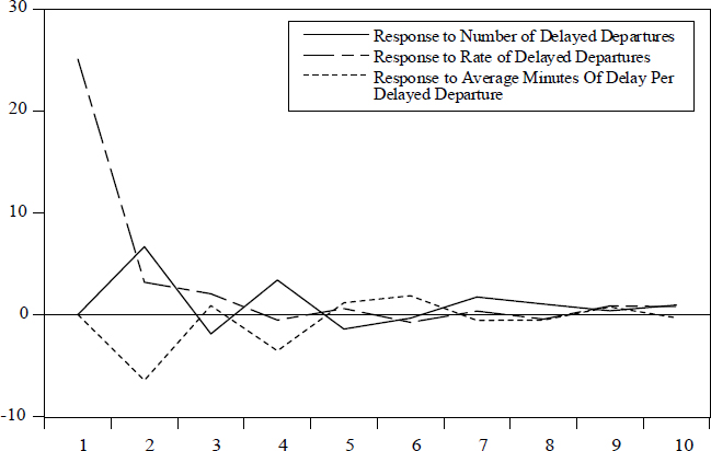
Figure 8 indicates that the fluctuation of series I has the greatest impact on itself. A standard deviation disturbance has a great impact on its delay of 1 hour. As time goes on, the impact weakens. After the delay of 5 hours, it rises again, it continues to decline after the delay of 6 hours, until the impact basically disappears after the delay of 8 hours. The series III is affected by the fluctuation of series I and reaches the peak in the 4th hour. It has a negative impact on the series II, which increases in reverse direction and reaches the peak value in 4 hours, then fluctuates slightly in 5 hours and finally disappears in 9 hours. Based on the impulse response function chart, it can be concluded that series I and series III have a positive impact on series I and can be maintained for about 7 hours.

Figure 8

Impulse response analysis affected by delayed departures

Figure 9 demonstrates that the fluctuation of series II has the greatest impact on itself, and a standard deviation disturbance has a great impact on its lag of 1 hour. However, in the second hour, the impact quickly weakens and has a negative impact, which remains stable within 4 to 8 hours and disappears after 10 hours. After 5 hours, it rose again, and then continued to decline after 6 hours lag. After 8 hours, the effect basically disappeared. The impact of series I increased rapidly from 1 hour to the maximum value and remained stable after that. The impact on series III of departure flight is small, which increases to the maximum slowly in 4 hours, then decreases slowly and disappears in 9 hours.

Figure 9

Impulse response analysis affected by the rate of delayed departure

Figure 10 explains that the fluctuation of the series III has the greatest impact on itself, and a standard deviation disturbance has a great impact on its 1-hour delay, but in the second hour, the impact is rapidly weakened and eliminated in 4 hours. The fluctuation had an impact on series I and series III in 2 hours, but the impact decreased slowly with time and disappeared after 9 hours.

Figure 10

Impulse response analysis affected by average delay time of departure flight

4.3.3 The variance decomposition of VAR model

Variance Decomposition analyzes the variance composition of prediction errors in the VAR model, which is the relationship between a certain part of the variance and the variable. Variance decomposition is used to express the dynamic characteristics of the model.

Based on the VAR (8) model, setting the forecast period is 10 hours, the variance decomposition of the forecast error is shown in Figure 11, Figure 12 and Figure 13.

Figure 11

Variance decomposition of prediction error of delayed departures

Figure 12

Variance decomposition of prediction error of the rate of delayed departures

Figure 13

Variance decomposition of prediction error of average delay time of departure flight

In the first six hours, the error comes from the proportion of itself gradually decreases with time, and finally reaches 80%. The error comes from the proportion of series II and series III gradually increases with time. The proportion of final series II is 15%, and the proportion of series III is 5%.

In Figure 11, the blue line is the variance of series I caused by its own change, the red line is caused by the change of series II, and the green line is caused by the change of series III.

The variance decomposition of prediction error of series II is shown in Figure 12.

In Figure 12, the proportion of error in the first four hours from itself gradually decreases with time, and finally stabilizes to 30%; the proportion of error in the first six hours from series III gradually increases with time, and finally stabilizes to 7%. In the first two hours, the proportion of series II gradually increased with time, and finally stabilized to 63%.

The variance decomposition of the prediction error of the series III is shown in Figure 13.

In Figure 13, the proportion of the error in the first two hours from itself gradually decreases with time, and finally stabilizes to 90%. The proportion of the error in the first one hour from series II gradually increases with time, and finally stabilizes to 6%. In the first two hours, the proportion of series I gradually increased with time, and finally stabilized to 4%.

In summary, when using the model to predict, we need to pay attention to the influence of other endogenous variables on the prediction variables. For the prediction of the above three flight delay time series, we should pay attention to the interaction between different sequences.

4.3.4 Comparison of prediction results

Use VAR model to explore the predictability of flight delay time series. Compared with AR and ARCH models, the Root Mean Square Error (RMSE) of the results are shown in the Table 6.

Table 6

RMSE of prediction results of time series in different models

Time series	VAR	AR	ARCH
I	5.4273	8.5743	6.3572
II	9.8978	13.2587	10.4514
III	23.7859	28.4175	24.4542
IV	5.521	9.8478	6.7218
V	10.7833	14.2149	11.1274
VI	26.1687	30.5685	27.7418

As can be seen from the Table 6, the RMSE of prediction results of the VAR model is the smallest, indicating that the error is the lowest, which means that the VAR model is superior to other models.

5 Conclusion

This paper constructs the flight delay time series and analyzes the characteristics of the time series. The main work of this article consists of three parts. The first part introduces the analysis of research results related to flight delays, and analyzes the problems in the research. The second part proposes methods for analyzing the characteristics of flight delay time series, and points out the key technologies of these methods. Finally, the experiments and results are analyzed, and the conclusions about the characteristics of flight delay time series are pointed out.

This paper focuses on the key technologies as follows.

Using the K-means algorithm to cluster the sequences and divide it into five categories for analyzing.
Exploring the fractal characteristics of time series by using the fractal theory. The Hurst index values are all between the interval (0.5, 1), indicating that the time series have good fractal characteristics. And the memory length V of the sequence is mostly 15, indicating that the delay condition in current will affect the delay condition within the next 15 hours.
Designing the VAR model. Firstly, the IRF is used to reflect the dynamic influence of each delay rate time series. Then, Variance Decomposition is used to explore the specific sources of variance generation.

The conclusions above show that the future development trend can be predicted by the fluctuation of current time series, and the prediction of flight delay can be realized.

Acknowledgement

This work was supported in part by the joint funds of National Natural Science Foundation of China and Civil Aviation Administration of China (U1933108), the Scientific Research Project of Tianjin Municipal Education Commission (2019KJ117), and the Fundamental Research Funds for the Central Universities of China (3122020076 and 3122019051)

References

[1] Wang Yuan, Hu Minghua and Xu Donghui, Study on the characteristics of airport surface operation delay, Journal of Wuhan University of Technology, vol. 43(Jan 2017), no. 1, 448-453.Search in Google Scholar

[2] Zhang Zhaoning and Wang Jinghua, State space model of large area flight delay propagation in airport, Science and technology and engineering, vol. 18(Feb 2018), no. 31, 241-245.Search in Google Scholar

[3] Haiyan C, Jiandong W and Tao X U, A Flight Delay State-Space Model Based on Delay Propagation, Information and Control, vol. 21(Apr 2012), no. 2, 245-277.Search in Google Scholar

[4] Liu Yujie, Prediction of flight delay and impact based on Bayesian network, Ph. D dissertation. Tianjin University, Tianjin, 2009Search in Google Scholar

[5] Dershowitz N and Manna Z, Inference Rules for Program Annotation, Transactions on Software Engineering, vol. 7(2006), no. 2, 207-222.10.1109/TSE.1981.234518Search in Google Scholar

[6] Long D and Hasan S, Improved Predictions of Flight Delays Using LMINET2 System-Wide Simulation Model, Aiaa Aviation Technology, Integration, & Operations Conference, 2013, 145-151.Search in Google Scholar

[7] Rebollo J J and Balakrishnan H, Characterization and prediction of air traffic delays, Transportation Research Part C: Emerging Technologies, vol. 44(Feb 2014), no. 3, 231-241.10.1016/j.trc.2014.04.007Search in Google Scholar

[8] Kabir S R, Allayear S M and Alam M M, et al., A computational technique for intelligent computers to learn and identify the human’s relative directions, ICISS, India, 2017, 1037-1040.10.1109/ISS1.2017.8389336Search in Google Scholar

[9] Liu Xiaofei, Research on flight delay prediction model and method based on data mining, Nanjing University of Aeronautics and Astronautics, Ph.D. dissertation, Nanjing 2010.Search in Google Scholar

[10] Zhang Jing, Study on airport capacity and delay assessment of weather impact Nanjing University of Aeronautics and Astronautics, Ph.D. dissertation, Nanjing, 2012.Search in Google Scholar

[11] Luo Jianqian, Chen Zhijie, Tang Jinhui, et al., Flight delay prediction using support vector machine regression, Transportation system engineering and information, vol. 15(Oct. 2015), no. 1, 143-149.Search in Google Scholar

[12] Yang Xinqian, Wang Qian, Liu Jun and Zhang Baocheng, Prediction of flight delay combination in the era of big data, Chinese science and technology paper, vol. 11(Nov. 2016), no. 19, 2205-2208 + 2242.Search in Google Scholar

[13] Hua Shanshan, Analysis and prediction of departure abnormal flight characteristics of Capital International Airport, China Civil Aviation University, Ph.D. dissertation Tianjin, 2017.Search in Google Scholar

[14] Hu Chao, An Empirical Study on domestic flight delays, Chongqing University, Ph.D. dissertation, Chongqing, 2017.Search in Google Scholar

[15] Wu Renbiao, Li Jiayi and Qu Jingyi, Flight delay prediction model based on dual channel convolutional neural network, Computer application, vol. 335(Dec. 2008), no. 07, 276-282 + 288.Search in Google Scholar

Received: 2020-04-30

Accepted: 2020-08-12

Published Online: 2020-12-01

This work is licensed under the Creative Commons Attribution 4.0 International License.

Articles in the same Issue

https://doi.org/10.1515/jisys-2020-0045

Keywords for this article

Delay characteristic analysis; K-means algorithm; Fractal characteristics; VAR

Creative Commons

BY 4.0