Integrating AI and genomics: predictive CNN models for schizophrenia phenotypes
-
Guilherme Henriques

 ,
Daniel Martins
and
Joel P. Arrais
,
Daniel Martins
and
Joel P. Arrais

Abstract
This study explores the use of deep learning to analyze genetic data and predict phenotypic traits associated with schizophrenia, a complex psychiatric disorder with a strong hereditary component yet incomplete genetic characterization. We applied Convolutional Neural Networks models to a large-scale case-control exome sequencing dataset from the Swedish population to identify genetic patterns linked to schizophrenia. To enhance model performance and reduce overfitting, we employed advanced optimization techniques, including dropout layers, learning rate scheduling, batch normalization, and early stopping. Following systematic refinements in data preprocessing, model architecture, and hyperparameter tuning, the final model achieved an accuracy of 80 %. These results demonstrate the potential of deep learning approaches to uncover intricate genotype-phenotype relationships and support their future integration into precision medicine and genetic diagnostics for psychiatric disorders such as schizophrenia.
1 Introduction
Schizophrenia (SCZ) is a complex and multifaceted psychiatric disorder that impacts millions globally, leading to substantial disability and imposing a heavy strain on affected individuals, their families, and healthcare system [1], 2]. It is characterized by disruptions in cognition, emotion, and perception, and its multifactorial nature – stemming from genetic, environmental, and physiological factors – poses significant challenges for effective diagnosis and treatment [3]. To address these challenges, a robust approach combining genomics, epidemiology, bioinformatics, and clinical research is necessary [4]. Research into the genetic basis of SCZ has shown a vital hereditary component, with family and twin studies estimating a heritability rate of approximately 80 % [5], 6]. Although considerable research has been conducted, the precise genetic contributors to SCZ remain elusive. Numerous genes, particularly those regulating neurotransmitter pathways – such as dopamine, glutamate, and GABA – have been implicated as potential susceptibility factors. Nonetheless, their exact contributions to the onset and progression of SCZ require further elucidation [7], [8], [9], [10]. This persistent ambiguity underscores the intricate nature of the disorder and necessitates the adoption of more sophisticated methodologies to dissect its genetic foundations. SCZ is clinically diagnosed primarily through the assessment of characteristic symptoms, including hallucinations, delusions, cognitive deficits, and social disengagement. However, these manifestations exhibit substantial variability across individuals and frequently overlap with symptoms of other psychiatric conditions, complicating the diagnostic process [11]. Misdiagnosis is not uncommon, and this not only delays appropriate treatment but also complicates efforts to elucidate the genetic mechanisms underlying SCZ [12], 13]. In response, several large-scale case-control studies, particularly those conducted in Scandinavian countries, have sought to better understand the biological aspects of SCZ by focusing on its genetic risk factors [14], 15].
In the past decade, machine learning (ML) has gained traction as a powerful approach for analyzing and interpreting complex biological data, including genetic data [16], [17], [18]. ML models have the ability to detect intricate patterns in large genomic datasets that might be overlooked by traditional statistical methods [19], 20]. This capability makes ML particularly well-suited for studying complex diseases like SCZ, where multiple interacting genetic and environmental factors are at play [21], 22].
The application of ML in psychiatry has shown great potential in helping the early diagnosis of SCZ. By analyzing genetic profiles, environmental exposures, and clinical history, ML algorithms can identify individuals at high risk for developing SCZ [23], 24]. These predictive models hold the potential to revolutionize clinical practice by facilitating earlier and more precise diagnoses. This advancement paves the way for personalized treatment approaches tailored to an individual’s specific risk profile [25], 26].
The main goal of this research is to develop a computational model that utilizes ML algorithms to identify genetic patterns linked to SCZ just based on genetic data [25], 26]. By optimizing data preprocessing techniques and leveraging existing biological knowledge, we seek to improve the accuracy and interpretability of our models, thus contributing to a deeper understanding of the genetic mechanisms underlying SCZ. The Python code used in this study is available at https://github.com/larngroup/CNNSCZ.
2 Methods
2.1 Convolutional Neural Network (CNN) model architecture
This study utilizes a Convolutional Neural Network Architecture, a deep learning model tailored for processing data with grid-like topology, commonly employed for image and pattern recognition tasks [27]. CNNs are highly efficient for feature extraction due to their hierarchical structure, low number of trainable parameters compared to fully connected networks, and adaptability in learning abstract data representations [28]. This architecture has been expanded to applications beyond images, including genomic sequence data, which exhibits a regular grid structure, making CNNs well-suited for this task [29].
The proposed model is structured with multiple layers, each playing a crucial role in identifying complex patterns within genomic data. The model architecture comprises two convolutional layers, each seamlessly integrated with a max-pooling layer to reduce dimensionality and minimize overfitting effectively. This configuration enables the model to capture intricate and broader genomic patterns while preserving a compact and efficient design. As shown in Figure 1, the CNN starts with a 2-dimensional (2D) convolutional layer, ideal for handling the structured input data despite the dataset’s one-dimensional nature since 2D convolutions allow for better spatial feature extraction. A 2D convolutional layer was chosen to capture the spatial patterns in the genomic data, even though our dataset is one-dimensional, meaning that the DNA sequences are represented as linear strings. The 2D approach is ideal for this case because, in the 1D one, the model would only be able to scan along the length of the sequence, which would limit the model’s ability to detect the interactions between more distant regions; however, by using a 2D convolution, we can reshape the 1D data by organizing the genomic sequences into smaller segments, allowing the model to learn patterns across both the sequence and different features (segments) simultaneously, ending up learning both local dependencies and higher order spatial relationships [30].
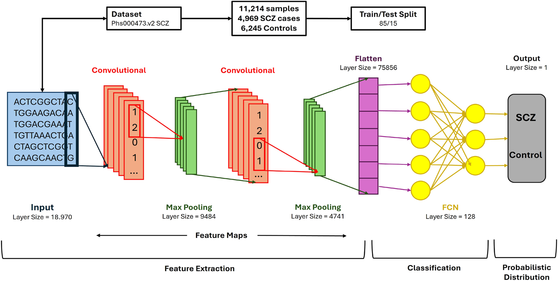
Convolutional Neural Network Structure: the designed architecture efficiently extracts patterns in genomic data to predict outcomes based on genome variants of each individual.
The addition of more than one convolutional layer allows the network to learn a hierarchical feature representation. Early layers focus on understanding simple patterns, such as edges or basic genomic motifs, while deeper layers capture more complex features, such as interactions between genetic variants [31]. To further mitigate underfitting, additional convolutional layers were incorporated, thus increasing the feature learnability by deepening the network structure [32].
Max-pooling layers, placed after each convolutional layer, are crucial in reducing the spatial dimensions of the feature maps, which aids in controlling overfitting by summarizing regions of the input [33]. These pooling layers enhance the network’s ability to generalize by down-sampling the feature maps, making the network less sensitive to minor variations in the input data, a typical issue in biological datasets [34].
Finally, after the convolution and pooling layers, a fully connected (FC) layer is included to aggregate the extracted features and pass them to the output layer for classification [35]. The FC layer transforms the multidimensional feature maps into a one-dimensional vector, which is subsequently used for classification tasks. The output layer uses a softmax activation function to predict the class probabilities, such as the presence or absence of a genetic condition, based on the input genome variants [36].
Once the architecture is implemented, the model undergoes training using a labeled dataset, and its performance is evaluated using metrics such as accuracy and loss. These metrics are indicative of the model’s predictive capability and efficiency in classifying genomic data [37]. Further refinements, such as hyperparameter tuning and regularization, are applied to optimize the network’s performance during training [38].
2.2 Dataset and preprocessing
In this study, we utilized data from the Sweden Schizophrenia Population-Based Case-Control Exome Sequencing dataset, which is stored in the dbGaP repository [39] under the accession ID code phs000473.v2.p2. The dataset includes information for 12,380 individuals, consisting of 6,245 controls and 6,135 cases. Of the cases, 4,969 were diagnosed with SCZ, while 1,166 were diagnosed with bipolar disorder. However, for the purposes of this study, only the SCZ cases were analyzed to maintain a binary classification framework. Participants in both the case and control groups were required to be at least 18 years old, with both parents born in Scandinavia [40], [41], [42]. Participants for the study were selected through data from the Swedish Hospital Discharge Register. To qualify, individuals need to have been hospitalized on at least two separate occasions, with each admission confirming a diagnosis of schizophrenia (SCZ). Any individuals diagnosed with other medical or psychiatric disorders that might compromise the precision or reliability of the SCZ diagnosis were not included in the research sample. Control cases were randomly selected from the general population and excluded if they had any recorded history of hospitalization for SCZ. To the best of our knowledge, this dataset represents one of the most considerable whole-exome and whole-genome sequencing resources available for studying schizophrenia, accessed through request.
The initial dataset comprised 1,811,204 variants, all of which had a call Phred-score (QUAL) above 30 [43]. For this study, BCFtools [44], along with its fill-tags plugin, was utilized to remove the bipolar samples from the dataset and to recalculate key metrics for each variant site, including mean read depth (DP), Allele count (AC), Number (AN), and frequency (AF). Further filtering was carried out using VCFTools (Version 0.1.15) [45], applying criteria such as allele count (AC = 0), depth (DP < 8), and a genotype call rate lower than 90 %. Multi-allelic variants were segregated with BCF tools. For newly identified variants, genotypes that were neither the reference nor the alternative allele were marked as missing. A second round of filtering was applied to the split variants, adhering to the same conditions: allele count (AC = 0), depth (DP < 8), and genotype call rate under 90 %. The Variant Quality Score Recalibration process from the Genome Analysis Toolkit Best Practices Workflow (Version 3.8) [46] was followed to guarantee variant call accuracy.
In order to explore potential relationships between genotypic variation and phenotypic expression, chi-squared tests were performed utilizing a 3 × 3 contingency framework, accommodating the three possible genotypic categories across both case and control groups. Variants located on sex chromosomes, as well as insertion-deletion polymorphisms (InDels), were deliberately excluded to maintain consistency and reliability in the statistical assessment. The resulting p-values were reported without correction for multiple testing. This decision was made to preserve a broader spectrum of genetic variants for subsequent evaluation, reducing the likelihood of overlooking variants that may exert meaningful biological influence. By adopting this more inclusive strategy, the analysis allowed for a more exhaustive examination of potential genotype-phenotype associations. After filtering, the dataset contained 18,970 variants, which were then annotated using the most up-to-date version of Annovar [47], aligned to the hg19 genome RefSeq [48], as of October 19, 2021. The annotated variants spanned 9,160 unique genes.
3 Results and model optimization
The model development involved multiple trial and error stages, spanning approximately 43 h (2,550 min) of testing. After each test, the results were analyzed to identify potential issues or factors affecting the model’s performance. The initial code was more straightforward and less structured, but the model’s precision improved significantly with subsequent parameter tuning and the addition of layers and techniques. Visual representations, such as graphs, were used to illustrate the model’s output and performance effectively. The results are explained below based on the different stages of model refinement.
3.1 Initial model testing
In the first version, we allocated 99 % of the data for training and only 1 % for testing. While this model achieved an accuracy of 100 % with an impressively low loss value of 4.9557 × 10⁻⁵ %, these results were achieved within 6–9 training epochs. This raised concerns about overfitting, as such rapid convergence often indicates that the model may not generalize well to new data. To counter this, we explored parameter adjustments and model architecture modifications, aiming to improve its ability to generalize effectively.
3.2 Optimized data split and architectural refinements
Through a series of adjustments, we achieved more reliable results. We modified the data split to allocate 85 % for training and 15 % for testing, reduced the layer sizes, and increased the number of epochs from 15 to 20. Additionally, we expanded the number of neurons in the fully connected network (FCN) from 100 to 500. To improve clarity, we also simplified the way predictions were displayed, making performance analysis more intuitive. These refinements resulted in a more steady accuracy progression over epochs, with the loss value stabilizing at approximately 2 %. However, despite these improvements, around 50 % of the predictions remained incorrect, highlighting the need for further optimization.
3.3 Parameter optimization and additional refinements
To further enhance the model, we increased the number of epochs to 100 and introduced a new parameter: the percentage of data used for predictions. Additionally, we added an extra neuron layer to the FCN, incorporated dropout in both the max-pooling layers and the FCN, and implemented a function for graphical result visualization. These modifications led to more stable training performance, with accuracy and loss following expected trends. The testing accuracy improved to 68 %, while the prediction error rate decreased to 10 %. However, despite these enhancements, graphical analysis of the testing set still suggested the presence of overfitting, albeit at a reduced level.
3.4 Overfitting reduction and model optimization
To further minimize overfitting, we simplified the FCN by removing its second neuron layer and introduced an optimization technique. We tested both the “adam” and “SGD” optimizers and ultimately chose “adam” since the performance difference between the two was negligible. The modifications led to noticeable improvements in the testing set graphs, with smoother accuracy and loss curves showing fewer fluctuations. Accuracy saw a slight increase of approximately 1 %, while the prediction error dropped from 10 % to 8 %. Additionally, incorporating early stopping allowed the model to assess performance at each epoch and discard those that did not contribute to accuracy gains. This adjustment further stabilized the loss and accuracy curves, leading to more consistent and reliable performance.
3.5 K-Fold cross-validation and model adjustments
Following extensive testing, we introduced modifications to the model by incorporating a third dimension of size three, where each layer corresponded to a specific genotype (0, 1, and 2) [49]. Instead of using pre-trained weights, genotype-specific values were assigned, while the remaining layers were initialized with zeros. These adjustments produced accuracy and loss values comparable to previous tests, with slight improvements in learning curves. However, overfitting persisted, prompting the integration of K-fold cross-validation [50].
Even with the implementation of K-fold cross-validation, graphical analyses continued to indicate the presence of overfitting. Since the modifications did not make substantial improvements, we began exploring alternative approaches to enhance model generalization.
3.6 Final model
To further enhance performance, we experimented with various regularization methods, including Drop Blocks [51] and Spatial Dropouts. However, these approaches had minimal impact on the model’s performance. We also tested an attention mechanism [52] to improve both accuracy and interpretability, but the results did not show significant improvements. Ultimately, we opted to integrate Batch Normalization across most layers while maintaining dropout rates at 0.5.
One of the key breakthroughs came from implementing a Learning Rate Schedule, which dynamically adjusted the learning rate between epochs. This strategy helped address the early plateau observed with early stopping, leading to a notable improvement. As a result, model accuracy increased to 76 %, and the learning curves demonstrated better convergence, indicating enhanced stability during training.
In the final phase of model development, we introduced a Learning Rate Reduction function that dynamically decreased the learning rate when progress stagnated. To simplify the architecture, we used a single neuron layer with 1,000 neurons and reduced the number of filters. These refinements led to the highest recorded accuracy of 80 % (see Figure 2).
The learning curves for both the training and testing sets showed significant improvements, reflecting a more balanced ratio of correct to incorrect predictions and a noticeable reduction in overfitting. To evaluate the impact of different model configurations on performance, we tested several combinations of model dimension, filter sizes, and batch sizes. The results, presented in Table 1, highlight the most effective setups for both 2D and 3D CNNs. Additionally, we investigated the influence of varying neuron counts in different layers across both architectures. As shown in Table 2, increasing the number of neurons yielded only marginal improvements in accuracy, with no significant gains beyond a certain threshold.
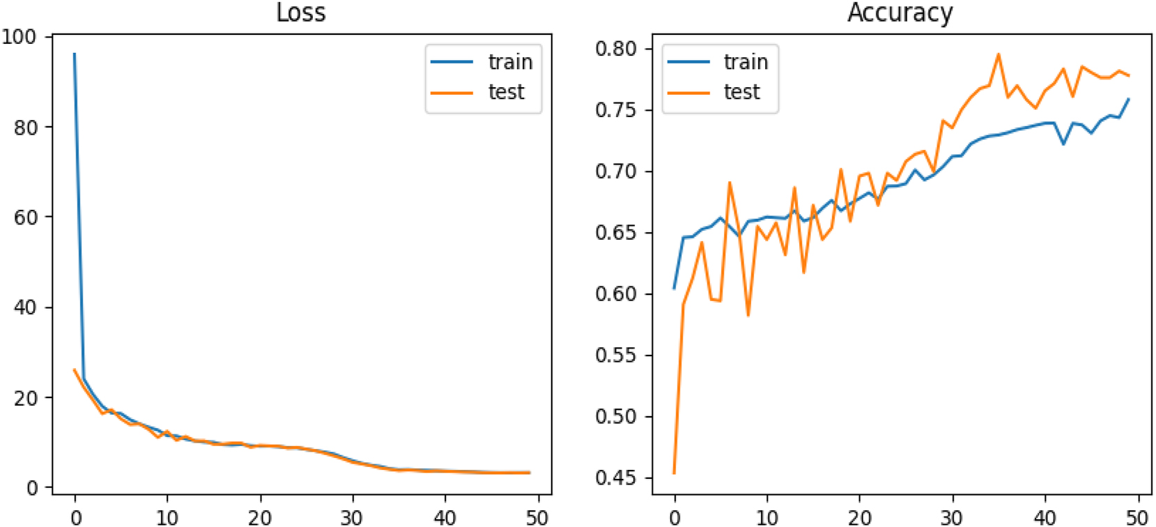
Performance evaluation of the final 2D model over 50 epochs, incorporating a single neuron layer with 1,000 neurons, a learning rate schedule, and a learning rate reduction function. The figure illustrates model accuracy, prediction error percentage, and learning curves for both training and testing sets.
Analysis of different model configurations, including variations in model dimension (MD), filter sizes, and batch sizes, and their impact on performance.
| ID | MD | Filters | Batch size | Train Acc. | Test Acc. | Observations |
|---|---|---|---|---|---|---|
| 1 | 2D | 64 | 64 | 99.56 | 72.06 | Baseline reference |
| 2 | 2D | 32 | 32 | 96.93 | 70.39 | Best parameter combination |
| 3 | 2D | 64 | 32 | 99.9 | 72.29 | Highest accuracy for both sets |
| 4 | 2D | 32 | 64 | 99.51 | 71.28 | Second-best results |
| 5 | 2D | 64 | 32 | 86.28 | 69.08 | Reference for ID – 3 |
| 6 | 2D | 64 | 32 | 99.39 | 64.1 | K-fold validation applied to ID – 3 |
| 1 | 3D | 64 | 64 | 91.56 | 70.89 | Highest test accuracy in 3D |
| 2 | 3D | 64 | 64 | 98.42 | 69.42 | Best train-test accuracy balance |
| 3 | 3D | 32 | 32 | 90.45 | 70.22 | Lowest overall accuracy |
| 4 | 3D | 64 | 32 | 90.8 | 70.49 | 3D model reference: ID – 2 |
| 5 | 3D | 32 | 64 | 92.78 | 70.44 | K-fold applied to 3D model: ID – 2 |
Effect of varying neuron counts in different layers for 2D and 3D CNN structures. MD: Model Dimension, N1: Neurons in layer 1, N2: Neurons in layer 2, Tr. Acc.: Train Accuracy, Ts. Acc.: Test Accuracy, Obs.: Observations.
| ID | MD | N1 | N2 | Tr. Acc. | Ts. Acc. | Obs. |
|---|---|---|---|---|---|---|
| 1 | 2D | 500 | 100 | 98.76 | 70.34 | Minimal impact on accuracy |
| 2 | 2D | 1,000 | 500 | 99.12 | 71.56 | Slight improvement observed |
| 3 | 2D | 1,000 | 1,000 | 99.34 | 71.89 | No significant accuracy gain |
| 4 | 3D | 500 | 100 | 92.45 | 69.78 | Lowest recorded accuracy |
| 5 | 3D | 1,000 | 500 | 93.67 | 70.12 | Minor improvement noted |
| 6 | 3D | 1,000 | 1,000 | 94.23 | 70.01 | No significant impact observed |
4 Conclusions
This study successfully developed and refined a Convolutional Neural Network (CNN) model for predicting phenotypic traits from genotypic data, with a specific focus on schizophrenia (SCZ). Through iterative improvements in data partitioning, model architecture, and regularization techniques, we achieved a notable accuracy of 80 %. This represents a significant step forward in applying deep learning to complex genetic analysis and disease prediction.
A key contribution of this research is the application of CNNs to psychiatric genetics, leveraging their hierarchical structure to detect patterns in genomic data that traditional methods might overlook. The incorporation of dropout layers, learning rate scheduling, and early stopping mechanisms helped optimize model performance by reducing overfitting and enhancing generalization.
Despite these advancements, challenges remain. Overfitting persists to some extent, and the model still exhibits a 20 % prediction error rate. These limitations suggest that while the model provides a strong foundation for genotype-to-phenotype prediction in SCZ, further refinement is essential to improve robustness and potential clinical applications.
In summary, this study adds to the expanding body of research focused on the application of deep learning methodologies within the domain of precision medicine. Ongoing improvements in predictive accuracy and model interpretability are expected to play a critical role in facilitating earlier diagnostic processes and in supporting the development of tailored therapeutic approaches for complex genetic conditions, including schizophrenia.
Funding source: FCT - Fundação para a Ciência e a Tecnologia
Award Identifier / Grant number: CEECINST/00077/2021
Award Identifier / Grant number: UIDB/00326/2025
Award Identifier / Grant number: UIDP/00326/2025
Acknowledgements
The datasets used in this manuscript were obtained from dbGaP at http://www.ncbi.nlm.nih.gov/gap through dbGaP accession number phs000473.v2.p2. Samples used for data analysis were provided by the Swedish Cohort Collection supported by the NIMH grant R01MH077139, the Sylvan C. Herman Foundation, the Stanley Medical Research Institute and The Swedish Research Council (grants 2009-4959 and 2011-4659). Support for the exome sequencing was provided by the NIMH Grand Opportunity grant RCMH089905, the Sylvan C. Herman Foundation, a grant from the Stanley Medical Research Institute and multiple gifts to the Stanley Center for Psychiatric Research at the Broad Institute of MIT and Harvard.
-
Research ethics: Not applicable.
-
Informed consent: Not applicable.
-
Author contributions: All authors have accepted responsibility for the entire content of this manuscript and approved its submission. G.H. implemented the code and wrote the first draft. D.M. helped design the model and contributed to understanding the problem. M.A. conceptualized the study, supported G.H., supervised the work, and contributed to rewriting editing the manuscript. J.P.A. supervised the research and reviewed the final version.
-
Use of Large Language Models, AI and Machine Learning Tools: Large Language Models, including ChatGPT, were used solely to improve the clarity and grammar of the manuscript text. No LLMs were involved in data analysis, results generation, or decision-making.
-
Conflict of interest: The authors state no conflict of interest.
-
Research funding: This work is financed through national funds by FCT – Fundação para a Ciência e a Tecnologia, I.P., under the framework of Projects UIDB/00326/2025 and UIDP/00326/2025. Maryam Abbasi acknowledges national funding from FCT – Fundação para a Ciência e a Tecnologia, I.P., through the institutional scientific employment program-contract (CEECINST/00077/2021).
-
Data availability: Not applicable.
References
1. Organization, WH. Schizophrenia factsheet. Geneva, Switzerland: WHO Publications; 2019.Search in Google Scholar
2. Patel, V, Farmer, P. The global burden of mental disorders. Lancet Psychiatr 2020;7:124–31.Search in Google Scholar
3. Brown, RJ, Green, T. Personalized medicine and mental health. J Psychiatr Res 2018;45:178–92.Search in Google Scholar
4. Smith, A. Comprehensive approaches to psychiatric genetics. Annu Rev Genet 2019;37:89–110.Search in Google Scholar
5. Harris, K. Twin studies in schizophrenia. J Genet Psychol 2021;55:300–12.Search in Google Scholar
6. Black, P, White, C. Genetic insights into psychiatric disorders. Nat Genet 2017;48:456–60.Search in Google Scholar
7. Green, V, Taylor, S. Dopamine and glutamate in schizophrenia. Neurobiol Rep 2019;28:501–12.Search in Google Scholar
8. Kim, L, Seo, JW, Yun, S, Kim, M. Role of GABAergic systems in schizophrenia. Front Psychiatr 2022;14:345–60. https://doi.org/10.3389/fpsyt.2023.1232015.Search in Google Scholar PubMed PubMed Central
9. Henderson, B. The dopamine hypothesis revisited. J Neurosci Res 2020;50:290–301.Search in Google Scholar
10. Gea, F. Epigenetics in psychiatric disorders. Epigenome Rev 2022;12:300–15.Search in Google Scholar
11. Rea, W. Diagnostic challenges in schizophrenia. Clin Psychiatr J 2020;50:140–55.Search in Google Scholar
12. Johnson, A. Overlapping symptoms in psychiatric disorders. Adv Psychiatr Diagn 2022;27:220–30.Search in Google Scholar
13. O’Connor, B. Schizophrenia misdiagnosis and clinical outcomes. J Clin Med 2023;18:115–25.Search in Google Scholar
14. Anderson, J. Case-control studies in schizophrenia. Scand Psychiatr Rev 2020;11:65–78.Search in Google Scholar
15. Olsen, P. Biological focus in SCZ studies. Nord Med J 2021;29:88–96.Search in Google Scholar
16. Nguyen, H. Machine learning in genomics. Bioinf Adv 2020;17:412–28.Search in Google Scholar
17. Patel, R. AI in biological data analysis. Artif Intell Med 2019;23:101–15.Search in Google Scholar
18. Gomez, F. Genetic variants and disease. Genom Res Lett 2021;34:200–15.Search in Google Scholar
19. Chen, Y. Early detection of SCZ through ML. Comput Psychiatr 2022;14:97–110.Search in Google Scholar
20. Silverman, T. AI approaches in psychiatric genetics. J Mach Learn Healthc 2022;9:45–58.Search in Google Scholar
21. Lee, A, Thompson, J. Predictive models for psychiatric genetics. J Mach Learn Health 2023;9:45–58.Search in Google Scholar
22. Rivera, S. Genetic patterns in SCZ. Med Genomics J 2020;25:330–42.Search in Google Scholar
23. Zhang, W. Modelling SCZ scenarios. J Comput Med 2021;19:189–202.Search in Google Scholar
24. Miller, J. AI in personalized healthcare. Artif Intell Med 2020;35:55–67.Search in Google Scholar
25. Garcia, L. Genetic pattern identification in SCZ. Comput Biol J 2023;19:30–50.Search in Google Scholar
26. Wang, X. Genomic data simulation for psychiatric studies. J Biomed Inf 2023;76:245–60.Search in Google Scholar
27. LeCun, Y, Bottou, L, Bengio, Y, Haffner, P. Gradient-based learning applied to document recognition. Proc IEEE 1998;86:2278–324. https://doi.org/10.1109/5.726791.Search in Google Scholar
28. Krizhevsky, A, Sutskever, I, Hinton, GE. Imagenet classification with deep convolutional neural networks. Adv Neural Inf Process Syst 2012;25:1097–105.Search in Google Scholar
29. Angermueller, C, Pärnamaa, T, Parts, L, Stegle, O. Deep learning for computational biology. Mol Syst Biol 2016;12:878. https://doi.org/10.15252/msb.20156651.Search in Google Scholar PubMed PubMed Central
30. Gu, J, Wang, Z, Kuen, J, Ma, L, Shahroudy, A, Shuai, B, et al.. Recent advances in convolutional neural networks. Pattern Recogn 2018;77:354–77. https://doi.org/10.1016/j.patcog.2017.10.013.Search in Google Scholar
31. Zeiler, MD, Fergus, R. Visualizing and understanding convolutional networks. In: European Conference on Computer Vision. Cham: Springer; 2014:818–33 pp.10.1007/978-3-319-10590-1_53Search in Google Scholar
32. Simonyan, K, Zisserman, A. Very deep convolutional networks for large-scale image recognition. arXiv preprint arXiv. 2014:14091556.Search in Google Scholar
33. Boureau, YL, Ponce, J, LeCun, Y. A theoretical analysis of feature pooling in visual recognition. In: Proceedings of the ICML. Madison, WI, USA: Omnipress; 2010.Search in Google Scholar
34. Scherer, D, Müller, A, Behnke, S. Evaluation of pooling operations in convolutional architectures for object recognition. In: International Conference on Artificial Neural Networks. Berlin, Heidelberg: Springer; 2010:92–101 pp.10.1007/978-3-642-15825-4_10Search in Google Scholar
35. Goodfellow, I, Bengio, Y, Courville, A. Deep learning. Cambridge, Massachusetts, United States: The MIT Press; 2016.Search in Google Scholar
36. Bishop, CM. Pattern recognition and machine learning. New York: Springer; 2006.Search in Google Scholar
37. Hastie, T, Tibshirani, R, Friedman, J. The elements of statistical learning: data mining, inference, and prediction. Heidelberg, Germany: Springer Science & Business Media; 2009.Search in Google Scholar
38. Bergstra, J, Bardenet, R, Bengio, Y, Kégl, B. Random search for hyper-parameter optimization. J Mach Learn Res 2012;13:281–305.Search in Google Scholar
39. Tryka, KA, Hao, L, Sturcke, A, Jin, Y, Wang, ZY, Ziyabari, L, et al.. NCBI’s database of genotypes and phenotypes: DbGaP. Nucleic Acids Res 2014;42:D975–9. https://doi.org/10.1093/nar/gkt1211.Search in Google Scholar PubMed PubMed Central
40. Ripke, S, O’dushlaine, C, Chambert, K, Moran, JL, Kähler, AK, Akterin, S, et al.. Genome-wide association analysis identifies 13 new risk loci for schizophrenia. Nat Genet 2013;45:1150–9. https://doi.org/10.1038/ng.2742.Search in Google Scholar PubMed PubMed Central
41. Purcell, SM, Moran, JL, Fromer, M, Ruderfer, D, Solovieff, N, Roussos, P, et al.. A polygenic burden of rare disruptive mutations in schizophrenia. Nature 2014;506:185–90. https://doi.org/10.1038/nature12975.Search in Google Scholar PubMed PubMed Central
42. Genovese, G, Fromer, M, Stahl, EA, Ruderfer, DM, Chambert, K, Landén, M, et al.. Increased burden of ultra-rare protein-altering variants among 4,877 individuals with schizophrenia. Nat Neurosci 2016;19:1433–41. https://doi.org/10.1038/nn.4402.Search in Google Scholar PubMed PubMed Central
43. Ewing, B, Hillier, L, Wendl, MC, Green, P. Base-calling of automated sequencer traces using Phred. I. Accuracy assessment. Genome Res 1998;8:175–85. https://doi.org/10.1101/gr.8.3.175.Search in Google Scholar PubMed
44. Danecek, P, Bonfield, JK, Liddle, J, Marshall, J, Ohan, V, Pollard, MO, et al.. Twelve years of SAMtools and BCFtools. GigaScience 2021;10. https://doi.org/10.1093/gigascience/giab008.Search in Google Scholar PubMed PubMed Central
45. Danecek, P, Auton, A, Abecasis, G, Albers, CA, Banks, E, DePristo, MA, et al.. The variant call format and VCFtools. Bioinformatics 2011;27:2156–8. https://doi.org/10.1093/bioinformatics/btr330.Search in Google Scholar PubMed PubMed Central
46. Van der Auwera, GA, Carneiro, MO, Hartl, C, Poplin, R, Del Angel, G, Levy-Moonshine, A, et al.. From FastQ data to high-confidence variant calls: the genome analysis toolkit best practices pipeline. Current Protoc Bioinform 2013;43. https://doi.org/10.1002/0471250953.bi1110s43.Search in Google Scholar PubMed PubMed Central
47. Wang, K, Li, M, Hakonarson, H. ANNOVAR: functional annotation of genetic variants from high-throughput sequencing data. Nucleic Acids Res 2010;38:e164. https://doi.org/10.1093/nar/gkq603.Search in Google Scholar PubMed PubMed Central
48. O’Leary, NA, Wright, MW, Brister, JR, Ciufo, S, Haddad, D, McVeigh, R, et al.. Reference sequence (RefSeq) database at NCBI: current status, taxonomic expansion, and functional annotation. Nucleic Acids Res 2016;44:D733–45. https://doi.org/10.1093/nar/gkv1189.Search in Google Scholar PubMed PubMed Central
49. Liu, Y, Wang, D, He, F, Wang, J, Joshi, T, Xu, D. Phenotype prediction and genome-wide association study using deep convolutional neural network of soybean. Front Genet 2019;10:1091. https://doi.org/10.3389/fgene.2019.01091.Search in Google Scholar PubMed PubMed Central
50. Anguita, D, Ghelardoni, L, Ghio, A, Oneto, L, Ridella, S. The ‘K’ in K-fold cross validation. In: Proceedings of the European Symposium on Artificial Neural Networks, Computational Intelligence and Machine Learning (ESANN). Bruges, Belgium: ESANN; 2012:441–6 pp.Search in Google Scholar
51. Ghiasi, G, Lin, TY, Le, QV. DropBlock: a regularization method for convolutional networks. In: Advances in Neural Information Processing Systems (NeurIPS). Montréal, Canada: NeurIPS; 2018:10727–37 pp.Search in Google Scholar
52. Zhang, L, Zhang, L, Song, J, Gao, L. A survey of capsule network architectures and applications. Neurocomputing 2021;450:274–93.Search in Google Scholar
© 2025 the author(s), published by De Gruyter, Berlin/Boston
This work is licensed under the Creative Commons Attribution 4.0 International License.
Articles in the same Issue
- Frontmatter
- Workshops
- Predicting precursors of plant specialized metabolites using DeepMol automated machine learning
- Fcodes update: a kinship encoding framework with F-Tree GUI & LLM inference
- Towards a more accurate and reliable evaluation of machine learning protein–protein interaction prediction model performance in the presence of unavoidable dataset biases
- Leveraging transformers for semi-supervised pathogenicity prediction with soft labels
- Survival risk prediction in hematopoietic stem cell transplantation for multiple myeloma
- Predicting DDI-induced pregnancy and neonatal ADRs using sparse PCA and stacking ensemble approach
- A ViTUNeT-based model using YOLOv8 for efficient LVNC diagnosis and automatic cleaning of dataset
- Automated mitosis detection in stained histopathological images using Faster R-CNN and stain techniques
- Colon cancer survival prediction from gland shapes within histology slides using deep learning
- Integrating AI and genomics: predictive CNN models for schizophrenia phenotypes