Capital Account Liberalization, Structural Change, and Female Employment

2.1 Female Employment Intensity Across Industries

Before turning to the empirical analysis, we begin with stylized facts on the female intensity of employment across sectors. Table 1 presents the average female employment shares by countries’ income level and six broadly defined industrial sectors. We sort sectors by their tradability. Overall, female intensity is the highest in the public sector. However, female intensity in different sectors also varies by development level. While agriculture is the most female intensive sector in low income countries, the public sector has the highest female employment share in the rest of the country groups.

The second part of Table 1 presents the average female employment shares in tradable and nontradable sectors. In the econometric specifications, our tradability variable is a continuous variable. However, by using the value added tradability score index (TSVAX) by Bykova and Stöllinger (2017), we classify sectors that have higher tradability score than 0.15 as tradable sectors, and the rest as the nontradable sectors. In Table 1, the first three sectors belong to tradable sectors, and the rest are nontradable sectors. Low income countries also have different pattern than the rest when we look at the average female intensity in tradable and nontradable sectors. While female intensity is higher in tradable sectors in low income countries, overall nontradable sectors are more female intensive for the rest of the countries.

Figure 1 shows the conditional means of female employment shares in different income groups in tradable sectors. Two salient features emerge from the figure. First, female intensity in tradable sectors is the highest in low income countries and lowest in high income countries. Second, female intensity is remarkably constant throughout the sample.

Figure 1:

Average female employment shares in tradables by income group. World Bank country classifications by income level: L, low income; LM, lower-middle income; UM, upper-middle income; H, high income.

3.1 Alternative Specifications

Given the large effects reported above, we subject our results to a series of robustness exercises, as reported in Table 2. These include specifications with country-specific time trends (column 2), sector-specific time trends (columns 3 and 6), and additional control variables (columns 4–6). The latter consist of the logarithm of population, in order to account for country level trends in labor supply, financial openness and the current account balance as a percent of GDP, to control for the level of capital account openness and capital flows around a liberalization episode. We also allow for sector heterogeneity in the control variables by interacting the controls with sector dummies (columns 5–6). The large and persistent negative effect on female employment is present and significant in most specifications, though the exact magnitude varies, ranging from a lower bound of 12 % to an upper bound of 30 % after 8 years.

3.2 Within and Between Sector Decomposition

We now dig deeper and decompose the overall effect on female employment into the contribution of within sector changes in the female intensity of employment and the contribution of employment reallocation between sectors. Let θ ijt = ℓ ijt f / ℓ ijt refer to the female intensity in sector j, where ℓ ijt f and ℓ _ijt denote female and overall employment in sector j, respectively. Defining the log cumulative difference Δ _h x _t  = ln x _t+h  − ln x _t−1, the overall cumulative response of female employment can be decomposed as.

Equation (2) simply states that the cumulative change in female employment Δ h ℓ ijt f is equal to the sum of the cumulative change in female intensity Δ _h θ _ijt and sector employment Δ _h ℓ _ijt . Accordingly, we estimate the local projection in equation (1) using each element of the decomposition as the dependent variable in order to uncover the contribution of each term.

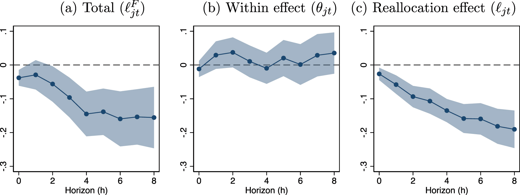
The benchmark decomposition results are reported in Figure 3. As a reference, panel (a) reports the overall effect already discussed above. The contributions of the within sector and reallocation terms are shown in panels (b) and (c), respectively. Consistent with equation (2), at each horizon the impulse responses in panels (b) and (c) must sum to the overall impulse response in panel (a).

Figure 3:

Decomposition of female employment effect. Note: This figure reports the impulse response of female employment to sectoral exposure to a liberalization episode (LIB _i  × TI _j ). Panel (a) reports the overall cumulative response for total female employment in sector j. Panels (b) and (c) decompose the total response into the contribution of changes in the female employment intensity within a sector and the contribution of sectoral employment reallocation. The shaded areas depict the 95 % confidence interval, which were calculated with heteroskedasticity and autocorrelation consistent (HAC) standard errors.

Perhaps surprisingly, the large effect on overall female employment appears to be primarily driven by sector reallocation effects (panel c). In contrast, the within sector effects on the female intensity of employment (panel b) are modest and statistically insignificant at most time horizons. These results are consistent with a strong form of gender segregation in tradable industries and suggest that the aggregate response of female employment to capital account liberalization is mostly due to resulting structural change, as opposed to changes in the gender composition of employment within sectors.

3.3 Sensitivity to Tradability Measure

Because the definition of tradability plays a central role in the results described above, we carry out a series of sensitivity tests using alternative tradability indexes and sectoral classifications. Specifically, we estimate the same specification as in Figure 3 but replace our exposure variable. These are reported in Table 3. Row (a) reports the overall effect on female employment 4 years after a liberalization episode, while rows (b) and (c) report the within and reallocation components, respectively. Columns (1)–(2) reports results with continuous tradability indexes. The first is our benchmark specification (column 1), which considers a time invariant tradability index. Column (2) reports the results using a time-varying measure of tradability. Next, columns (3)–(4) consider binary sector classifications. In column (3) we define the tradable sector as consisting of agriculture, manufacturing, and mining, while in column (4) we define the tradable sector as consisting of only manufacturing.

As reported in Table 3, the decomposition results are similar regardless of which tradability measure is employed. The reallocation effect in row (c) dwarfs the within sector composition effect across most specifications. The exception is when manufacturing is treated as the sole tradable sector. As can be seen in column (4), in this case the contributions of within sector changes in female intensity are sizable and statistically significant.

3.4 Income Group Heterogeneity

As an additional sensitivity exercise, we now present the decomposition results for alternative samples depending on a country’s level of development at the beginning of the sample period. This allows us to check if structural differences between the poorest and the rest of the countries in the sample entail qualitatively different results. In particular, we carry out separate decompositions for countries classified as “low-middle income” and the poorest “low income” and report the cumulative impulse response of each decomposition component 8 years after exposure to a liberalization shock.^[4]

The results are as follows. As can be seen in column (1) of Table 4, on average, the decline in female employment is primarily driven by the between sector employment reallocation effect (line c). However, breaking up the sample reveals meaningful heterogeneity between low-middle income (column 2) and the poorest low income (column 3) countries. While the reallocation effect is the driving force for low-middle income countries, changes in within sector female intensity appear to matter much more for low income countries. Indeed, in low income countries the within sector effect is nearly three times as large as the reallocation effect and statistically significant. The overall effect on female employment is also larger for low income countries, with female employment declining nearly 40 % in tradable sectors 8 years after a financial liberalization shock.

4.1 Household Problem

We first present the simple version of our model. In this version, labor supply is fixed and we ignore home production. In the extended version, we will relax the assumption of fixed labor supply and consider unpaid care/household work. We consider a classical economy with full employment:

where l j g is the employed labor in each sector j = T, N for each genders g = f, m. In a full employment economy, total demand for labor is equal to the exogenous supply of labor ( L ̄ ) .

Households are identical in our model and choose to maximize their utility subject to their budget constraint. Households have Cobb–Douglas preferences defined over both goods:

where α ∈ (0, 1). Households earn wages from working and profits from the firms. They face the following budget constraint:

where w j g is the wage earned by gender g in sector j, and Π denotes aggregate profits. Here, NX refers to net exports and is exogenous by assumption. We will use this variable below to capture the effect of capital account liberalization.^[6]

As is standard in two-sector models, the optimality condition is given by:

which states that the representative household equates the marginal rate of substitution to the relative price of nontradable goods.

4.2 Firms

Labor is the only factor of production in both sectors. Nontradable and tradable sectors have different production technologies. In the nontradable sector, the production technology is constant returns to scale and the production function can be expressed as

where θ N = ℓ N f ℓ N , denotes the female employment ratio in the nontradable sector and is assumed to be constant. This assumption can be interpreted as a form of strict occupational segregation in terms of gender. Firms’ problem in the nontradable sector is to choose labor to maximize their profits:

where the optimal solution is such that price is a weighted average of female and male wages in the nontradable sector:

The tradable sector’s production technology is decreasing returns to scale and in the following form:

where A > 0 is a productivity shifter, and θ T = ℓ T f ℓ T is the female employment share in the tradable sector and is also assumed to be constant. Thus, the tradable sector is also assumed to feature strict gender-based occupational segregation. Firms in the tradable sector also choose labor to maximize their profits:

The solution gives us the optimal demand for labor, which equalizes the marginal product of labor to the weighted average of wages in the tradable sector,

Perfect labor mobility between sectors implies that a given gender will earn the same wage across sectors. However, wages between genders need not equalize in equilibrium due to the presence of strict occupational segregation. We assume that women have a wage penalty and are paid as a proportion (η < 1) of the male wage. Using this parameter, we can redefine female wages in terms of male wages:

4.3 Aggregate Constraints

To find the economy’s aggregate constraints, we rewrite the budget constraint (6) as follows:

where we made use of the definition of aggregate profit income Π and the full employment condition. If we divide both sides by p _T , we get

Market clearing in the nontradable sector requires the supply to equal demand y _N  = c _N . This implies that the aggregate constraint for the tradable sector is simply given by:

4.4 Equilibrium

An equilibrium in this economy consists of (i) consumption choices c ^T and c ^N , (ii) labor allocation decisions ℓ j g for g = f, m and j = T, N, and (iii) prices p N , w f , w m that

1. solve the household’s problem;

2. maximize firm profits;

3. satisfy the occupational constraints (i.e.  ℓ T f / ℓ T = θ T );

4. ensure all markets clear.

4.5 Solution

The general equilibrium in this model can be characterized as follows. We combine the aggregate constraints in both sectors, the first order condition from the household’s problem, and the full employment condition to obtain:

Noting that ℓ T f = θ T ℓ T and normalizing the total labor supply L ̄ = 1 , we can express this condition as:

we will refer to equation (19) as the “market clearing” condition or “MC-schedule.”

Next, we can rearrange the first order conditions of firms in equations (10) and (13) as follows using the wage equations ( w N f = w T f = w f = η w m and w N m = w T m = w m ):

Combining these equations, we obtain the following condition:

where we have defined:

We will refer to (22) as the “labor return” or “LR-schedule” because it is this condition that ensures that effective labor returns are equalized between sectors.

It is worth taking a moment to examine the variable z in the LR schedule, which summarizes the impact of the gender-based occupational segregation across sectors. As can be seen in equation (23), the constant z acts as a wedge on the relative marginal products of both sectors and depends on the gender composition of employment in each sector (θ _N and θ _T ) and on the relative female wage η.

Now that we have reduced the economy to the MC and LR schedules, we have obtained a system of two equations with two unknowns: the real exchange rate q and female employment ℓ T f . It can be readily verified that the MC schedule is upward sloping in ℓ T f , q -space while the LR schedule is downward sloping. This is represented graphically in Figure 4, along with a typical equilibrium at point A . Thus, in our framework the RER and the composition of employment are determined simultaneously in general equilibrium.

Figure 4:

General equilibrium – female labor.

4.6 Effect of Capital Inflows

Although we abstract from intertemporal saving and borrowing decisions, we can nevertheless model the macroeconomic effects of a surge of capital inflows as a decrease in the exogenous level of net exports NX. This is arguably a good approximation of the effects of financial liberalization in developing countries.^[7] According to equation (19), there is a negative relationship between net exports and the real exchange rate in the MC schedule. As shown in Figure 4, a drop in net exports (↓NX) leads to an upward shift in the MC curve. The new equilibrium occurs at point B . Thus, the RER appreciates and female employment in the tradable sector shrinks. If the female employment share in the tradable sector is larger than the male employment share, reallocation of women’s employment would be higher than men’s.

A few remarks are in order. First, the equilibrium RER appreciation obtained above could be avoided or attenuated by external policy interventions, such as foreign reserve accumulation. In this sense, the comparative statics depicted in Figure 4 should be regarded as holding constant any other policy interventions that are expected to affect the RER. Second, financial liberalization has historically been associated with increased volatility and a higher likelihood of experiencing a currency crisis.^[8] In other words, financial liberalization could very well result in RER depreciation if followed by a crisis. The model presented here thus abstracts from these considerations.

4.7 Consequences of a Change in Relative Female Wages

How does the structure of gender-based occupational segregation affect the macroeconomic outcomes in our model? We start by examining the effect of exogenous changes in the female wage penalty. Taking the partial derivative of q with respect to η in the LR schedule, we obtain:

The sign will depend on the sign of the numerator, specifically θ _N  − θ _T . Since this is a small economy model, we can consider two different cases for low and low-middle income countries. In the first case, we focus on low income countries. In low income countries, female intensity is higher in the tradable sector (θ _T  > θ _N ) as shown in Table 1, so we can conclude that ∂ q ∂ η < 0 . Graphically, this corresponds to a downward shift in the LR schedule, as shown in Figure 5. As can be seen in the figure, as the female wage penalty decreases (when η increases), the real exchange rate depreciates and female employment in tradables falls, corresponding to a movement from the original equilibrium at point A to the new equilibrium at point B .

Figure 5:

Decreasing female wage penalty (↑η).

In the second case, we focus on low-middle income countries. In the low-middle income countries, the nontradable sector is more female-intensive (θ _N  > θ _T ) as shown in Table 1, so ∂ q ∂ η > 0 . In this case, as a result of a decrease in the female wage penalty (an increase in η), the real exchange rate appreciates and female employment in tradables increases. However, we should also mention that the difference between the female employment share in tradables and nontradables, only 1 % according to Table 1, is very small. Therefore, the size of the effect would be smaller than the case in the low income countries.

When female intensity is higher in the tradable sector, as is the case for the low income countries, the female wage penalty will overwhelmingly affect this sector. A decreasing wage penalty therefore disproportionately increases the effective wage costs of tradable firms. As a result, the tradable sector shrinks and the real exchange rate depreciates. As the income level of the country increases female intensity in tradable sectors declines relative to the one in nontradable sectors. Therefore, the effect of a change in the female wage penalty might be in the opposite direction. In low-middle income countries, even though female intensity is higher in nontradables, the difference is very small. Hence, the effects might be relatively small.

5.1 Model Solution

The supply-side of the model remains unchanged from the previous section. Profit maximization by N-sector firms (10) implies q = (1 − (η − 1)θ _N )w ^m , where we have used w ^f  = ηw ^m . Plugging in the value of q into (29) and combining with (30) and (25), we can solve for the labor supply of each household member:

where we have used the market clearing condition c _N  = y _N and have defined the constant:

It immediately follows that the aggregate labor supply is:

The household’s labor supply functions depend on the level of consumption of nontradables y _N , the female wage gap η, and the minimum home production requirements, κ ^f and κ ^m . Intuitively, higher consumption of nontradables increases the marginal utility of consuming home goods, which increases the amount of time devoted to home production and consequently leads to a decrease in household labor supply. As can be seen in equation (31), this channel will be weaker for female labor supply due to existence of a female wage gap η < 1.

5.2 Relative Female Employment

An important feature of this model extension is the possibility of an endogenous aggregate female to male employment ratio driven by macroeconomic conditions and, in particular, structural change between tradables and nontradables. This feature is desirable because it makes it possible to relate our framework to the existing empirical literature, which tends to focus on aggregate female employment gaps.^[10] Two factors make this feature possible: (i) the inclusion of the minimum home good input requirements κ ^g , which render the resulting labor supply functions non-homothetic and (ii) the existence of a female wage penalty η < 1, which attenuates the response of female labor supply to changes in y _N .

Using (31), we can define the ratio of female to male labor supply G = ℓ ^f /ℓ ^m as:

which may be increasing or decreasing in y _N depending on the values of η, κ ^m , and κ ^f .^[11] It can be verified that dG/dy _N < 0 when the following condition is satisfied:

This condition states that an expansion in the nontradable sector will lower female employment relative to male employment as long as women’s burden in home good production is disproportionately high (that is, when κ ^f is sufficiently large). It is worth noting that if the gender wage gap is absent (η = 1), this condition reduces to simply κ ^f  > κ ^m , in which case an expansion of nontradables always reduces the ratio of aggregate female to male labor supply.

5.3 General Equilibrium

To solve for the equilibrium supply of nontradables, recall that y _N  = ℓ _N , which implies that the full employment condition can be expressed as L = ℓ _T  + y _N . Combining the full employment condition with the aggregate labor supply (32) and solving for y _N , we get:

The equilibrium supply of nontradables can therefore be expressed as a decreasing function of the labor employed in the tradable sector: y _N  = y _N (ℓ _T ), with y N ′ ( ℓ T ) < 0 .

Armed with the above equilibrium relationships, we can characterize the general equilibrium link between the RER q, female employment in the T-sector ℓ T f , and the relative female employment ratio G = ℓ ^f /ℓ ^m in terms of three equations:

where we have again used the relation ℓ T f = θ T ℓ T . Equation (36) is the MC schedule modified to account for an endogenous aggregate labor supply, while (37) is the familiar LR schedule equating the marginal products of labor across sectors. As above, the MC schedule is upward sloping in ℓ T f , q -space while the LR schedule is downward sloping. The third equation (38) denotes the equilibrium relative female employment expressed as a function of ℓ T f . We therefore have a system of three equations defined over three unknowns q , ℓ T f , G .

The general equilibrium is depicted graphically in Figure 6. As in the previous section, the MC and LR schedule (in the upper panel) together uniquely pin down the equilibrium RER and employment structure q , ℓ T f , while the relative female employment ratio G is determined recursively by ℓ T f (in the lower panel). Here, we have assumed that the burden of home production falls disproportionately on women and that condition (34) holds.^[12]

Figure 6:

RER and employment structure in general equilibrium.

5.4 Financial Liberalization

We conclude by reexamining the effects of financial liberalization, modeled as an exogenous rise in capital inflows and the associated deterioration in net exports NX. As above, the capital inflows increase consumption of the tradable goods, leading to a RER appreciation. As shown in the top panel of Figure 6, this entails to an upward shift in the MC schedule and shrinking female employment in tradables, corresponding to a transition from equilibria A to B . In other words, the implications of financial liberalization for structural change and female employment in the tradables is qualitatively unaffected by endogenizing the labor supply choice.

What does qualitatively change, however, is the response of the aggregate female to male employment ratio G = ℓ ^f /ℓ ^m . As can be seen in the bottom panel of Figure 6, when the tradable sector shrinks in response to a surge of capital inflows, aggregate female employment disproportionately decreases relative to male employment. This is indicated by a movement from points C to D . As already noted, this result assumes that the burden of home production falls disproportionately on women, which is arguably the empirically relevant case.

Put differently, the model predicts that large RER appreciations should have larger effects on female employment than on male employment. Similarly, in this framework a competitive RER undervaluation should be expected to disproportionately stimulate female employment, which is consistent with the empirical results reported by Erten and Metzger (2019).

References

Agenor, Pierre-Richard. 2007. “The Analytics of Segmented Labor Markets.” In Adjustment Policies, Poverty, and Unemployment: The IMMPA Framework, Chapter 1, edited by Pierre-Richard Agenor, Alejandro Izquierdo, and Henning Tarp Jensen, 8–66. Wiley-Blackwell.Search in Google Scholar
Borrowman, Mary, and Stephan Klasen. 2020. “Drivers of Gendered Sectoral and Occupational Segregation in Developing Countries.” Feminist Economics 26 (2): 62–94. https://doi.org/10.1080/13545701.2019.1649708.Search in Google Scholar
Braunstein, Elissa, and Mark Brenner. 2007. “Foreign Direct Investment and Gendered Wages in Urban China.” Feminist Economics 13 (3–4). https://doi.org/10.1080/13545700701439432.Search in Google Scholar
Braunstein, Elissa, and James Heintz. 2008. “Gender Bias and Central Bank Policy: Employment and Inflation Reduction.” International Review of Applied Economics 22 (2). https://doi.org/10.1080/02692170801889643.Search in Google Scholar
Bykova, Alexandra, and Roman Stöllinger. 2017. “Tradability Index: A Comprehensive Measure for the Tradability of Output.” wiiw Statistical Report (6).Search in Google Scholar
Caraway, Teri L. 2006. “Gendered Paths of Industrialization: A Cross-Regional Comparative Analysis.” Studies in Comparative International Development 41 (1): 26–52. https://doi.org/10.1007/bf02686306.Search in Google Scholar
Chinn, Menzie D., and Hiro Ito. 2006. “What Matters for Financial Development? Capital Controls, Institutions, and Interactions.” Journal of Development Economics 81 (1). https://doi.org/10.1016/j.jdeveco.2005.05.010.Search in Google Scholar
Domínguez-Villalobos, Lilia, and Flor Brown-Grossman. 2010. “Trade Liberalization and Gender Wage Inequality in Mexico.” Feminist Economics 16 (4). https://doi.org/10.1080/13545701.2010.530582.Search in Google Scholar
Erten, Bilge, and Martina Metzger. 2019. “The Real Exchange Rate, Structural Change, and Female Labor Force Participation.” World Development 117. https://doi.org/10.1016/j.worlddev.2019.01.015.Search in Google Scholar
Erten, Bilge, Anton Korinek, and José Antonio Ocampo. 2021. “Capital Controls: Theory and Evidence.” Journal of Economic Literature 59 (1): 45–89. https://doi.org/10.1257/jel.20191457.Search in Google Scholar
Evelyn, F. Wamboye, and Stephanie, Seguino. 2015. “Gender Effects of Trade Openness in Sub-Saharan Africa.” Feminist Economics 21 (3).10.1080/13545701.2014.927583Search in Google Scholar
Furceri, Davide, Prakash Loungani, and Jonathan D. Ostry. 2019. “The Aggregate and Distributional Effects of Financial Globalization: Evidence from Macro and Sectoral Data.” Journal of Money, Credit and Banking 51 (1). https://doi.org/10.1111/jmcb.12668.Search in Google Scholar
Ghosh, Atish R., Mahvash Qureshi, Jun Il Kim, and Juan Zalduendo. 2014. “Surges.” Journal of International Economics 92: 266–85. https://doi.org/10.1016/j.jinteco.2013.12.007.Search in Google Scholar
Ghosh, Atish R., Jonathan D. Ostry, and Mahvash Qureshi. 2016. “When Do Capital Inflow Surges End in Tears?” American Economic Review: Papers & Proceedings 106: 581–5. https://doi.org/10.1257/aer.p20161015.Search in Google Scholar
Ghosh, Atish R., Jonathan D. Ostry, and Mahvash Qureshi. 2017. Taming the Tide of Capital Flows: A Policy Guide. Massachusetts Institute of Technology.10.7551/mitpress/9780262037167.001.0001Search in Google Scholar
Harris, John, and Michael Todaro. 1970. “Migration, Unemployment and Development: A Two-Sector Analysis.” American Economic Review 60.Search in Google Scholar
Jorda, Oscar. 2005. “Estimation and Inference of Impulse Responses by Local Projections.” The American Economic Review 95 (1). https://doi.org/10.1257/0002828053828518.Search in Google Scholar
Kucera, David, and Sheba Tejani. 2014. “Feminization, Defeminization, and Structural Change in Manufacturing.” World Development 64: 569–82. https://doi.org/10.1016/j.worlddev.2014.06.033.Search in Google Scholar
Salter, W.E.G. 1959. “Internal and External Balance: The Role of Price and Expenditure Effects.” Economic Record 35. https://doi.org/10.1111/j.1475-4932.1959.tb00462.x.Search in Google Scholar
Saraçoğlu, Dürdane, Emel Memiş, Ebru Voyvoda, and Burça Kızılırmak. 2018. “Changes in Global Trade Patterns and Women’s Employment in Manufacturing, 1995–2011.” Feminist Economics 24 (3): 1–28. https://doi.org/10.1080/13545701.2018.1435899.Search in Google Scholar
Seguino, Stephanie. 2016. “Global Trends in Gender Equality.” Journal of African Development 18 (1): 1–30. https://doi.org/10.5325/jafrideve.18.1.0009.Search in Google Scholar
Seguino, Stephanie. 2020. “Engendering Macroeconomic Theory and Policy.” Feminist Economics 26 (2). https://doi.org/10.1080/13545701.2019.1609691.Search in Google Scholar
Seguino, Stephanie, and James Heintz. 2012. “Monetary Tightening and the Dynamics of US Race and Gender Stratification.” American Journal of Economics and Sociology 71 (3). https://doi.org/10.1111/j.1536-7150.2012.00826.x.Search in Google Scholar
Stiglitz, Joseph E. 2004. “Capital-Market Liberalization, Globalization, and the IMF.” Oxford Review of Economic Policy 20. https://doi.org/10.1093/oxrep/grh004.Search in Google Scholar
Swan, Trevor W. 1963. Longer Run Problems of the Balance of Payments. The Australian Economy.Search in Google Scholar
Tejani, Sheba, and William Milberg. 2016. “Global Defeminization? Industrial Upgrading and Manufacturing Employment in Developing Countries.” Feminist Economics 22 (2): 24–54. https://doi.org/10.1080/13545701.2015.1120880.Search in Google Scholar
© 2023 Walter de Gruyter GmbH, Berlin/Boston
Articles in the same Issue
- Frontmatter
- Editorial
- The Gendered Effects of Globalization: Recent Evidence from Developing Countries
- Research Foundation
- Protectionism and Gender Inequality in Developing Countries