Generalized Structural Mean Models for Evaluating Depression as a Post-treatment Effect Modifier of a Jobs Training Intervention

Alisa Stephens; Luke Keele; Marshall Joffe

doi:10.1515/jci-2015-0032

Article Open Access

Generalized Structural Mean Models for Evaluating Depression as a Post-treatment Effect Modifier of a Jobs Training Intervention

Alisa Stephens , Luke Keele and Marshall Joffe

Published/Copyright: July 28, 2016

Published by

Become an author with De Gruyter Brill

Submit Manuscript Author Information

From the journal Journal of Causal Inference Volume 4 Issue 2

Abstract

In randomized controlled trials, the evaluation of an overall treatment effect is often followed by effect modification or subgroup analyses, where the possibility of a different magnitude or direction of effect for varying values of a covariate is explored. While studies of effect modification are typically restricted to pretreatment covariates, longitudinal experimental designs permit the examination of treatment effect modification by intermediate outcomes, where intermediates are measured after treatment but before the final outcome. We present a novel application of generalized structural mean models (GSMMs) for simultaneously assessing effect modification by post-treatment covariates and accounting for noncompliance to assigned treatment status. The proposed approach may also be used to identify post-treatment effect modifiers in the absence of noncompliance. The methods are evaluated using a simulation study that demonstrates that our approach retains consistent estimation of effect modification by intermediate variables that are affected by treatment and also predict outcomes. We illustrate the method using a randomized trial designed to promote re-employment through teaching skills to enhance self-esteem and inoculate job seekers against setbacks in the job search process. Our analysis provides some evidence that the intervention was much less successful among subjects that displayed higher levels of depression at intermediate post-treatment waves of the study. We also compare the assumptions of our approach and principal stratification as alternatives to account for differences in effects by intermediate variables.

Keywords: post-treatment interaction; structural mean model; causal odds-ratio

1 The JOBS II study and effect modification

Evaluation is an important aspect of policy interventions such as job-training programs. Here, we evaluate the JOBS II Intervention Project developed at the University of Michigan and designed to enhance the reemployment prospects of unemployed workers [1]. The intervention aimed to teach unemployed workers skills related to searching for employment such as the preparation of job applications and resumes and how to successfully interview. An additional focus of the intervention, however, was on the mental health aspects of the job search process. This component of the training included activities to enhance self-esteem, increase a sense of self-control, and cope with set-backs. These skills were taught to help job-seekers maintain motivation and persist in the job-search process.

Of the sampled workers, the researchers randomly assigned 1,249 to the job search seminar (treatment) and 552 to the control condition, which consisted of a short pamphlet on job search strategies. Workers assigned to the treatment condition attended a 20-hour job search seminar over one week. Follow-up interviews were conducted 6 weeks, 6 months, and 2 years after the intervention. We focus on whether the intervention increased re-employment. Unlike the original analysis, we also examine how covariates measured post-treatment might be used to better evaluate the effectiveness of JOBS II. We conduct two different analyses based on post-treatment covariates.

Many previous analyses have focused on intention-to-treat (ITT) effects of participation in JOBS II [1, 2, 3, 4] (though see Jo and Vinokur [5]; Little and Yau [6]; Mattei et al. [7] exceptions). While ITT effects are important, there are other relevant causal quantities when there is noncompliance. In JOBS II only 61 % of those assigned to the intervention actually attended the training seminars, while those assigned to control could not access the treatment. It is therefore relevant to focus on whether the intervention was efficacious among those who actually attended the job search seminar, which requires conditioning on post-treatment information [8, 9].

In addition to accounting for noncompliance, we also evaluate post-treatment effect modification, an understudied use of post-treatment covariates in the analysis of randomized trials. In a randomized study of treatments, effects may be heterogenous, observed as an interaction between a treatment and an effect modifying covariate such that the average treatment effect varies across values of the covariate. For example, we can consider treatment effects that vary by covariate-defined subpopulations such as sex or race. While analyses with effect modification by a pretreatment covariate are relatively common, it is also possible for effect modification to occur as a function of a post-treatment covariate. In many randomized studies, data on post-treatment or intermediate covariates, defined as variables measured post-intervention but prior to the study endpoint, are often collected. For example in JOBS II, after treatment, intermediate measures were collected at time intervals such as six weeks and six months after treatment, whereas the final outcome measures were collected two years later. In such designs, we may suspect that the treatment effect may vary across levels of a covariate measured after the treatment but before the final outcome.

There are several reasons to consider the possibility of effect modification by a post-treatment variable. First, post-treatment effect modification can be used for intermediate decision making if the trial is ongoing. Analysts could use the model to identify subgroups for whom the treatment is particularly ineffective and a new intervention might be implemented. Second, results from an analysis of this form could also be used as a method for hypothesis-generation and the design of future interventions. Third, the model might be combined with other identification strategies to show a consistent pattern of associations in support of a causal hypothesis. Keele [10] provides one example where post-treatment effect modification is used as an alternative identification strategy to instrumental variables. In that example, similar conclusions from alternative identification strategies are used to bolster a single causal hypothesis.

Post-treatment effect modification is an important but yet unstudied aspect in JOBS II. In designing the study, effect modification by pretreatment levels of depression was of particular concern. As a result 520 unemployed workers were excluded from the overall sample of eligible subjects prior to randomization since they displayed a clinically significant level of depression [1]. This exclusion allowed the researchers to apply the intervention to the subpopulation in which it would be most effective. While job loss is known to induce depression, the original study did not consider that re-employment failures – failed interviews, a lack of call backs – may also increase levels of depressive symptoms. If re-employment failures elevated levels of depression after the intervention, the effectiveness of the treatment for this subpopulation may be reduced. We use a model of post-treatment effect modification to estimate whether post-treatment levels of depression reduced the effectiveness of the treatment.

In our analysis, we adopt the framework of potential outcomes to define causal effects based on comparisons of potential outcomes on a common set of units [11, 12]. Our primary estimand is the causal odds ratio among the treated within subgroups defined by post-treatment levels of depression. We show how our estimand may be characterized as an example of single potential outcome stratification under the principal stratification (PS) framework considering depression levels among those assigned to treatment [13]. A key contribution of our analysis is exploring and outlining identifiability conditions for this estimand. We use generalized structural mean models (GSMMs) for binary outcomes and a modified G-estimation procedure to estimate the post-treatment effect modification of the causal odds ratio among compliers [14]. While additive SMMs have been applied to post-treatment effect modification [15], we adapt them to allow for estimation in the odds-ratio scale.

Our paper has the following structure. Section 2 provides basic descriptive statistics and some preliminary analyses. Section 3 outlines our notation, describes our causal estimand, states identifiability conditions. In Section 4, we detail the estimation procedure. Section 5 evaluates the properties of the two-parameter logistic GSMM for post-treatment effect modification through a simulation study. Section 6 presents estimates of post-treatment effect modification of causal effects in JOBS II. Section 7 includes discussion and concluding remarks.

2 Descriptive summaries and preliminary analyses

For all subjects in the JOBS II study, researchers collected covariates prior to treatment assignment. Baseline covariates include education, income, sex, age, occupation, race, risk for failure, level of economic hardship, and a measure of depressive symptoms. The primary outcome of interest is a binary indicator for whether subjects were employed 20 or more hours per week at the two year follow-up period. We use all units from the original sample with nonmissing values at baseline and at intermediate data collection time points. The intent-to-treat (ITT) analysis reveals that the odds of success in the treatment arm as compared to the control arm is 1.49 with a 95 % confidence interval (1.10,2.01). This implies that for those assigned to treatment the odds of re-employment were 49 % higher. In ignoring noncompliance, the ITT estimate speaks to program effectiveness but not efficacy. We address the question of efficacy below.

Next, we examine whether levels of depression appeared to be elevated at post-treatment follow-up periods. Depressive symptoms were measured with a scale of 11 items from the Hopkins Symptom Checklist with scores ranging from 0 to 6.0. A score of 3.00 or greater on the depression index was considered to be a clinically significant indication of depression. As we noted above, subjects with scores of 3 or more were excluded from the JOBS II study prior to randomization. We re-scaled the depression scale to range from 0 to 100, which aids interpretation. On this scale, subjects with a score of 50 or higher were removed from the study. Figure 1 contains box plots of depression scores at baseline and the two follow-up periods. The measure of depression in the plot excludes all subjects who were removed due to a high level of depressive symptoms at baseline. While the median level of depression decreases at the follow-up periods, for some subjects, levels of depression are elevated well above the 50 point threshold which indicates a clinically significant level of depression in the post-treatment periods. Here, we examine whether the intervention was less effective among subjects with higher levels of post-treatment depression.

Figure 1:

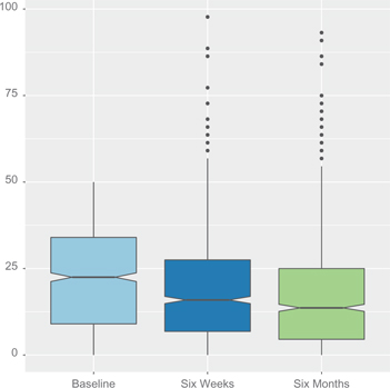
Levels of depression at baseline, the six week, and six month follow up. Scores above 50 are considered to be a clinically significant indication of depression.

3 Estimand and identification conditions in the analysis of JOBS II

Next, we describe the causal estimand of interest in the analysis of the JOBS II trial using potential outcomes structural mean models (SMMs). SMMs were developed for the analysis of randomized trials with noncompliance [9], but provide a general structure for estimating the effect of post-randomization exposures [16, 17]. We also outline the assumptions needed for identification of our estimand, since under both noncompliance and post-treatment effect modification, we condition on post-treatment quantities. Rosenbaum [18] demonstrates that conditioning on post-treatment covariates may result in biased estimates of the causal parameter. We examine the identifiability conditions for post-treatment effect modification in detail since identification assumptions under noncompliance are well-known. We conclude this section with a detailed discussion of our estimand within the PS framework [19].

3.1 Causal estimand and initial assumptions

In JOBS II, subjects (i=1,…,n) are randomly assigned to either treatment (Ri=1) or control (Ri=0). Covariates Xi=(X1,…,Xk) are measured at baseline prior to randomization, including age, race, and baseline depression. We define post-treatment effect modifiers, Si, as the set of intermediate covariates observed after treatment but prior to the outcome, also possibly multivariate. In our application, we focus on a single potential post-treatment effect modifier: level of depressive symptoms which we denote by Si. Further, to reflect the choice by subjects to comply with their treatment assignment, we denote actual exposure to the treatment by Ai. In JOBS II, those assigned to control did not have access to the training sessions in the intervention condition. Therefore when Ri=0 then Ai=0. Conversely, if Ri=1, then Ai=1 if subject i complies with treatment assignment and attends the job training seminars, and if Ai=0, the subject does not comply with treatment assignment and does not attend. The observed response, denoted by Yi and which follows self-selected exposure Ai, is an indicator of employment of 20 hours or more per week. The temporal order of observed variables is Xi,Ri,Ai,Si,Yi.

One common way to define causal effects is in terms of counterfactual or potential outcomes [12, 20, 21]. Under the potential outcomes framework, Yir,a, is the potential outcome when Ri=r and Ai=a. To estimate the causal effect of the JOBS II intervention on employment, we would like to compare how each subject would respond under treatment to his or her response under the control condition. The potential outcome under no treatment is Yir,0, and it indicates a treatment-free response that would have been observed if, perhaps counter to fact, subject i had not received treatment. We further define Ai,r and Si,r,Ai,r as potential outcomes of treatment exposure and intermediate depression under treatment assignment Ri=r.

Next, we stipulate a set of assumptions for identifiability of the effect of Ai. First, we assume that the SUTVA holds [22] which has the two following components: 1) there are no hidden forms of treatment, which implies that for unit i under Ri=r and Ai=a, we assume that Yir,a=Yi and 2) a subject’s potential outcome is not affected by other subjects’ exposures. The first component of SUTVA is often referred to as the consistency assumption in the epidemiological literature. Schwartz et al. [23] contains a discussion of the relationship between these forms of assumptions.

We assume the exclusion restriction holds which states that Yi1,0 is equal to Yi0,0, and we denote Yi0=Yi1,0=Yi0,0 [8]. The exclusion restriction implies that being invited to the job training seminar has no direct effect on the odds of re-employment two years later. It seems plausible that being invited to a training seminar itself does little to change the probability of re-employment other than through actual participation in the seminar. We assume that the treatment assignment is ignorable, defined as independence between the treatment assignment and potential outcomes under no treatment. In JOBS II, this assumption is justified by the randomized design. Formally, this restriction can be expressed as

(1)Yi0⊥Ri|Xi

Further, we assume the “no-contamination” restriction, defined as the absence of off-protocol use of the intervention among controls, such that P(Ai=0|Ri=0)=1 [24]. This assumption is justified by the design since control subjects could not access the intervention. The no contamination restriction implies the no current treatment interaction assumption for SMMs, which states that the causal effect of the intervention is identical among subjects who actually took it, regardless of assigned treatment [25], since it reduces the number of causal effects to one among those assigned to the intervention. The causal effect among those assigned to control can never be estimated, so the underlying data-generating mechanism remains agnostic about the existence of the interaction under unrestricted designs [9, 26]. We also assume that Ri has a nonzero causal effect on Ai. These assumptions will identify the effect of Ai on Yi and are equivalent to the usual instrumental variables assumptions [8]. We consider further assumptions to identify effect modification later.

To ease exposition, we denote two changes to the notation. First, we drop the index i, since throughout we assume all quantities are indexed by individual participants in the JOBS II trial. Second we denote Ar=1 as A1. That is, A1 represents the potential compliance status under fixed treatment assignment R=1. We also simplify S1,A1, the potential level of depression for a potential compliance status with fixed treatment assignment R=1, to SA1 and define YA1 similarly. In our application, we focus on treatment effect modification by SA1. Specifically, we consider the following form of effect modification by SA1 where if for some s not equal to s′

(2)E[YA1−Y0|SA1=s,R=1]≠E[Y1−Y0|SA1=s′,R=1].

In JOBS II, the primary outcome of interest is binary, so we focus on effect modification by SA1 the logistic SMM [27], which models the log-causal-odds of employment vs. unemployment among subjects randomized to treatment as a function of exposure and covariates. Under the logistic SMM, our estimand is the causal odds ratio

(3)exp(ψ)=P(Y=1|SA1,A1,R=1,X)P(Y=0|SA1,A1,R=1,X)/P(Y0=1|SA1,A1,R=1,X)P(Y0=0|SA1,A1,R=1,X).

which we allow to vary across SA1. Under a set of appropriate identification conditions, we may obtain estimates of the estimand using the following model

(4)logit{P(Y1=1|SA1,A1,R=1,X)}−logit{P(Y0=1|SA1,A1,R=1,X)}=η′s(A1,SA1)ψ0=f1(A1;ψ01)+f2(A1,SA1;ψ02),

where ψ represents the unknown causal parameter, with the truth denoted by ψ0, and ηs′(⋅) is a function of potential outcomes SA1 and A1 with dimension equal to that of ψ. We use the subscript “s” to indicate that this is a structural model, since it refers to counterfactual quantities instead of observed associations in the data. In Equation (4) the structural model is comprised of arbitrary known functions f1(⋅) and f2(⋅) up to an unknown p-dimensional parameter ψ0=(ψ01,ψ02), where p=dim(ψ01)+dim(ψ02). When ψ0= or A1=0 we assume f1(ψ01)=f2(S1;ψ02)=0 to indicate no effect of treatment, and for SA1 or ψ02=0, we assume f2(Si;ψ02)=0. We condition on Xi but by assumption we rule out structural models of the form ηs′(A1,Xi)=(A1,A1Xi)′. This is discussed in further detail in Section 3.2.

As an example, consider the case when f1(ψ01)=ψ01A1 and f2(ψ02)=ψ02A1SA1. For ψ02=0, the causal odds ratio is quantified by exp(ψ01) for all subjects, implying no effect heterogeneity. When ψ02≠0, exp(ψ01) is the causal odds ratio among the subset of subjects with SA1=0, and when ψ02≠0, the causal odds ratio for subjects with SA1=s is captured by exp(ψ01+ψ02s), which allows the effect of A1 to vary with the counterfactual SA1.

Joffe et al. [13] show that models like (4) were discussed as models with a single potential outcome stratification, in contrast with a principal stratification approach, which considers a stratification on joint potential outcomes under r=0,1. We show in Section 3.2 that model (4) is equivalent to the model

(5)logit{E[Yi|Si,Ai,Ri=1,Xi]}−logit{E[Yi0|Si,Ai,Ri=1,Xi]}=η′s(Ai,Si)ψ0=f1(Ai;ψ01)+f2(Ai,Si;ψ02),

which stratifies on the observed auxiliary variable Si [13], and falls under the class of Retrospective Structural Mean Models (RSMMs). RSMMs are characterized by exposure effects defined conditional on variables observed subsequent to treatment, in contrast with standard structural mean models [9], which define causal effects as a function of covariates observed prior to treatment. Vansteelandt [16] also considered retrospective models for assessing mediation when outcomes are binary and modeled using a logit link.

Alternatively, we could use a linear SMM, which models mean differences linearly in exposure and covariates under an identity link. For positive outcomes, we might apply the log link to estimate the causal risk ratio. When mean outcomes are close to 1, either marginally or conditionally within subgroups, modeling binary outcomes using the identity or log link may result in predicted mean outcomes that are out of range, which can cause nonconvergence or falsely reported convergence in estimation routines. The logistic SMM allows for general binary outcomes that may be common or rare.

We might compare the causal odds ratio in Equation (3) to a more familiar one

(6)P(Y=1|A1,Ri=1,X)P(Yi=0|A1,R=1,X)/P(Y0=1|A1,R=1,X)P(Y0=0|A1,R=1,X),

which only allows effect modification by X For this estimand, the structural model would be rewritten as ηs′(A1,X)ψ. Structural models of this type admit the possibility that causal odds ratio is not constant over different strata of X. The distinction between Equations (3) and (6) are made clearer in the following section where we consider questions of identifiability.

Finally, we could also consider an alternative form of effect modification

(7)E[YA1−Y0|SA1−SA0=s,R=1]≠E[Y1−Y0|SA1−SA0=s′,R=1]

This second form of effect modification allows for the effect of the intervention to vary by SA1−SA0 instead of SA1. Under this second form of effect modification, we would seek to answer whether the intervention is more or less effective among those whose intermediate levels of depression are affected by exposure to the intervention. Under the form of effect modification in 2, we are attempting to understand whether the intervention was less effective with increasing depression levels under treatment.

Under a simplified setting without noncompliance, effect modification of the type in (2) may be captured by the model

E[Y1−Y0|S1,S0,X,R=1]=γ1R+γ2RS1,

whereas effect modification of the type in (7) may be modeled by

E[Y1−Y0|S1,S0,X,R=1]=γ1R+γ2R(S1−S0).

These models are nested in the following more general model

(8)E[Y1−Y0|S1,S0,X,R=1]=γ1R+γ2RS1+γ3RS0,

which suggests that a test for the appropriateness of other model may be conducted by evaluating the hypothesis that γ3=0. In applications where the intermediate variable S is only defined among the treated, these models are equivalent. Dunn and Bentall [15] consider effect modification of this type where the intervention is assignment to therapy and the effect modifier is attachment to the therapist. Since controls patients do not receive therapy, they cannot form an attachment to a therapist. See [28] for an additional example of this type in vaccine trials.

When the effect modification variable occurs in both treatment arms and varies both under intervention and control, as it does in the JOBS II application, choosing between these two models will depend on subject matter knowledge. We argue that effect modification of the form in (2) is more relevant when interest focuses on the level of the effect modifier rather than the difference in the effect modifier caused by the intervention. As we noted above, the eligibility criteria for JOBS II excluded otherwise eligible subjects that had high levels of depression at baseline because the intervention was less likely to be effective among them. Given this, we focus on the levels of depression achieved under treatment as the effect modifier. Moreover, model (8) can only be identified under additional parametric modeling assumptions beyond those we use for identification.

3.2 Identifiability under post-treatment effect modification and noncompliance

We next consider the identifiability of SMMs with post-treatment effect modification, since identification of treatment effects for those who complied with the JOBS II holds given the assumptions stated thus far. We address identifiability under a theorem presented by Vansteelandt and Goetghebeur [17] in the context of Strong Structural Mean Models. First, we consider the following model that parameterizes the odds ratio (6), under a single binary pre-treatment effect modifier Xi,

(9)logit{E(Y|A1,R=1,X)}−logit{E(Y0|A1,R=1,X)}=ψ01A1+ψ02A1X

This model is nonparametrically identified in the sense of Robins [29] under the assumptions in Section 3.1. The log odds ratio in Equation (9) is uniquely defined in terms of observable quantities given the ignorability assumption, the consistency component of SUTVA, the no-contamination assumption, and equivalence between E[Y|A1=0,R=1,X] and E[Y0|A1,R=1,X] under the exclusion restriction.

We contrast the model in Equation (9) with an example of Equation (4) as given by:

(10)logit{E(Y|SA1,A1,R=1,Xi)}−logit{E(Y0|SA1,A1,R=1,Xi)}=ψ01A1+ψ02A1SA1

using a single binary potential post-treatment effect modifier SA1. Nonparametric identification for the above model does not hold since there are four possible nonzero effects defined by joint levels of X, and SA1, but the exchangeability assumption allows identification of only two parameters. Generally, nonparametric identifiability does not hold for models of this form, since the number of strata jointly defined by the baseline covariate, X, and potential intermediate, SA1, is greater than the number of restrictions imposed by our stated assumptions [17].

To achieve model-based identification of effect modification by SA1, we must place a restriction on the number of A1X interactions in the structural model for the effect of treatment on outcomes. To derive the model-based identifiability conditions, we consider the marginal treatment effect Δx, marginalizing over SA1 and A1X. Examination of the marginal treatment effect reveals how identification depends on observed-data constraints.

(11)Δx=∑a{∑slogit(E[Y|SA1,A1,R=1,X])−logit(E[Y0|SA1,A1,R=1,X])×P(SA1=s|A1,R=1,X)}×P(A1=a|X,R=1)=∑a∑sπsax(ψ01a+ψ02as)=π1ax(ψ01a+ψ02a)+π0ax(ψ01a)P(A1=a|X,R=1)=0+p1x(ψ01+π11xψ02),

where p1x≡P(A1=1|X,R=1) and πsax≡P(SA1=s|A1=a,X=x,R=1). Equation (11) involves two equations in two unknown quantities, ψ01 and ψ02, and has a unique solution so long as Xi predicts p1x or π11x and thus identifiability holds under the model. In sum, model-based identification holds if we restrict the number of interactions between treatment assignment and baseline covariates on the outcome in the structural model. Without this assumption, the model in Equation (10) and the following model

logit{E(Y|SA1,A1,R=1,Xi)}−logit{E(Y0|SA1,A1,R=1,X)}=ψ01A1+ψ02A1X

may fit the data equally well [17]. The essence of the identifiability problem is that since SA1 is unobserved we are forced to increase the number of observed-data constraints to identify the model, which is accomplished by enforcing the ignorability criterion within baseline covariate-defined subgroups. In short, we must assume that the complexity of the structural model occurs at a rate slower than the increase in observed-data constraints. Specifically, the treatment effects implied by interactions in the structural model must not outnumber the constraints imposed by (1). A set of assumptions that would allow for nonparametric identification of post-treatment effect modifiers has not yet been identified.

No-interaction assumptions are often used for identification of causal effects. No-interaction assumptions have been invoked with instrumental variable analysis [25], in the estimation of direct and indirect effects [16, 30, 31], and for other causal analyses [17]. Under some modeling configurations, we can partially relax this no-interaction assumption as we demonstrate next.

Consider the case where we have two binary covariates X1 and X2, and we want to estimate ψ0 in the model

(12)logit{E[Y|SA1,A1,X1,X2,R=1]}−logit{E[Y0|SA1,A1,X1,X2,R=1]}=ψ01+ψ02A1X1+ψ03A1SA1.

This model is similar to (10) but now includes effect modification by a pretreatment covariate. We re-write the ignorability assumption as

Ri⊥Y0|X1,X2.

In this model, nonparametric identification still does not hold for ψ0=(ψ01,ψ02,ψ03) since there are more nonzero effects in subgroups defined by joint levels of of SA1, X1, X2 than identifying restrictions. Under our parametric model, however, the same argument as above can be applied to establish model-based identifiability. The 3-dimensional parameter ψ0 can be identified using the additional information provided by adding X2 and its ignorability assumption. That is, the parameters in model (12) may be identified potentially assuming no interactions involving X2, but not X1. However, the parameters in the following model

(13)logit{E[Y|SA1,A1,R=1,X1,X2]}−logit{E[Y0|SA1,A1,R=1,X1,X2]}=ψ01A1+ψ02A1X1+ψ03A1SA1+ψ04A1X2+ψ05A1X1X2+ψ06ASA1X1X2+ψ07A1SA1X1+ψ08A1SA1X2

cannot not be identified, nor can any other model with parameter dim(ψ0)≥4. As in the case of the bivariate parameter above, multiple models with ψ0 of the same dimension may fit the data equally well. Therefore, the no-interaction assumption is required for some, but not all of the possible baseline covariate-treatment interactions on outcomes and will depend on the richness of the available data. This result suggests a focus on a limited number of pre-treatment effect modifiers that are considered to be the most relevant. In the JOBS II data, for example, we would want to focus on baseline depression as the critical pretreatment effect modifier given its substantive relevance. However, for pre-treatment covariates such as age or gender, we would enforce the no-interaction assumption. Finally, measures can be taken to reduce the likelihood of a violation of the no-interaction assumption by limiting heterogeneity in selected subjects, as was done in JOBS II. In general, we believe the model is still useful so long as the estimates are given an exploratory rather than confirmatory interpretation.

Given the model-based identification for effect modification by SA1, it remains to be shown that the RHS of model (4) may be expressed in terms of observed data. Under our stated assumptions, the following set of equalities hold:

P(YA1=1|SA1,A1,X)=P(YA1=1|SA1,A1,R=1,X)=P(Y=1|S,A,R=1,X).

The ignorability assumption justifies the first equality (1), while the second holds due to consistency. Similarly due to ignorability, we note that P(Y0|SA1,A1,R=1,X)=P(Y0|SA1,A1,X). Under this equivalence, we would write the causal model in (4) as:

(14)logit{E[Y|S,A,R=1,X]}−logit{E[Y0|S,A,R=1,X]}=η′s(A,S)ψ0=f1(A;ψ01)+f2(A,S;ψ02),

where we condition on the observed values A and S as opposed to conditioning on the potential outcomes A1 and SA1.

3.3 Post-treatment effect modification within the principal stratification framework

Next, we further examine our structural model for post-treatment effect modification within the framework of principal stratification [19]. Principal stratification is a popular approach for thinking about certain classes of causal effects, particularly when analysts condition on post-treatment quantities. A principal stratification with respect to a post-treatment variable is a partition of units into latent classes defined by the joint potential values of that post-treatment variable under each of the treatments being compared [32]. The PS framework often provides useful insights into causal estimands based on post-treatment variables, and we use it to clarify the estimands of interest. Both noncompliance and post-treatment effect modification have been written in the PS framework as separate concepts. Here, we consider them jointly. We should note in advance that in our example the estimands are equivalent under the SMM and PS frameworks and the identification assumptions are identical.

To fully characterize our estimand under the principal stratification approach, we consider the cases of noncompliance and post-treatment effect modification separately. Under noncompliance, our estimand is identical to the principal stratification estimand in that there are four principal strata of always-takers, never-takers, defiers, and compliers [8, 19]. In the PS framework, defiers are ruled out via the monotonicity assumption. Here, the no-contamination restriction that we adopt is a strong form of the usual monotonicity assumption and thus serves an equivalent role [26]. That is, the no-contamination restriction rules out the presence of both defiers and always-takers which allows us to identify the other two strata in the observed data. Under the PS framework, to identify causal effects, we must also assume the exclusion restriction holds, but we have already stipulated the exclusion restriction under our stated assumptions. Under noncompliance, the PS estimand is often referred to as the local average treatment effect (LATE) or the complier average causal effect (CACE). The SMM estimand is also a local estimand under the no-contamination restriction [33].

Next, we characterize post-treatment effect modification using the PS framework. For the moment, we ignore compliance, and thus we denote potential levels of depression as Sr. If S is binary, as we have defined it, there are four principal strata defined by the joint levels of S1 and S0. Following, Hsu and Small [34] we characterize these four basic strata as: “always-high” (S1=1 and S0=1), “never-high” (S1=0 and S0=0), “treatment positively affected” (S1=1 and S0=0), and “treatment negatively affected” (S1=0 and S0=1). Our estimand considers patient classes defined by levels of S1. Thus to compare our estimand to that under PS, we consider the union principal strata defined by S1=1 and S1=0, taking the union of the “always-high” and “treatment positively affected” and separately the “never-high” and “treatment negatively affected” strata. If we have both noncompliance and post-treatment effect modification as in JOBS II, this implies that there are generally eight principal strata since within each of the four noncompliance principal strata, we have two effect modification union principal strata. However, under the no contamination restriction, we assume that effects are only identifiable for the two effect modification principal strata within the complier strata.

4 Estimation

We use the Vansteelandt and Goetghebeur [14] method for the estimation of causal effects under generalized structural mean models with binary outcomes using the logit link. This estimation strategy was developed as a solution to Robins [35], which showed that the causal odds ratio could not be estimated using the same G-estimation procedure as used for identity and log links in the presence of high dimensional covariates. To facilitate the definition of mean treatment-free outcomes used in this modified version of G-estimation, the first stage of a two stage model is an association model among subjects randomized to the job search seminar treatment. A detailed argument motivating the need for the association model is described in Vansteelandt and Goetghebeur [14] and largely stems from the noncollapsibility of the logit link.

The first stage model is defined as

(15)logit(E(Y|S,A,R=1,X;β))=ηa(S,A,X;β),

for a known function ηa and unknown finite-dimensional parameter vector β, and predicted mean treatment-free outcomes are constructed as

(16)H(ψ)=expit[ηa(S,A,X;β)]−f1(A;ψ1)+f2(A,S;ψ2)

for subjects randomized to treatment, where f1(A;ψ1) and f2(A,S;ψ2) are defined as in model (10) and S represents intermediate depression at either 6 weeks or 6 months. The subscript a distinguishes the association model from the structural, causal model. The functional form for ηa(S,A,X;β) is generally linear in the parameters but may include main effects, interactions, and higher order terms for the variables. For subjects randomized to control and hence unable to access treatment, the observed outcome Y equals the treatment free outcome Y0 following the consistency assumption. In the control arm, it is therefore unnecessary to estimate H(ψ) by removing the treatment effect from a model-predicted mean outcome; H(ψ) is simply set to H(ψ)=Y.

The second stage of estimation then defines the estimating function

(17)U(S,A,R,X,H(ψ))=d(X,R)H(ψ)−q(X),

for d(X,R), a p−dimensional weight function defined such that its elements d1(X,R),...dp(X,R) are non-collinear, and q(X), a function of baseline covariates. The causal parameter ψ is estimated as the solution to ∑i=1nU(S,A,R,X,H(ψ))=0. By the randomization assumption, under the true ψ and β, E∑i=1nU{S,A,R,X,H(ψ)}=0 for U(S,A,R,X,H(ψ)) as defined in (17). The chosen d(X,R) and q(X) affect efficiency but not bias in the resulting estimate ψˆ when the association model is correctly specified. Under a misspecified association model, the robust estimating equations referenced above are constructed through strategic selection of d(X,R) and guarantee that type I error is preserved. Term q(X) does not affect bias under correct or incorrect specification of the association model. Vansteelandt and Goetghebeur [14] recommend the choice d(X,R)=d∗(X)(−1)RR∗P(R=1|X)+(1−R)(1−P(R=1|X)), with d∗(X)=E∂H(ψ)∂ψ|X, following semiparametric optimality arguments for their GSMM under known β. Under the logit model ∂H(ψ)∂ψ=H(ψ)(1−H(ψ))[R/RS] where H(ψ) is evaluated at an initial estimate of ψ, ψˆb.

Under the null hypothesis ψ0=0, one may construct locally robust estimating equations that yield consistent inference under misspecified association models. For variance estimation the sandwich variance estimator that jointly considers estimation of components of the structural and association models is used, thus taking into account the estimation of the association model parameters [14].

5 Simulation study

A simulation study was conducted to evaluate the proposed estimator for assessing effect modification by post-treatment variables while also accounting for noncompliance. A second set of simulations which we show in the Appendix displays the results of a simulation study for using this approach to evaluate post-treatment effect modification under full compliance. These additional simulations also explore the impact of misspecification of the association model.

For each subject, independent baseline covariates X1∼Bernoulli(p=0.4) and X2∼Bernoulli(p=0.7) were generated. Binary treatment R was simulated following an unstratified randomization design, with R∼Bernoulli(p=0.5). A compliance variable A was generated following the model logit(P(A=1|X1))=logit(0.9)−3X1. For subjects with R=0, we set A=0 following the setting where subjects randomized to control are unable to access active treatment. Under this design, compliance was approximately 66 % among those randomized to treatment. The post-treatment variable S was simulated from the model logit(P(S=1|A,R,X))=γ0+γ1X1+γ2X2+γ3A, with γ=(logit(0.2),1.0,1.0,γ3), with γ3=0, 0.3, or 1.2 for Si not associated, weakly associated, or strongly associated with A. The data design contained binary covariates to ensure compatibility among various stages of conditional mean treatment-free potential outcome models. Each simulated dataset consisted of n=5,000 subjects.

Outcomes were generated under a likelihood consistent with the Retrospective Structural Mean Model (14), which conditions on observed posttreament data and was shown to be equivalent to model (4) that conditions on the potential intermediates using a modification of the strategy described in Robins and Scharfstein [36]. The conditional mean of Y0 given baseline covariates was defined as logit(E[Y0|X1,X2])=ρ0X+ρ1XX1+ρ2XX2+ρ3XX1X2, with ρX=(logit(0.35),0.8,−0.8,1.5). Conditional mean treatment-free potential outcomes were then adjusted for S, by setting E[Y0|S,R,X]=expit[logit(E[Y0|X1,X2])+ρ1SS+ρ0jS(1−S)], where ρ1S=0.4, and for given ρX, γ and values of covariates R,X1,X2, ρ0jS was the solution to ES[E[Y0|S,R,Xi]]=E[Y0|Xi] for j=1,...,8, indexing unique profiles of R,X1,X2. Under ignorable noncompliance we set E[Y0|Si,Ai,Ri,Xi]=E[Yi,0|Si,Ri,Xi] and simulated observed outcomes as Bernoulli(pY), where logit(py)=logit(E[Y0|S,A,R,X])+ψ1A+ψ2AS for ψ0=(0.5,–0.5). Under non-ignorable non-compliance E[Y0|S,A,R,X] was generated by adjusting the conditional treatment-free mean E[Y0|R,X] for compliance A and then S while maintaining compatibility across conditional means. Observed outcomes were then generated after incrementing mean treatment-free outcomes for the effect of observed compliance to treatment, also with ψ=(0.5,−0.5).

The application of the two-stage GSMM considered the association model fully saturated for S,A,X1,X2. The GSMM estimates were compared to estimates from two logistic regression models: model 1 was similar to an intent-to-treat analysis with the addition of post-intervention covariates and contained terms R and RS with full saturation for S,X1,X2; and model 2 was an as-treated approach, including A and AS, also with full saturation for S,X1,X2. All results were based on 1,000 replicated datasets.

Table 1:

Simulation study results. Mean estimates, percent bias, and Monte Carlo standard deviations of the modified G-estimation and standard logistic regression when ignorable noncompliance is present. ρX=(characterizes the association between baseline covariates X, and (γ1,γ2) characterize the association of X and S. γ3 is the coefficient of A in the data-generating model for S. ρ=0 indicates that S does not predict Y0. The first row in each parameter configuration corresponds to the G-estimation; the second row reports estimates from the intent-to-treat logistic regression; the third row is the as-treated logistic regression.

ψ0=(0.5,−0.5), ρX=(logit(0.35),0.8,0.8,1.5), (γ₀, γ₁, γ₂)=(logit(0.2),1,1)
		ψ1ˆ			ψˆ2
		Estimate	%Bias	MCSD	Estimate	%Bias	MCSD
γ3=1.2,ρ≠0	GSMM	0.53	5.67	0.43	−0.53	5.03	0.55
	ITT Log. Reg.	−0.48	−195.87	0.11	0.48	−195.63	0.14
	AT Log. Reg.	−0.20	−140.21	0.12	0.20	−139.97	0.15
γ3=0.3,ρ≠0	GSMM	0.49	−1.26	0.32	−0.45	−10.10	0.65
	ITT Log. Reg.	0.23	−53.53	0.09	−0.24	−52.68	0.14
	AT Log. Reg.	0.42	−16.36	0.10	−0.42	−15.04	0.15
γ3=0,ρ≠0	GSMM	0.49	−1.46	0.29	−0.43	−13.86	0.71
	ITT Log. Reg.	0.34	−31.49	0.09	−0.35	−30.75	0.14
	AT Log. Reg.	0.50	0.65	0.10	−0.51	1.89	0.15
γ3=1.2,ρ=0	GSMM	0.52	4.82	0.50	−0.49	−1.22	0.79
	ITT Log. Reg.	0.37	−26.51	0.10	−0.37	−26.68	0.14
	AT Log. Reg.	0.50	−0.62	0.11	−0.49	−1.06	0.15
γ3=0.3,ρ=0	GSMM	0.52	3.04	0.30	−0.48	−4.24	0.71
	ITT Log. Reg.	0.36	−28.22	0.09	−0.36	−28.09	0.13
	AT Log. Reg.	0.50	0.39	0.10	−0.50	0.80	0.15
γ3=0,ρ=0	GSMM	0.52	3.52	0.27	−0.48	−3.49	0.74
	ITT Log. Reg.	0.36	−28.93	0.09	−0.36	−28.72	0.13
	AT Log. Reg.	0.50	0.18	0.09	−0.50	0.58	0.15

Table 2:

Simulation study results. Mean estimates, percent bias, and Monte Carlo standard deviations of the modified G-estimation and standard logistic regression when nonignorable noncompliance is present. ρX characterizes the association between baseline covariates X, and (γ1,γ2) characterize the association of X and S. γ3 is the coefficient of A in the data-generating model for S. ρ=0 indicates that S does not predict Y0. The first row in each parameter configuration corresponds to the G-estimation; the second row reports estimates from the intent-to-treat logistic regression; the third row is the as-treated logistic regression.

ψ0=(0.5,−0.5), ρX=(logit(0.35),0.8,0.8,1.5), (γ₀, γ₁, γ₂)=(logit(0.2),1,1)
		ψˆ1			ψˆ2
		Estimate	%Bias	MCSD	Estimate	%Bias	MCSD
γ3=1.2,ρ≠0	GSMM	0.52	3.61	0.40	−0.51	2.87	0.52
	ITT Log. Reg.	−0.19	−137.65	0.09	0.23	−145.79	0.13
	AT Log. Reg.	0.07	−86.34	0.12	0.25	−149.03	0.15
γ3=0.3,ρ≠0	GSMM	0.49	−2.68	0.31	−0.43	−13.53	0.66
	ITT Log. Reg.	0.26	−47.24	0.09	−0.26	−48.42	0.13
	AT Log. Reg.	0.68	36.30	0.10	−0.37	−25.40	0.15
γ3=0,ρ≠0	GSMM	0.49	−2.98	0.29	−0.41	−18.57	0.73
	ITT Log. Reg.	0.35	−29.69	0.08	−0.36	−27.70	0.13
	AT Log. Reg.	0.78	55.88	0.10	−0.47	−5.83	0.15
γ3=1.2,ρ=0	GSMM	0.52	3.18	0.51	−0.48	−3.62	0.80
	ITT Log. Reg.	0.23	−53.11	0.09	−0.19	−62.66	0.13
	AT Log. Reg.	0.73	45.76	0.11	−0.38	−23.26	0.15
γ3=0.3,ρ=0	GSMM	0.50	0.97	0.30	−0.45	−9.44	0.73
	ITT Log. Reg.	0.33	−33.46	0.09	−0.32	−36.15	0.13
	AT Log. Reg.	0.75	49.14	0.10	−0.41	−18.87	0.15
γ3=0,ρ=0	GSMM	0.51	1.46	0.27	−0.45	−9.83	0.77
	ITT Log. Reg.	0.35	−29.04	0.08	−0.36	−28.60	0.13
	AT Log. Reg.	0.75	49.89	0.09	−0.41	−18.05	0.15

Table 3:

Simulation study results. Mean estimates, percent bias, and Monte Carlo standard deviations of the modified G-estimation and standard logistic regression when nonignorable noncompliance is present and baseline covariates are weakly predictive of post-baseline effect modifier. ρX characterizes the association between baseline covariates X, and (γ1,γ2) characterize the association of Xi and S. γ3 is the coefficient of A in the data-generating model for S. ρ=0 indicates that S does not predict Y0. The first row in each parameter configuration corresponds to the G-estimation; the second row reports estimates from the intent-to-treat logistic regression; the third row is the as-treated logistic regression.

ψ0=(0.5,−0.5), ρX=(logit(0.35),0.8,0.8,1.5), (γ₀, γ₁, γ₂)=(logit(0.2),1,1)
		ψˆ1			ψˆ2
		Estimate	%Bias	MCSD	Estimate	%Bias	MCSD
γ3=1.2,ρ≠0	GSMM	0.44	−12.84 %	0.67	−0.27	−46.53 %	1.25
	ITT Log. Reg.	0.11	−78.58 %	0.08	−0.05	−90.08 %	0.14
	AT Log. Reg.	0.48	−4.01 %	0.10	−0.24	−52.72 %	0.16
γ3=0.3,ρ≠0	GSMM	0.45	−9.74 %	0.40	−0.18	−64.84 %	1.30
	ITT Log. Reg.	0.26	−47.10 %	0.07	−0.26	−48.97 %	0.14
	AT Log. Reg.	0.66	31.49 %	0.09	−0.45	−10.78 %	0.16
γ3=0,ρ≠0	GSMM	0.46	−8.25 %	0.34	−0.10	−80.45 %	1.44
	ITT Log. Reg.	0.31	−37.11 %	0.07	−0.32	−35.35 %	0.15
	AT Log. Reg.	0.71	41.40 %	0.08	−0.49	−1.24 %	0.17
γ3=1.2,ρ=0	GSMM	0.41	−18.78 %	0.60	−0.20	−59.99 %	1.21
	ITT Log. Reg.	0.23	−53.79 %	0.07	−0.16	−67.59 %	0.14
	AT Log. Reg.	0.68	35.20 %	0.10	−0.41	−18.36 %	0.16
γ3=0.3,ρ=0	GSMM	0.45	−9.90 %	0.36	−0.13	−74.58 %	1.28
	ITT Log. Reg.	0.30	−39.35 %	0.07	−0.29	−42.56 %	0.15
	AT Log. Reg.	0.69	38.61 %	0.08	−0.45	−10.57 %	0.17
γ3=0,ρ=0	GSMM	0.46	−7.96 %	0.32	−0.07	−86.15 %	1.42
	ITT Log. Reg.	0.32	−36.41 %	0.07	−0.32	−35.86 %	0.15
	AT Log. Reg.	0.70	39.29 %	0.08	−0.46	−8.55 %	0.17

Tables 1 and 2 contain detailed results from simulations across the several described scenarios with Table 1 featuring ignorable noncompliance and Table 2 demonstrating nonignorable non-compliance. Table 3 also features nonignorable noncompliance but differs from 2 in the weak relationship between baseline covariates X1,X2, and Si. The intent-to-treat style analysis using logistic regression demonstrated substantial bias of at least 28 % in all settings, and up to nearly 200 % bias when treatment strongly predicted the intermediate variable. When the intermediate was not affected by treatment or associated with the outcome, estimates were generally attenuated compared to the true value for both ignorable and non-ignorable noncompliance. Moderate bias (9–18 %) was observed for the GSMM when treatment was a weak predictor of the intermediate variable (see Table 2). Additional simulations showed that this bias is removed by considering larger sample sizes or by increasing the predictiveness of baseline covariates for the intermediate variable. Results of these additional simulations are shown in the appendix. The as-treated analytic approach was consistent and more efficient than the GSMM under ignorable non-compliance when the intermediate was not affected by treatment or not associated with the outcome but exhibited substantial bias under all scenarios considering non-ignorable non-compliance. The final set of simulation results shown in Table 3 shows that the modified G-estimation can behave poorly when there are no strong predictors of the intermediate covariate among baseline covariates. In this scenario the main effect estimate ψˆ1 was biased by 8%−19%, and ψˆ2 was even more biased at 46%−86%.

6 Post-treatment effect modification in JOBS II

In this section, we analyze the data from JOBS II. We first present the results based on the double logistic GSMM, which allows the treatment effect estimates to vary as a function of intermediate depression levels under treatment. We restrict the analysis to the subset of the subjects for which depression levels and the re-employment outcome are fully observed at all follow up periods. We condition on a large set of pretreatment covariates that were measured in the JOBS II study. We use pretreatment covariates to specify the association model, which models the observed outcomes. The pretreatment covariates include binary indicators for seven categories of occupation type, sex, marital status, whether the subject was nonwhite, years of education, income, age, a measure of financial strain, and depression at baseline.

We begin with an analysis that accounts for noncompliance, but does not adjust for post-treatment effect modification. An analysis based on the double-logistic GSMM shows that the odds ratio of success for participating in the job training seminars versus not participating is 1.83 with a corresponding 95 % confidence interval (1.17, 2.87). This estimate implies that the odds of being employed are 83 % higher among those who attend the JOBS II training seminars.

In the JOBS II study, depression levels were measured six weeks and six months after subjects completed the training sessions which comprised the intervention. We conduct separate analyses for the two intermediate follow-up periods. In the first analysis, the causal effect of being exposed to the treatment is potentially modified by depression levels at six weeks, and in the second analysis the effect of the intervention is potentially modified by depression levels at six months. The two separate analyses allow us to understand whether the magnitude of effect modification varies over time. We found that model convergence was somewhat sensitive to specification of the association model. In particular, we found that when we failed to condition on depressive symptoms at baseline estimates either became so large as to signal a lack of convergence or convergence failed outright. This was consistent with our simulation study that showed poor behavior with weak baseline correlates of potential post-treatment modifiers. Specifications that condition on a larger set of baseline covariates also did little to aid precision of the model estimates. We compare the GSMM estimates to estimates from logistic regression. We use the same covariates in the specification of the logistic regression model.

Table 4 contains estimates for the two causal parameters, ψ01 and ψ02, under two-stage G-estimation and logistic regression. The GSMM causal estimates (robust standard errors are in parenthesis) for the ψ02 parameter: –0.05 (0.05) at the six week follow-up and –0.01 (0.04) at the six month follow-up. Estimates of the ψ02 parameter from logistic regression are much smaller in comparison: 0.004 (0.008) at six weeks and –0.007 (0.007) at six months. The bias we observe in the simulations when logistic regression is applied appears to be present in this application as well.

Table 4:

4 Empirical analysis. Estimates are presented for the log-odds ratio causal effect parameter ψ1 and post-treatment effect modification ψ2 under 2 different approaches: (i) two-stage G-estimation; and (ii) logistic regression. All method condition on the same set of pretreatment covariates. Standard errors are in parentheses.

	Depression at Six Weeks		Depression at Six Months
	ψˆ1	ψˆ2	ψˆ1	ψˆ1
GSMM	1.45	−0.05	0.73	−0.01
	(0.73)	(0.05)	(0.67)	(0.04)
Logistic Regression	0.06	0.004	0.26	−0.007
	(0.21)	(0.008)	(0.21)	(0.007)

The parameter estimates in Table 4 do not readily convey the dependence of the effect of job training on the intermediate depression modifier, since the parameter estimates cannot fully convey how the treatment effect may vary across levels of depression. Specifically, conditional effects may be bound away from zero for some values of the effect modifier, even if the interaction effect is itself statistically insignificant [37]. We next explore in more detail how post-treatment levels of depression modify the effect of the JOBS II intervention. Here, we use the measure of depressive symptoms from the six week follow-up with the parameter estimates from GSMM. We calculate the causal odds ratio and an associated 95 % confidence interval for the intervention conditional on levels of the depression scale. We plot the pattern of effect modification for quartiles of 6-week depression in Figure 2, which shows that for some values of depression the confidence intervals for the treatment effect are bound away from zero.

In the plot, as depression scores rise the causal odds ratio decreases. In the sample, approximately 10 % of subjects recorded no depressive symptoms. The estimated causal odds ratio for these subjects is 4.29 with an associated 95 % confidence interval of (1.05, 16.77). Next we calculate the causal odds ratio for subjects with a score of seven on the depression scale, which represents the 25th percentile. The causal odds ratio is 2.97 with a corresponding 95 % confidence interval (1.28, 6.89). When depressive symptoms increase to a score of 16, the median of the depression scale, the causal odds ratio decreases further to 1.90 with 95 % confidence interval (1.14, 3.18). The magnitude of the treatment effect is further reduced such that it is not statistically significant for those with higher levels of depression at six weeks. We next used stratification to partially relax the no-interaction assumption. That is, we stratified the sample by baseline depression and re-estimated the model with post-treatment effect modification within the strata. We used the median score of pretreatment depression to stratify the sample into high and low depression subsamples. Within each of these strata, we fit a GSMM with a specification identical to Table 4. We found that the original pattern of post-treatment effect modification held in the stratified samples.

Figure 2:

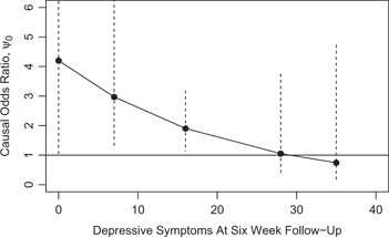
Causal odds ratio effect modified by depression levels at six week follow-up. The dotted lines represent 95 % confidence intervals. Point estimates calculated at the minimum, 25th percentile, median, 75th percentile, and 90th percentile on the depression scale distribution.

7 Discussion

We have used GSMMs to estimate causal effects that may be modified by potential intermediates and shown that our models can be equivalently expressed in terms of effect modification by observed posttreatment variables. Our work complements existing literature on noncompliance and mediation where conditioning also occurs on post-treatment variables. One natural comparison is to causal mediation analysis. It would appear that the analysis we have proposed differs substantially from the purpose of a causal mediation analysis. In mediation, the goal is to decompose a treatment effect into direct and indirect components [38]. The indirect treatment effect is an effect mediated by a third variable which transmits the treatment effect to the outcome. Mediation effects were of key interest in other analyses [2, 4]. In contrast, we stipulate only a total effect of the treatment that is conditional on levels of S. More specifically, we are only interested in how S alters effects, but we do not focus on any effect S has on Y. However, the identification conditions we invoke can, in another form, be used to identify mediation effects [39].

Our analysis has focused on a binary treatment. For treatments with more than two levels, the analysis may be extended by fitting a separate association model for each level of treatment, and defining H(ψ) for each subject by subtracting off the parametrized effect of the subjects’ observed treatment according to the proposed structural model. Restrictions on the effects of various treatment levels may be enforced through the parametrization of ψ in the blip down function from each treatment arm.

One weakness of this approach is its dependence on the specification of the association model. When the associated model is nonsaturated, it can be incompatible or uncongenial to the logistic SMM [40]. Vansteelandt et al. [41] argue that the biases from uncongenial estimators are small compared with other assumption failures. Moreover, alternatives are computationally demanding. Robust weights may be used to provide valid testing in the absence of treatment effects, but estimation of treatment effects may be subject to bias under the alternative. Moreover, in data analysis, nonconvergence was observed when baseline depression, a covariate that was highly predictive of the intermediate variable 6-week or 6-month depression, was omitted from the auxiliary model. The implication of this for practitioners is that model fitting of the association model should be completed carefully, with careful attention to functional form and the potential presence of interaction. Additional methodology to enhance robustness is one potential area for further research.

Identification of post-treatment effect modification may also be a useful tool in the development of “adaptive treatment strategies.” Under an adaptive treatment strategy, the treatment level and type are adjusted according to individual level characteristics [42, 43, 44, 45, 46, 47]. The design of adaptive treatment strategies requires choosing tailoring variables, variables that are used to decide how to adapt the treatment to specific individuals. Post-treatment effect modification provides one method for identification of tailoring variables. If the effect of a treatment varies across levels of a post-randomization variable, this would suggest that this covariate may be a good tailoring variable. Thus models where post-treatment covariates are allowed to modify causal effect estimates could be used for further actions within a study or to tailor clinical decision-making.

Funding statement: National Institute of Mental Health (Grant/Award Number: “RC4-MH-092722-01”).

Acknowledgments

For helpful comments and suggestions, we thank Stijn Vansteelandt, Eric Tchetgen Tchetgen, Teppei Yamamoto, the Associate Editor and the reviewers.

References

1. Vinokur A, Price R, Schul Y. Impact of the JOBS intervention on unemployed workers varying in risk for depression. Am J Community Psychol 1995;23:39–74.10.1007/978-1-4419-8646-7_22Search in Google Scholar

2. Imai K, Keele L, Tingley D. A general approach to causal mediation analysis. Psychol Methods 2010a;15:309–334.10.1037/a0020761Search in Google Scholar PubMed

3. Jo B. Causal inference in randomized experiments with mediational processes. Psychol Methods 2008;13:314–336.10.1037/a0014207Search in Google Scholar PubMed PubMed Central

4. Vinokur A, Schul Y. Mastery and inoculation against setbacks as active ingredients in the JOBS intervention for the unemployed. J Consult Clin Psychol 1997;65:867–877.10.1037/0022-006X.65.5.867Search in Google Scholar

5. Jo B, Vinokur A. Sensitivity analysis and bounding of causal effects with alternative identifying assumptions. J Educ Behav Stat 2011;36:415–440.10.3102/1076998610383985Search in Google Scholar PubMed PubMed Central

6. Little RJ, Yau LH. Statistical techniques for analyzing data from prevention trials: treatment of no-shows using Rubin’s causal model. Psychol Methods 1998;3:147–159.10.1037/1082-989X.3.2.147Search in Google Scholar

7. Mattei A, Li F, Mealli F, et al. Exploiting multiple outcomes in Bayesian principal stratification analysis with application to the evaluation of a job training program. Ann Appl Stat 2013;7:2336–2360.10.1214/13-AOAS674Search in Google Scholar

8. Angrist JD, Imbens GW, Rubin DB. Identification of causal effects using instrumental variables. J Am Stat Assoc 1996;91:444–455.10.3386/t0136Search in Google Scholar

9. Robins JM. Correcting for non-compliance in randomized trials using structural nested mean models. Commun Stat Theory Methods 1994;23:2379–2412.10.1080/03610929408831393Search in Google Scholar

10. Keele LJ. 2014. Conditioning on posttreatment quantities with structural mean models, Unpublished Manuscript.Search in Google Scholar

11. Rubin DB. Estimating causal effects of treatments in randomized and nonrandomized studies. J Educ Psychol 1974;6:688–701.10.1037/h0037350Search in Google Scholar

12. Rubin DB. Bayesian inference for causal effects: the role of randomization. Ann Stat 1978;6:34–58.10.1214/aos/1176344064Search in Google Scholar

13. Joffe MM, Small DS, Hsu C-Y. Defining and estimating intervention effects for groups that will develop an auxiliary outcome. Stat Sci 2007;22:74–97.10.1214/088342306000000655Search in Google Scholar

14. Vansteelandt S, Goetghebeur E. Causal inference with generalized structural mean models. J R Stat Soc Ser B 2003;65:817–835.10.1046/j.1369-7412.2003.00417.xSearch in Google Scholar

15. Dunn G, Bentall R. Modelling treatment-effect heterogeneity in randomized controlled trials of complex interventions (psychological treatments). Stat Med 2007;26:4719–4745.10.1002/sim.2891Search in Google Scholar PubMed

16. Vansteelandt S. Estimation of controlled direct effects on a dichotomous outcome using logistic structural direct effect models. Biometrika 2010;97:921–934.10.1093/biomet/asq053Search in Google Scholar

17. Vansteelandt S, Goetghebeur E. Using potential outcomes as predictors of treatment activity via strong structural mean models. Stat Sinica 2004;14:907–925.Search in Google Scholar

18. Rosenbaum PR. The consequences of adjusting for a concomitant variable that has been affected by the treatment. J R Stat Soc Ser A 1984;147:656–666.10.2307/2981697Search in Google Scholar

19. Frangakis CA, Rubin DB. Principal stratification in causal inference. Biometrics 2002;58:21–29.10.1111/j.0006-341X.2002.00021.xSearch in Google Scholar PubMed PubMed Central

20. Holland PW. Statistics and causal inference. J Am Stat Assoc 1986;81:945–960.10.1080/01621459.1986.10478354Search in Google Scholar

21. Neyman J. On the application of probability theory to agricultural experiments. Essay on principles. Section 9. Stat Sci 1923;5:465–472. Trans. Dorota M. Dabrowska and Terence P. Speed (1990).10.1214/ss/1177012031Search in Google Scholar

22. Rubin DB. Which ifs have causal answers. J Am Stat Assoc 1986;81:961–962.10.1080/01621459.1986.10478355Search in Google Scholar

23. Schwartz S, Gatto NM, Campbell UB. Extending the sufficient component cause model to describe the Stable Unit Treatment Value Assumption (SUTVA). Epidemiol Perspect Innovations 2012;9:1–11.10.1186/1742-5573-9-3Search in Google Scholar PubMed PubMed Central

24. Cuzick J, Sasieni P, Myles J, Tyrer J. Estimating the effect of treatment in a proportional hazards model in the presence of non-compliance and contamination. J R Stat Soc Ser B 2007;69:565–588.10.1111/j.1467-9868.2007.00600.xSearch in Google Scholar

25. Hernán MA, Robins JM. Instruments for causal inference: an epidemiologists dream. Epidemiology 2006;17:360–372.10.1097/01.ede.0000222409.00878.37Search in Google Scholar

26. Clarke PS, Windmeijer F. Identification of causal effects on binary outcomes using structural mean models. Biostatistics 2010;11:756–770.10.1920/wp.cem.2010.0210Search in Google Scholar

27. Robins JM, Rotnitzky A, Scharfstein D. Sensitivity analysis for selection bias and unmeasured confounding in missing data and causal inference models. In Halloran, E and Berry, D, editors. Statistical models in epidemiology: the environment and clinical trials. New York, NY: Springer, 1999:1–92.Search in Google Scholar

28. Follmann D. Augmented designs to assess immune response in vaccine trials. Biometrics 2006;62:1161–1169.10.1111/j.1541-0420.2006.00569.xSearch in Google Scholar

29. Robins JM. Non-response models for the analysis of non-monotone non-ignorable missing data. Stat Med 1997;16:21–37.10.1002/(SICI)1097-0258(19970115)16:1<21::AID-SIM470>3.0.CO;2-FSearch in Google Scholar

30. Robins J, Greenland S. Identifiability and exchangeability for direct and indirect effects. Epidemiology 1992;3:143–155.10.1097/00001648-199203000-00013Search in Google Scholar

31. Ten Have TR, Joffe M, Lynch KG, Brown GK, Maisto SA, Beck AT. Causal mediation analyses with rank preserving models. Biometrics 2007;63:926–934.10.1111/j.1541-0420.2007.00766.xSearch in Google Scholar

32. Mealli F, Mattei A. A refreshing account of principal stratification. Int J Biostat 2012;8:1–37.10.1515/1557-4679.1380Search in Google Scholar

33. Clarke PS, Windmeijer F. Instrumental variable estimators for binary outcomes. J Am Stat Assoc 2012;107:1638–1652.10.1080/01621459.2012.734171Search in Google Scholar

34. Hsu JY, Small DS. Discussion on “Dynamic treatment regimes: technical challenges and applications”. Electr J Stat 2014, Forthcoming.10.1214/14-EJS906Search in Google Scholar

35. Robins JM. Marginal structural models versus structural nested models as tools for causal inference. In Halloran, ME and Berry, D, editors. Statistical methods in epidemiology: the environment and clinical trials. New York, NY: Springer-Verlag, 1999:95134.10.1007/978-1-4612-1284-3_2Search in Google Scholar

36. Robins JMAR, Scharfstein D. Sensitivity analysis for selection bias and unmeasured confounding in missing data and causal inference models. In Halloran, ME and Berry, D, editors. Statistical models in epidemiology: the environment and clinical trials. New York, NY: Springer-Verlag, vol. 116, 1999:1–92.10.1007/978-1-4612-1284-3_1Search in Google Scholar

37. Franzese R, Kam C. Modeling and interpreting interactive hypotheses in regression analysis. Ann Arbor, MI: University of Michigan Press, 2009.Search in Google Scholar

38. Imai K, Keele L, Yamamoto T. Identification, inference, and sensitivity analysis for causal mediation effects. Stat Sci 2010b;25:51–71.10.1214/10-STS321Search in Google Scholar

39. Small DS. Mediation analysis without sequential ignorability: using baseline covariates interacted with random assignment as instrumental variables. J Stat Res 2011;46:91–103.Search in Google Scholar

40. Robins JM, Rotnitzky A. Estimation of treatment effects in randomised trials with non-compliance and a dichotomous outcome using structural mean models. Biometrika 2004;91:763–783.10.1093/biomet/91.4.763Search in Google Scholar

41. Vansteelandt S, Bowden J, Babanezhad M, Goetghebeur E. On instrumental variables estimation of causal odds ratios. Stat Sci 2011;26:403–422.10.1214/11-STS360Search in Google Scholar

42. Almirall D, Compton SN, Gunlicks-Stoessel M, Duan N, Murphy SA. Designing a pilot sequential multiple assignment randomized trial for developing an adaptive treatment strategy. Stat Med 2012;31:1887–1902.10.1002/sim.4512Search in Google Scholar PubMed PubMed Central

43. Collins LM, Murphy SA, Strecher V. The multiphase optimization strategy (MOST) and the sequential multiple assignment randomized trial (SMART): new methods for more potent eHealth interventions. Am J Preventive Med 2007;32:S112–S118.10.1016/j.amepre.2007.01.022Search in Google Scholar PubMed PubMed Central

44. Lavori P, Dawson R. A design for testing clinical strategies: biased adaptive within-subject randomization. J R Stat Soc Ser A 2000;163:29–38.10.1111/1467-985X.00154Search in Google Scholar

45. Murphy SA. Optimal dynamic treatment regimes. J R Stat Soc Ser B (Stat Methodol) 2003;65:331–355.10.1111/1467-9868.00389Search in Google Scholar

46. Murphy SM. An experimental design for the development of adaptive treatment strategies. Stat Med 2005;24:1455–1618.10.1002/sim.2022Search in Google Scholar PubMed

47. Robins JM. Optimal structural nested models for optimal sequential decisions. In Lin, D and Hagerty, P, editors. Proceedings of the second Seattle symposium in biostatistics. New York: Springer-Verlag, 2004:189–326.10.1007/978-1-4419-9076-1_11Search in Google Scholar

Published Online: 2016-7-28

Published in Print: 2016-9-1

This article is distributed under the terms of the Creative Commons Attribution Non-Commercial License, which permits unrestricted non-commercial use, distribution, and reproduction in any medium, provided the original work is properly cited.

Articles in the same Issue

https://doi.org/10.1515/jci-2015-0032

Keywords for this article

post-treatment interaction; structural mean model; causal odds-ratio

Creative Commons

BY-NC-ND 3.0