Robust Inferences from a Before-and-After Study with Multiple Unaffected Control Groups
-
Pengyuan Wang
 ,
Mikhail Traskin
,
Mikhail Traskin

Abstract
The before-and-after study with multiple unaffected control groups is widely applied to study treatment effects. The current methods usually assume that the control groups’ differences between the before and after periods, i.e. the group time effects, follow a normal distribution. However, there is usually no strong a priori evidence for the normality assumption, and there are not enough control groups to check the assumption. We propose to use a flexible skew-t distribution family to model group time effects, and consider a range of plausible skew-t distributions. Based on the skew-t distribution assumption, we propose a robust-t method to guarantee nominal significance level under a wide range of skew-t distributions, and hence make the inference robust to misspecification of the distribution of group time effects. We also propose a two-stage approach, which has lower power compared to the robust-t method, but provides an opportunity to conduct sensitivity analysis. Hence, the overall method of analysis is to use the robust-t method to test for the overall hypothesized range of shapes of group variation; if the test fails to reject, use the two-stage method to conduct a sensitivity analysis to see if there is a subset of group variation parameters for which we can be confident that there is a treatment effect. We apply the proposed methods to two datasets. One dataset is from the Current Population Survey (CPS) to study the impact of the Mariel Boatlift on Miami unemployment rates between 1979 and 1982.The other dataset contains the student enrollment and grade repeating data in West Germany in the 1960s with which we study the impact of the short school year in 1966–1967 on grade repeating rates.
1 Introduction
1.1 The before-and-after study with unaffected control groups for making causal inferences from an observational study: the Mariel Boatlift example
An observational study is an attempt to make causal inferences in a setting in which it is not feasible to randomly assign treatment to units. A major challenge for making causal inferences from observational study is that, because treatment is not randomized, the treatment and control groups may differ in ways other than the treatment. A “natural experiment” is an attempt to find a setting in the world where a treatment was handed to some people and denied to others for no particularly good reason that is haphazard [1, 2]. Good sources of natural experiments may be abrupt changes in government policies. As an example of a natural experiment from an abrupt change in government policy, we will consider Card’s [3] Mariel Boatlift study.
An important concern for immigration policy-makers is to what extent (if at all) do immigrants depress the labor market opportunities of native workers? A regression of native workers labor market opportunities (e.g., proportion employed or wages) on immigrant density in a city may yield a biased answer because immigrants tend to move to cities where the growth in demand for labor can accommodate their supply. Consequently, natural experiments, in which there are close to exogenous increases in the supply of immigrants to a particular labor market, are valuable for studying the effect of immigrants. Card [3] studied one such natural experiment, the experiences of the Miami labor market in the aftermath of the Mariel Boatlift.
Between April 15 and October 31, 1980, an influx of Cuban immigrants arrived in Miami, FL by boat from Cuba’s Mariel Harbor. Before this event there was a downturn in the Cuban economy which led to internal tensions, and subsequently the Cuban government announced that Cubans who wanted to leave could do so. By the end of the October, about 125,000 Cubans had arrived, at which point the Boatlift was ended by mutual agreement of the Cuban and U.S. governments. About half of the Cubans who arrived settled in Miami, thus significantly increasing the available labor force and number of Cuban workers in Miami.
We now discuss the before-and-after study with unaffected control groups study design for making causal inferences from the Mariel Boatlift study. In a causal inference study, a unit is an opportunity to apply or withhold treatment [4]. For the Mariel Boatlift study, we can think of the units as cities at a particular time, for example, Miami in 1979, Miami in 1982, Atlanta in 1979, Atlanta in 1982, etc. The Mariel Boatlift study can be thought of as a natural experiment that assigned some units to have a high amount of immigrants and some to have a low amount of immigrants, and where the outcomes of interest are labor market outcomes for native workers such as the unemployment rate. One way to study the effect of a high amount of immigrants would be to compare Miami after the Mariel Boatlift, say in 1982, to Miami before the Mariel Boatlift, say in 1979; this would be a before-and-after study. However, this study design may lead to biased results because the effect of the increase in immigration caused by the Mariel Boatlift may be confounded with macroeconomic changes between 1979 and 1982. In the before-and-after study with unaffected control groups, the change in outcomes in the place that got the treatment after a policy change or other event is compared to the change in outcomes in places that did not receive the treatment in either the before or after period, which are the unaffected control groups [2]; this is also sometimes called the difference-in-difference study design. The changes in the unaffected control groups control for changes in time, such as changes in the macroeconomy that would have occurred regardless of the treatment. Card [3] considered as unaffected control groups four other major cities in the United States – Atlanta, Houston, Los Angeles, and Tampa Bay–St. Petersburg. According to Card [3], these four cities did not experience a large increase in immigrants between 1979 and 1982 but were otherwise similar to Miami in demographics and pattern of economic growth. Consider the black unemployment rate as an outcome. The differences of blacks’ unemployment between 1979 and 1982 in Miami and the four unaffected control cities are shown in Figure 1.
The key assumption for the before-and-after study design with unaffected control groups to produce unbiased causal estimates is that the natural changes in the outcome that would have occurred in the group that received the treatment in the after period had that group not received treatment would have been the same as the change in the unaffected control groups [2]. This assumption is well discussed in the literature on treatments delivered to a group or cluster [5–7]. In the context of the Mariel Boatlift study, the key assumption is that the change in control cities like Atlanta or Houston serves as a counterfactual substitute and are exchangeable with the treated city, Miami.
In addition to needing this exchangeability assumption to hold, Figure 1 reveals an additional challenge: there is considerable variability among the changes in control groups, which suggests the possibility that the seemingly significant high difference of blacks’ unemployment rates in Miami may be just the result of random variation. To obtain valid causal inferences, we need to control for the natural variability among groups.
Differences of unemployment rates of blacks of 1979 and 1982 in five cities.
1.2 Current inference methods and the challenges
One way of making inferences that account for the variation in groups’ change in outcomes is a permutation approach [8]. The null hypothesis is that the unit to which the treatment was applied was randomly chosen and that the treatment has no effect. Consider the test statistic of the rank of the change between the before and after periods of the unit which was actually treated among all the units. Then, the p-value for testing the null hypothesis is the test statistic divided by the number of units. This permutation approach can work well if there are a large number of control groups, but it cannot find a significant effect, no matter how large the effect is, if there are only a few control groups. For example, if there is one treatment group and four control groups and the treatment group has the most extreme observation among all the groups, as in Figure 1, the permutation p-value is 1/5  0.2 no matter how large the treatment effect is.
Another nonparametric inference approach is the nonparametric bootstrap. Cameron et al. [9] proposed a series of nonparametric bootstrap approaches. However, we found in our simulation study (see Section 3) that when there is only one treatment group and four control groups, the bootstrap methods are not able to yield hypothesis tests with nominal significance levels.
As an alternative to non-parametric inference, we shall consider parametric models for the distribution of the control groups’ differences between the before and after periods, i.e. the group time effects. The most commonly used model is to assume that the groups’ differences between the before and after periods are i.i.d. normal random variables and to test whether the treatment group’s difference between the before and after periods could plausibly have come from the same distribution as the control groups [10]. This means that we conduct a t-test comparing the treatment group’s difference to the control groups’ differences. In the case where there are few treatment and control groups, the t-test is not protected by the central limit theorem and may be sensitive to the normal distribution assumption. From the simulation study in Section 3, the t-test actually performs well under non-normal distributed group variation but it is not totally robust, which means the rejection rate under null hypothesis may exceed its nominal significance level.
To make inferences more robust to violations of the normality assumption, we propose the robust-t method, a parametric method which considers a much wider range of distributions for the control groups’ differences. Specifically, we consider a set of skew-t distributions as in Jones and Faddy [11]. The family of skew-t distributions covers a wide range of shapes of distributions, and the normal distribution is a limiting case of the skew-t distribution. Our approach provides a researcher a method robust to a wide range of misspecification of the distribution of control groups’ differences between the before and after periods. We also propose a two-stage approach, which, compared to the robust-t method, has lower rejection rates under null hypothesis and lower power under alternative hypothesis, but provides an opportunity to conduct sensitivity analysis, and hence provides the researcher an idea about what kind of assumptions are necessary to reject the null hypothesis. Our overall proposal is to use the robust-t method to test for the overall range of shapes of group variation. If the test fails to reject, use the two-stage method to conduct a sensitivity analysis to see if there is a subset range of parameters for which we can be confident that there is a treatment effect.
The rest of the paper is organized as follows. In Section 2, we formulate the problem. In Section 3, we review some traditional methods and show the challenges with simulation. In Section 4, we develop the robust-t method, which is robust to a wide range of misspecification of the distribution of control groups’ differences between the before and after periods. In Section 5, we develop the two-stage method, which provides an opportunity to conduct sensitivity analysis. In Section 6, we compare the above two methods and propose to combine them when studying a real problems. In Sections 7 and Section 8, we apply the proposed methods to two examples. We conclude with discussion in Section 9.
2 Notation and model
2.1 Notation and model
In this paper, we consider groups of subjects and the outcomes are represented by the mean outcome of subjects of each group. Let
 be the average outcome of group k in period t assuming treatment was never applied to that group, and we model
 as
as
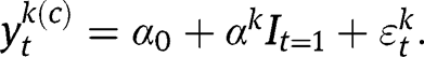
where
 indicates the period before and after the treatment,
 is the overall baseline level,
 is the time effect of group k, and
 ’s are independent normally distributed random errors with known standard deviation
 which signify the random measurement errors in our observations.
Let
 and
and
 represent the treatment and control groups, respectively. Letting
 be the average observed response for group k in period t, it follows
![[1]](/document/doi/10.1515/jci-2012-0010/asset/graphic/jci-2012-0010_eq1.png)
where
 is the causal effect of applying treatment in the groups k belonging to
 in the after period.
We assume that
 has the same distribution as
 . This means that we assume that the group(s) to which the treatment was applied was effectively randomly chosen. Presence of control groups allows us to separate the treatment effect
 from the time effect
 . If there is only one treatment and one control group, then it is common to assume time effects
 to be constant across groups, while if there are several treatment and/or control groups, the variation in the time effects can be taken into account by assuming that, for example,
 ’s follow a normal distribution with unknown variance. However, there is usually no strong a priori evidence for the normal distribution assumption.
In order to consider flexible group time effects,
 , we assume that
 are independently and identically distributed as a skew-
 distribution [11] with parameters
 controlling the skewness and scale, where
 is the nuisance scaling parameter.
The skew-t distribution is given by the following density function
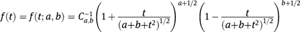
where
 ,
,
 denotes the beta function, and a and b are positive real numbers. When
 reduces to the density of the t-distribution with 2a degrees of freedom, and hence when
 and they are large, this distribution is similar to the normal distribution. When
 or
or
 is skewed to the left or right, respectively. The density functions of skew-t distributions with a range of parameters as well as the normal distribution are drawn in Figure 2, which shows that the skew-t distributions allow for flexibility in skewness and tail shapes.
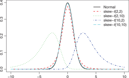
Density functions of skew-t and normal distributions.
The differences in observed outcomes between the before and after treatment periods are
![[2]](/document/doi/10.1515/jci-2012-0010/asset/graphic/jci-2012-0010_eq2.png)
2.2 Miami Boatlift effect study on Miami employment rates
The above structure could be applied to the Miami unemployment rates data to study the effect of the influx of immigrants on the unemployment rates. The dataset is from the Current Population Survey (CPS), which contains the employment status of people sampled between 1979 and 1982 from Miami and four other major cities which were considered to have similar employment situation to Miami. For each city in each time period, an unemployment rate
 was obtained from a complex survey, along with standard error of the estimator
 . Considering the size of the dataset, it is appropriate to assume that the estimated unemployment rate
 is the true unemployment rate with an error following
 distribution. We regard the unemployment rates as observations. Hence, there is one treatment group (Miami) and four control groups (the other four cities), and each group has one observation before and after the treatment period. Consider
 to be the unemployment rate in kth city in year 1979 (if
 ) or 1982 (if
 ) estimated from the survey, along with
 be the standard error of the estimator (see Section 7.3 for details). Let
 be indicator of Miami and
 be the indicators of the four unaffected cities. Letting
 and the Mariel Boatlift effect be denoted by
 the unemployment rates can be modeled by eq. [2] exactly.
We would like to view the massive immigration in the Mariel Boatlift as the “treatment” and know whether it increased the unemployment rates in Miami. The hypothesis test of interest is given by
![[3]](/document/doi/10.1515/jci-2012-0010/asset/graphic/jci-2012-0010_eq3.png)
Because there are only a small number of groups, it is not possible to estimate the parameters a and b of the skew-t distribution with any accuracy, so instead we consider a range of a and b’s which imply different skewnesses and tail shapes. We propose a robust-t method which guarantees nominal significance level across a wide range of plausible skew-t distributions and hence is robust to misspecification of the distribution of group time effects (Section 4). We also consider a two-stage method that has lower power than the robust-t method but provides an opportunity to infer the sensitivity with respect to specification of
 , and hence provides the researcher an idea about what kind of assumptions are necessary to reject the null hypothesis (Section 5). In the study of a real problem, we propose to use the robust-t method to test for the overall range of skew-t distributions of interest. If the test fails to reject, use the two-stage method to conduct a sensitivity analysis to see if there is a subset range of parameters for which we can be confident that there is a treatment effect.
We apply the proposed method to two datasets. One dataset is from CPS to study the impact of the Mariel Boatlift on Miami unemployment rates between 1979 and 1982. The other dataset contains the student enrollment and grade repeating data in West Germany in the 1960s to study the impact of the short school year 1966–1967 on the grade repeating rates. Both datasets have few control and treatment groups, and each group has only one observation before and after the treatment period.
3 Current methods: a simulation study
Several methods have been proposed for the hypothesis test (3), including bootstrap methods, t-statistic test, etc. Donald and Lang [10] made several basic points about the validity of the t-statistic test in various settings of the problems. Cameron et al. [9] summarized a series of bootstrap methods to test the treatment effect. It is well known that the bootstrap methods may not work well with small number of groups, and we confirm this point in our context with simulation.
According to the Miami unemployment rate dataset, we assume there is one treatment group and four control groups with one observation before and after the treatment period. We apply these methods to simulate datasets according to eq. [2] with given
 and
and
 for skew-t distribution, and show that they are not able to yield hypothesis tests with the nominal significance levels when there are few treatment and control groups and when group time effects are not normally distributed.
In Table 1, we list the 14 methods considered by Cameron et al. [9]. These methods are usually asymptotically efficient and work well with large number of treatment and control groups. A brief description of these methods can be found in Appendix A. More detailed description can be found in Cameron et al. [9]. Some of them are not applicable when there is one treatment group with one observation before and after the treatment period, as indicated in the “Applicable?” column.
We simulate datasets with one treatment group and four control groups according to eq. [2], where

 ,
,
 is the indicator of treatment group,
 are the indicators of control groups, and
 and
and
 for skew-t distribution are given. With
 and standard deviation of
 and
and
 to be 1 for
 the true rejection rates under a collection of the parameters
 ’s are listed in Table 8. The rejections rates and confidence interval lengths under more settings of the parameters
 can be found in Appendix A.
The results in Table 8 suggest that, in the situation with few treatment and control groups, the usual Wald tests are not able to yield hypothesis tests with the nominal significance level. The t-statistic test performs well with symmetric distributions, but becomes less robust with asymmetric distributions or one-sided tests. The cluster-robust method is supposed to perform well when the number of groups is large, but failed with the setting of few groups. The bootstrap methods are not able to yield hypothesis tests with the nominal significance levels as we expected, since they require large number of groups.
Some conventional methodsa.
| Method | Bootstrap? |  imposed? imposed? | Applicable? |
| Conventional Wald | |||
| 1. Default (iid errors) | No | – | Yes |
| 2. Moulton type | No | – | No |
| 3. Cluster-robust | No | – | Yes |
| 4. Cluster-robust CR3 | No | – | Yes |
| Wald bootstrap-se | |||
| 5. Pairs cluster | Yes | – | No |
| 6. Residuals cluster H0 | No | – | Yes |
| 7. Wild cluster H0 | Yes | – | Yes |
| BCA test | |||
| 8. Pairs cluster | Yes | No | |
| Wald bootstrap-t | |||
| 9. BDM | Yes | No | No |
| 10. Pairs cluster | Yes | No | No |
| 11. Pairs CR3 cluster | Yes | No | No |
| 12. Residuals cluster H0 | Yes | Yes | No |
| 13. Wild cluster H0 | Yes | Yes | Yes |
| 14. t-statistic | No | – | Yes |
Notes: [a]
4 Method 1: inference with robust-t method
The standard t-statistic test comparing the difference in the before-and-after differences between the treatment and control groups is commonly used in before-and-after studies. The test statistic is
 , where
 .
.
 .
.
 is the sample standard deviation of the treatment observations
 for
for
 , and
, and
 is the sample standard deviation of the control observations
 for
for
 .
.
If we assume that the t-statistic follows a t-distribution, this is the t-test. However, the t-distribution assumption is not valid without the normality assumption or protection from the central limit theorem with a large dataset. The simulation study in Section 3 shows that, the t-statistic test performs well with symmetric distributions, but becomes less robust with asymmetric distributions or one-sided tests.
In order to make the t-statistic robust to the distribution of group time effects deviating from the normal distribution, we assume that
 are independently and identically distributed as a skew-
 distribution [11]. For a given dataset, we specify a set of plausible parameters a and b’s for the skew-t distribution and the nuisance parameter
 . The idea is to use simulation to determine the cut-off values of the t-statistic to guarantee nominal significance level under this set of plausible parameters a, b and
 ’s. Hence, the hypothesis test with the cut-off values determined by simulation is robust to the distribution of group time effects deviating from normality over the considered range of parameters and hence we call it the robust-t method.
We use simulation to determine the cut-off values of the t-statistic by considering a wide range of parameters. To keep the simulation concise, we set the standard deviations of
 and
and
 to be
to be
 the same for all k. According to Proposition 2 (See Appendix C), scaling
 and
and
 simultaneously with the same scale factor would not change the rejection rates under the null hypothesis. We only need to consider a range of
 , rather than
 and
and
 separately, to determine the cut-off values of the t statistic in the robust-t method. In practice, when the standard deviations
  and
and
 differ, we just use the corresponding standard deviations of
 and
and
 in the simulation, and let
 ’s range be the maximum of
 across all possible k and t. We adjust the cut-off values of the t-statistic to guarantee the required significance level under the above settings of
 ,
,
 and
and
 . Suppose one wants to conduct the hypothesis test at significance level 0.05, the test procedure is summarized as below.
Specify a wide range of a and b to guarantee that they cover the plausible skew-t distributions.
To keep the simulation concise, we set the standard deviations of
 and
and
 to be
to be
 Specify a wide range of
 . When the standard deviations
 and
and
 differ, we just use the corresponding standard deviations of
 and
and
 in the simulation, and let
 ’s range be the maximum of
 across all possible k and t.
Under null hypothesis
 , simulate datasets according to model 2, obtain the t-statistics, and calculated the 0.025, 0.05, 0.95, 0.975 quantiles. (Note that if one wants to test with significance level other than 0.05, one just needs to modify the quantiles correspondingly.)
In order to let the robust-t method test have significance level 0.05 under all the above settings of
 and
and
 , we calculate the minimum of the 0.025,0.05 quantiles, and the maximum of 0.95,0.975 quantiles under the above settings. We use the minimum of 0.05 quantiles as the cut-off values of the left-sided test, the maximum of 0.95 quantiles as the cut-off value of the right-sided test, and minimum of 0.025 quantiles and maximum of 0.975 quantiles as the cut-off value of the two-sided test. This guarantees that the robust-t method test has significance level 0.05 under all the above settings of
 and
and
 .
.Test the hypothesis with the above specified cut-off values of the t-statistic.
In the above procedure, we adjust the cut-off values of the t statistic to guarantee nominal significance level across a wide range of skew-t distributions and
 . It only requires a vague range of the parameters
 and
and
 , and does not require specification of
 . Noting that we assume
 , rather than
 , is following skew-
 , the distribution of
 implied by the null hypothesis is properly centered at 0. Even if the skew-
 is extremely skew, the implied distribution of
 is symmetric. For example, it will always accept the null hypothesis if
 .
.
5 Method 2: two-stage inference and sensitivity analysis
The method in Section 4 is robust to misspecification of the random group time effect distribution since we adjust the cut-off values of the test statistic to guarantee nominal significance levels. If knowledge of
 of the skew-t distribution is available, another method overcoming the difficulty that
 is unknown is to conduct a two-stage inference.
5.1 Two-stage inference
For a given pair of
 we may use a simulation-based two-stage method to test hypothesis (3).
The two-stage inference is usually applied to hypothesis test with nuisance parameter(s) [12–14]. Generally, in a hypothesis test about
 with significance level
 with an unknown nuisance parameter
 the basic two-stage inference is conducted as follows.
Specify
 where
where
 .
.Derive a confidence interval
 of
of
 with coverage
 .
.For
 conduct the hypothesis test with significance level
 .
.If we accept the null hypothesis for
 we accept the null hypothesis. Then under null hypothesis, the false rejection rate is upper-bounded by
 .
.
In order to test the hypothesis (3), we follow the above two-stage inference procedure, where
 is the interval with the left end to be 0 and the right end to be
 upper bound of
 denoted by
 . One can prove that given larger
 , the null hypothesis is more likely to be rejected in the second stage. Thus in the second stage, we only need to test the null hypothesis with
 . The whole test procedure is summarized as follows.
Specify a range of plausible
 values.
Stage 1: For each pair of
 estimate an upper bound of
 with coverage
 with Monte Carlo simulation. The procedure to find the upper bound of
 is:
is:Set a tolerance error
 for the upper bound, for example, 0.001. Set sufficiently large number to be
 and 0 to be
 . Set k
 0 and
0 and
 .
.Use Monte Carlo simulation to estimate the distribution of the standard deviation of the control groups’ time effects with given
 and
and
 , and determine the empirical quantile (denoted by
 ) of the observed standard deviation of the control groups’ time effects.
If
 set
set
 . If
. If
 set k to be
 and return to step (b). If
 exit and use
 as the upper bound of
 .
.If
 set
set
 . If
. If
 set k to be
 and return to step (b). If
 exit and use
 as the upper bound of
 .
.
Stage 2: Denote the upper bound of
 to be
to be
 . Let the test statistic to be
 Compute the value
 of the test statistic T from the data. With
 and eq. [2] do the following:
Use Monte Carlo simulation to estimate the distribution of the test statistic T with
 .
.Either reject or accept
 depending on the empirical quantile of the observed test statistic value
 among the estimated distribution computed on the previous step, with significance level
 .
.
With the above two stage procedure, under null hypothesis the rejection rate would be upper-bounded by
 . Usually, the two-stage procedure is conservative, which means the rejection rate under the null hypothesis could be much smaller than
 .
.
The rejection rate under the null hypothesis depends on specific choice of
 and
and
 . We conducted a simulation study, and found that the choice of
 and
and
 has only slight influence on the rejection rate under the null hypothesis. In the rest of the paper, we set
 .
.
In Section 6, we compare the rejection rates under the null hypothesis and the powers under alternative hypothesis of the robust-t method and the two-stage method. We find that the power of this method is lower than the robust-t method proposed in Section 4.
5.2 Sensitivity analysis
When dealing with practical problems, usually some information about
 is available. For given
 assuming
 is known, one can conduct the hypothesis test
 as the second stage in the two-stage method. The test result may be heavily influenced by
 , and a sensitivity analysis can be conducted to find a subset of
 with which the null hypothesis is rejected.
Specifically, we set
 to range from low to high and investigate how the p-value of the hypothesis test
 changes along with
 . The procedure is summarized as follows:
Specify a range of plausible
 values.
For each pair of
 specify a range of
 ’s.
’s.For
 in the range considered, compute the value
 of the test statistic T from the data, calculated the p-value of the test, and see how the p-value would change with
 .
.
From the plot of
 ’s and the corresponding p-values, the method provides a researcher with an idea of what kinds of assumptions about the variation, skewness, and heavy-tailedness of the control groups’ differences would be necessary to infer that the treatment has an effect. See the applications in Sections 7 and 8.
6 Comparison and combination of the two approaches
With the robust-t method, one has to specify a plausible range of the parameters
 and
and
 . In many of the cases, it is not difficult to make the range large enough to guarantee to cover the range of parameters of interest. For example, in the study of mass immigration effect on Miami unemployment rates, observations are proportions, and hence differences before and after the treatment period should be within
 . It implies that
 could not be too large. Also,
 can be set to arrange from small to large (which represents heavy-tailed to thin-tailed), and from
 to
to
 or
or
 (which represents symmetry to heavy asymmetry) to cover the shape of the distribution of group time effects. The robust-t method is robust to a wide range of misspecification of
 . We set uniform cut-off values for the test for all the
 within the range of interest, and guarantee required significance level.
Also, the robust-t method has higher power than the two-stage method, even if the two-stage method specifies the right
 . We compare the rejection rates and powers of the two methods with simulation as in Appendix B. The simulation results show that, under a wide range of parameters, the power of the robust-t method is larger than that of the two-stage method, even if the two-stage method specifies the right
 . The advantages of the robust-t method suggest that we use the robust-t method to conduct the hypothesis test for the overall range of
 of interest in the before-and-after study when there are few control and/or treatment groups.
However, the two-stage method provides an opportunity to conduct the sensitivity analysis as in Section 5.2 to find out a possible subset of parameters where the null hypothesis can be rejected. In the study of a real problem, we propose to use the robust-t method to conduct the hypothesis test for the overall range of parameters of interest. If the test fails to reject, use the two-stage method to do a sensitivity analysis to see if there is a subset range of
 and
and
 for which we can be confident that there is a treatment effect.
7 Application one: Mariel Boatlift effect on Miami employment rates
7.1 Dataset and problem
Between April 15 and October 31, 1980, an influx of Cuban immigrants arrived in Miami, Florida by boat from Cuba’s Mariel Harbor. In order to study the effect of mass immigration on unemployment rates, we obtained the CPS data of 1979 and 1982 in Miami and four other cities: Atlanta, Houston, Los Angeles, and Tampa Bay–St. Petersburg, which did not experience a large increase in immigrants between 1979 and 1982 but, according to Card [3], were otherwise similar to Miami in demographics and pattern of economic growth. The dataset contained a “race” variable which divided subjects in “white,” “black,” and “other.” The dataset also contained an “ethnic” variable which divided subjects into “Mexican American,” “Chicano,” “Mexicano,” “Puerto Rican,” “Cuban,” “Central or South American,” “Other Spanish,” “All other,” and “Don’t know.” All the non-hispanics except unknowns were labeled as “All other.” Within the dataset we get, all people labeled as “Cuban” were labeled as “white” in terms of race.
Table 2 and Figure 3 show the unemployment rates in 1979 (before the Boatlift) and 1982 (after the Boatlift) in Miami and four control cities. Figure 4 shows the increment of the unemployment rates from 1979 to 1982. All of the cities experienced increase in unemployment between 1979 and 1982, but Miami experienced a larger increase, particularly among blacks. Is there strong evidence that Miami experienced a larger increase in unemployment than could be expected if the immigration had no effect? The effect of the immigration to Miami is confounded with the downturn in the economy between 1979 and 1982. Therefore, we control for time by comparing the difference of unemployment rates between the before and after periods in Miami to those of the unaffected cities.
Average unemployment rates of treatment and control cities in 1979 and 1982.
| 1979 | 1982 | |
| Miami | ||
| General unemployment rate | 0.059 | 0.097 |
| Whites without Hispanics unemployment rate | 0.045 | 0.050 |
| Blacks without Hispanics unemployment rate | 0.086 | 0.160 |
| Hispanics unemployment rate | 0.055 | 0.083 |
| Control cities | ||
| General unemployment rate | 0.056 | 0.083 |
| Whites without Hispanics unemployment rate | 0.046 | 0.067 |
| Blacks without Hispanics unemployment rate | 0.100 | 0.130 |
| Hispanics unemployment rate | 0.047 | 0.073 |
Unemployment rates of 1979 and 1982 in the five cities.
Differences of unemployment rates of 1979 and 1982 in the five cities.
Since the treatment effect is the same for all the individuals sampled in Miami and the city time effect is the same for all individuals sampled in the corresponding city, by aggregating the individual employment status to unemployment rates we would not lose the information about the city time effects and treatment effect. Also because of the complex sampling method in the CPS, the usual assumption that the observations are independent is not plausible for this dataset. Hence, for this dataset, for each city in each time period, an unemployment rate was obtained from the complex survey, along with the standard error of the estimators (see Section 7.2 for details). We regard the unemployment rates as the observations, and hence there is one treatment group (Miami) and four control groups (the other four cities), and each group has one observation before and after the treatment period. The years 1979 and 1982 correspond to the time period before and after the migration, respectively.
We would like to know whether the massive immigration in the Mariel Boatlift had an increasing effect on the unemployment rates in Miami. Let
 be the estimated unemployment rate in the kth city in year 1979 (if
 ) or 1982 (if
 ). Let
 be indicator of Miami and
 be the indicators of the four unaffected cities. The standard error of the estimation is estimated with binomial approximation corrected by a sampling strategy factor provided by CPS. Considering the size of the dataset, it is appropriate to assume that the estimated
 is the true unemployment rate with an error following
 distribution, where
 is the estimated standard error of estimated
 . Letting
 and the Mariel Boatlift effect denoted by
 the unemployment rate data can be models by eq. [2]. The hypothesis test of interest is given by
![[4]](/document/doi/10.1515/jci-2012-0010/asset/graphic/jci-2012-0010_eq4.png)
We test the hypothesis with the unemployment rates of four different groups: the unemployment rate of the population, the unemployment rate of whites without Hispanics, the unemployment rate of blacks without Hispanics, and the unemployment rate of Hispanics.
7.2 Data and setup
We obtain
 and
and
 as follows.
We estimated the unemployment rate
 by the ratio of number of unemployed sampled individuals and available labor force in the dataset. We use the variable “ftpt79 (Full-time or part-time labor force status)” as the indicator of employment condition. The value of this variable includes: not in labor force (0), employed full-time (1), part-time for economic reasons (2), unemployed full-time (3), employed part-time (4), and unemployed part-time (5). We estimate the unemployment rate by the ratio of the number of individuals with value (3) and (5) to the number of individuals with value values (1), (2), (3), (4) or (5).
 is estimated as the standard error of estimated
 . For each city k at time t, let x be the number of unemployed people and y be the labor force, we have
 . The CPS calculate the standard error of
 by
by
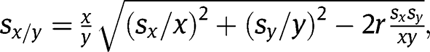
where r is the correlation between x and y. According to the U.S. Bureau of Census (2000), the analyst should assume r is equal to zero [15]. For each city k at time t, let n be the total number of observations, we calculate
and
where
 are the design effect coefficients on standard errors. We use the design effects for total monthly variances after composing on Unemployment and Civilian Labor Force as Table 14–5 in CPS [15, Chapter 14]. For each city in each time period, we calculate
 ,
,
 and obtain
 as the standard error of unemployment rate. The estimated standard error of city k at time t are treated as the standard deviation of the error terms
 , for
, for
 and
and
7.3 Robust-t test of the mass migration effect
7.3.1 The cut-off values under 1 control and 4 treatment groups
Corresponding to the Miami unemployment dataset, we consider one treatment group and four control groups with mean outcome in each group before and after the treatment period. Let
 range from 2 to 160,
 and
and
 range from 2–10 to 210. Hence, our test is robust to a wide range of
 the scaling factor of the skew-t distribution, and to a wide range of parameters
 for the skew-t distribution changing from seriously skewed to symmetric, from heavy-tailed to thin-tailed. Using the simulation procedure specified in Section 4, the cut-off values for the robust-t method which should be used in hypothesis test are estimated as in Table 3.
Cut-off values for 1 control and 4 treatment groups.
| Quantile | Cut-off value |
| 0.025 | –6.29 |
| 0.05 | –4.08 |
| 0.95 | 4.08 |
| 0.975 | 6.29 |
Using the computed cut-off values, the rejection rates under null hypothesis with datasets generated with skew-t distributed group time effects range from 0.004 to 0.018, according to different  we use to generate the datasets.
7.3.2 Hypothesis test results with robust-t method
We apply the cut-off values to conduct the hypothesis test (4) with the unemployment rates of four different groups: the unemployment rate of the population, the unemployment rate of whites without Hispanics, the unemployment rate of blacks without Hispanics, and the unemployment rate of Hispanics. In 1979, there were very few Hispanics in Atlanta and the unemployment rate of Hispanics in Atlanta was zero, and hence the estimated standard error was zero. We could either set the corresponding error term to be 0, or delete the city Atlanta from the dataset when testing the effect of the mass migration on the unemployment rate of Hispanics. We test the Boatlift effect on the unemployment rate of Hispanics with these two settings separately.
The result is that we accept the null hypothesis that the Mariel Boatlift did not affect the unemployment rate for any of the groups of people we studies.
We also conducted a two-sided test and the confidence intervals of the unemployment rates of groups of people are reported in Table 4.
Confidence intervals of unemployment rates using robust-t method.
| Group | ||||
| General | Whites | Blacks | Hispanics | Hispanicsa |
| (–0.027,0.048) | (–0.041, 0.007) | (–0.048,0.144) | (–0.015,0.005) | (–0.015,0.004) |
Notes: [a]
From the robustness point of view, we accept the null hypothesis with group time effects following a range of distributions with various shapes, and hence the hypothesis testing is robust to misspecification of the distribution of group time effects.
7.4 Sensitivity analysis
Since the robust-t approach fails to reject the null hypothesis, we use the two-stage method to do a sensitivity analysis as in Section 5.2 to see if there is a subset range of parameters for which we can be confident that there is a treatment effect.
We set
 to be various values and look at how the p-value of the hypothesis test
 changes along with the
 . As an example, we summarize the results with Blacks’ unemployment rate with a small collection of
 ’s in Figure 5. The graph implies that, even with
 , the treatment effect is not statistically significant because of the variation in the estimated unemployment rates, and hence there is not significant evident to conclude that the migration affects the Blacks’ unemployment rates.
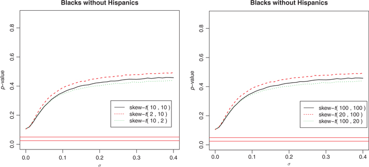
p-value changes with
 for blacks.
The height of the horizontal line is 0.025 and 0.05 respectively.
8 Application two: short school year effect on German school grade repeating rates
We study the effect of the length of the school year on student performance with a student enrollment dataset of West Germany in the 1960s. After the Second World War, all the states of West Germany (Federal Republic of Germany) except Bavaria, started school year in spring. To diminish the frictions with other parts of Europe, the prime ministers reached an agreement on the unification of the school system in 1964. According to this agreement the start of the school year would be moved to the end of summer. This change was conducted by the beginning of the 1967 school year, and thus most of the states experienced a short school year in 1966–1967. The influence of the short school year on the grade one to four repeating rates was analyzed in Pischke [16]. We apply our proposed methods to this dataset to test whether the short school year increased grade-repeating rates.
8.1 Dataset and problem
The number of students enrolled in each grade and the number of students repeating the corresponding grade was published annually by the Federal Statistical Office in the serial Fachserie A. Bevölkerung und Kultur, Reihe 10, I, Allgemeines Bildungswesen. Our dataset contains the numbers of students and repeating students in grade one to four in the eleven states of West Germany from the year 1961–1971. In 1965, all the West German states had a normal long school year, while in 1966, some of the states experienced a short school year in order to fulfill the requirement of the agreement by the beginning of the 1967 school year. We view this short school year in 1966–1967 as the “treatment” to the states, and would like to study the influence of short school year on grade repeating rates, assuming state time effects following skew-t distribution.
Among the eleven states, Schleswig-Holstein, Bremen, Nordrhein-Westphalen, Hessen, Rheinland-Pfalz, Baden-Württemberg and Saarland experienced short school year in 1966–1967, and hence they were the treatment states. Hamburg, Bayern and Berlin stuck to a regular long school year, and thus they were the control states. Niedersachsen adopted the short school years in 1966, but added additional time in subsequent years for some schools, so it was neither purely treatment nor control group, and we decided not to consider this state in this study.
We summarize the average grade repeating rates of treatment and control states in 1965 and 1966 in Table 5 and draw them in Figure 6. They suggest that the short school year may have increased the grade repeating rates. The differences of the grade repeating rates of year 1966 and 1965 in Figure 7 show the same implication.
With the model (2) described in Section 2, we study the short school year effect on each grade with aggregate grade repeating rates in 1965 and 1966. There are seven treatment groups and three control groups. For each grade let
 be the grade repeating rate in kth state in year 1965 (if
 ) or 1966 (if
 ), which is estimated by the ratio of the number of students repeating a grade and the number of students enrolled in the corresponding grade.
 is the standard error of the corresponding grade repeating rate, which is estimated by binomial approximation. Let
 be the indicators of the seven treatment states (Schleswig-Holstein, Bremen, Nordrhein-Westphalen, Hessen, Rheinland-Pfalz, Baden-Württemberg and Saarland) and
 be the indicators of the three unaffected states (Hamburg, Bayern and Berlin). The short school year effect is represented by
 and the hypothesis test of interest is

Average grade repeating rates of treatment and control states in 1965 and 1966.
| 1965 | 1966 | |
| Treatment states | ||
| Grade one repeating rate | 0.043 | 0.042 |
| Grade two repeating rate | 0.046 | 0.053 |
| Grade three repeating rate | 0.038 | 0.040 |
| Grade four repeating rate | 0.034 | 0.035 |
| Control cities | ||
| Grade one repeating rate | 0.042 | 0.04 |
| Grade two repeating rate | 0.044 | 0.041 |
| Grade three repeating rate | 0.034 | 0.034 |
| Grade four repeating rate | 0.032 | 0.029 |
Grade repeating rates of 1965 and 1966 in the ten states.
Differences of grade repeating rates of 1965 and 1966 in the ten states.
8.2 Robust-t test of the short school year effect
8.2.1 The cut-off values under 3 control and 7 treatment groups
Letting
 ranging from 2 to 160,
 , and
, and
 ranging from 2–10 to 210, using to the simulation procedure specified in Section 4, the cut-off values which should be used in hypothesis test are estimated as in Table 6.
Cut-off values for 3 control and 7 treatment groups.
| Quantile | Cut-off value |
| 0.025 | –2.53 |
| 0.05 | –2.03 |
| 0.95 | 2.03 |
| 0.975 | 2.53 |
Using the computed cut-off values, the rejection rates under null hypothesis with datasets generated with skew-t distributed group time effects range from 0.0015 to 0.033, according to different
 we use to generate the datasets.
8.2.2 Hypothesis test results with robust-t method
The result is that we accept the null hypothesis that the short school year did not affect the repeating rates of the grades we studied.
We also conducted a two-sided test, and the 95% confidence intervals of the repeating rates of each grade are reported in Table 7.
Confidence intervals of grade repeating rates using robust-t method.
| Grade 1 | Grade 2 | Grade 3 | Grade 4 |
| (–0.023,0.026) | (–0.00079, 0.020) | (–0.015,0.018) | (–0.014,0.021) |
8.3 Sensitivity analysis
We use the two-stage method to do a sensitivity analysis as in Section 5.2 to see if there is a subset range of parameters for which we can be confident that there is a treatment effect. We again set
 to be various value and look at how the p-value of the hypothesis test
 changes along with the
 . As an example, we summarize the results with the grade 2 repeating rate with a small collection of
 ’s in Figure 8. The graph implies that, one has to assume that
 is small to conclude that the short school year affects the grade 2 repeating rate. Typically
 needs to be smaller than 0.005 for the collection of
 ’s we tested.
In the two-stage estimation process, we estimate the 0.975 upper bound of
 in stage 1. For the collection of
 ’s we test and the grade 2 repeating rate data, the 0.975 upper bounds of
 varies from 0.002 to 0.01, which is not large comparing to the 0.005 threshold. If one assumes
 to be smaller than 0.005, it may be concluded that the short school year affects the grade 2 repeating rate.
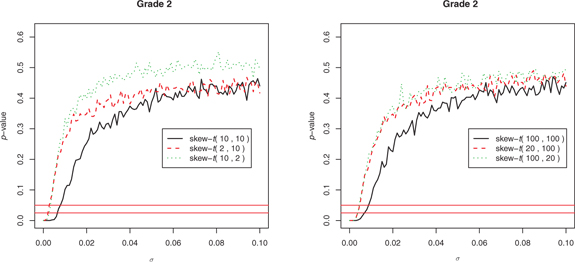
p-value changes with
 for grade 2 repeating rate.
The height of the horizontal line is 0.025 and 0.05 respectively.
9 Conclusion and discussion
The before-and-after study usually assumes that group time effects follow a normal distribution. There is usually no strong a priori evidence for the normality assumption. When there are a large number of groups, the normality assumption can be checked. But if there are only a small number of groups, it is difficult to check the normality assumption. In this paper, we propose the robust-t method using a flexible skew-t distribution to model group time effects, and consider a range of plausible skew-t distributions to make the method robust to misspecification of distribution of group time effects. We also propose a two-stage approach, which has lower power, but provides an opportunity to infer the sensitivity with respect to specification of
 , the variation parameter of group time effects. In the study of a real problem, we propose to use the robust-t method to test for the overall range of shapes of group variation. If the test fails to reject, use the two-stage method to conduct a sensitivity analysis to see if there is a subset range of parameters for which we can be confident that there is a treatment effect. In a study with only one control group such as Card and Krueger [17], such a sensitivity analysis is the only option – the effect of treatment is completely confounded with the group time effects. The choice of a, b and
 is arbitrary but one should make the range broad enough to cover the situation (skewness, fat-tailedness, scale, etc.) of the dataset under research.
The family of skew-t distributions is a generalization of the t-distribution, and the shape can range from heavy-tailed to thin-tailed, asymmetric to symmetric. Note that our method can work with any family of distributions, as long as we can draw samples from it. Thus, the method is generalizable and can incorporate other distributions to model the group time effects.
Appendix A: more simulation results of bootstrap and t-statistic methods with few treatment and control groups and time effects not normally distributed
A description of methods
We apply the Wald test and bootstrap methods to the simulated datasets generated according to eq. [2]. The details of the methods can be found in Cameron et al. [9], and we describe them roughly as follows.
The Wald test has several sub-methods. The conventional Wald test assumes independently and identically distributed errors and applies ordinary least square (OLS) estimators. If there exist cluster errors, the estimated variances of coefficients are biased. One approach to correcting this bias is to use Moulton-type standard errors. In random effect model, cluster–robust Wald test applies cluster–robust variance estimator instead of the variance estimator in OLS. The cluster–robust variance estimator is modified by a correction proposed by Bell and McCaffrey [18]. This correction generalizes the HC3 measure (jackknife) of MacKinnon and White [19], and is referred to as the CR3 variance estimator by Cameron et al. [9]. Another way of correction called bias-corrected accelerated (BCA) procedure is defined in Efron [20], and Hall [21].
The bootstrap procedure may use the bootstrap estimates of coefficients to form the bootstrap estimates of standard errors, which are referred to as Wald bootstrap-se methods by Cameron et al. [9]. Or it may use the bootstrap estimates of t-statistic to form the bootstrap estimates of quantiles of t-statistic, which are referred to as Wald bootstrap-t methods by Cameron et al. [9].
The bootstrap strategy may resample the clusters with replacement from the original samples and form the “pairs cluster” bootstrap method. The CR3 correction may be applied when estimating the t-statistic, which forms the “pairs CR3 cluster” bootstrap method. Bertrand et al. [22] applies a pairs cluster bootstrap using the bootstrap-t procedure, but with default OLS standard errors, rather than cluster-robust standard errors, and it forms the “BDM” bootstrap method.
Resampling the residuals and constructing new values of the dependent variable forms the “residuals cluster” bootstrap methods. The “wild cluster” resamples the residuals but the signs are changed to the opposite randomly with probability 0.5.
Corresponding to the unemployment rate dataset, we assume one treatment group and four control groups, with mean outcome for each group before and after the treatment period. In such setting, some of the above-mentioned methods are not applicable because of singularity issues.
One way to construct the Moulton-type standard error in random effect model is to use the estimated cluster-specific random effects and individual i.i.d errors. This approach (method 2) may not be applied to our setting of the problems, since there is only one observation in each group and one cannot estimate individual errors.
The pairs cluster bootstrap methods (method 5, 8, 9, 10, and 11) may not be applied to our problem, since it is very possible to sample the same set of independent variables in a run of bootstrap and hence results in infinitely large Wald statistic.
The bootstrap method which resamples residuals with the null hypothesis imposed (method 12) may not be applied to our problem, since it may generate a bootstrap dataset with dependent variable perfectly fitted by the independent variables, which produces an infinitely large value of the Wald statistic.
Complemental simulation results
We simulate datasets with one treatment group and four control groups according to eq. (20), where
 ,
,
 is the indicator of treatment group,
 are the indicators of control groups, and
 and
and
 for skew-t distribution are given. With
 and standard deviation of
 and
and
 to be 1 for
 , besides Table 8 in Section 3, the true rejection rates and confidence interval lengths for
 under more settings of
 are listed in Tables 9, 10 and 11.
The results in both Tables 8 and 9 suggest that, in the situation with few treatment and control groups, the usual Wald tests are not able to yield hypothesis tests with their nominal significance level. The t-statistic test performs well with symmetric distributions, but becomes less robust with asymmetric distributions or one-sided tests. The cluster-robust method is supposed to perform well when the number of groups is large, but failed with the setting of few groups. The bootstrap methods are not able to yield hypothesis tests with the nominal significance levels as we expected, since they require large number of groups.
Rejection rate of some methods.
| Parameters (a,b) for skew-t distribution | |||||
| (2,3) | (3,2) | (2,10) | (10,2) | (50,2) | |
| 1. Default (iid errors) | 0.164 | 0.167 | 0.115 | 0.166 | 0.146 |
| 3. Cluster-robust | 0.504 | 0.530 | 0.510 | 0.483 | 0.476 |
| 4. Cluster-robust CR3 | 0.475 | 0.476 | 0.466 | 0.445 | 0.441 |
| 6. Residuals cluster H0 | 0.058 | 0.060 | 0.043 | 0.054 | 0.062 |
| 6. Residuals cluster H0 Left | 0.086 | 0.093 | 0.077 | 0.086 | 0.084 |
| 6. Residuals cluster H0 Right | 0.083 | 0.084 | 0.059 | 0.087 | 0.101 |
| 7. Wild cluster H0 | 0.000 | 0.000 | 0.000 | 0.000 | 0.000 |
| 13. Wild cluster H0 | 0.460 | 0.488 | 0.418 | 0.457 | 0.456 |
| 14. t-statistic | 0.050 | 0.054 | 0.041 | 0.062 | 0.066 |
| 14. t-statistic left | 0.054 | 0.060 | 0.045 | 0.059 | 0.032 |
| 14. t-statistic right | 0.057 | 0.047 | 0.030 | 0.052 | 0.078 |
Rejection rate of some methods (continued).
| Parameters (a,b) for skew-t distribution | |||||
| (10,15) | (15,10) | (3,3) | (15,15) | (100,100) | |
| 1. Default (iid errors) | 0.134 | 0.126 | 0.138 | 0.145 | 0.187 |
| 3. Cluster-robust | 0.505 | 0.489 | 0.522 | 0.492 | 0.517 |
| 4. Cluster-robust CR3 | 0.461 | 0.442 | 0.482 | 0.436 | 0.493 |
| 6. Residuals cluster H0 | 0.041 | 0.047 | 0.056 | 0.055 | 0.068 |
| 6. Residuals cluster H0 Left | 0.068 | 0.075 | 0.084 | 0.088 | 0.105 |
| 6. Residuals cluster H0 Right | 0.077 | 0.067 | 0.068 | 0.068 | 0.087 |
| 7. Wild cluster H0 | 0.000 | 0.000 | 0.000 | 0.000 | 0.000 |
| 13. Wild cluster H0 | 0.458 | 0.442 | 0.462 | 0.455 | 0.498 |
| 14. t-statistic | 0.044 | 0.049 | 0.050 | 0.052 | 0.068 |
| 14. t-statistic left | 0.044 | 0.043 | 0.052 | 0.054 | 0.066 |
| 14. t-statistic right | 0.043 | 0.046 | 0.044 | 0.046 | 0.060 |
Appendix B: comparison of the two methods
Corresponding to the Miami unemployment rate dataset, we assume one treatment group and four control groups with mean outcome in each group before and after the treatment period. We also considered the case with seven treatment groups and three control groups, corresponding to the dataset described in Section 8 and the results were similar. Again to keep the simulation concise, we set the standard deviation of
 and
and
 to be
to be
 the same for all
 . We assume that
 range from 2 to 160,
 and
and
 ranges from 2–10 to 210.
CI length of some methods.
| Parameters (a,b) for skew-t distribution | |||||
| (2,3) | (3,2) | (2,10) | (10,2) | (50,2) | |
| 1. Default (iid errors) | 5.79 | 5.84 | 6.27 | 6.09 | 10.71 |
| 3. Cluster-robust | 2.24 | 2.26 | 2.43 | 2.36 | 4.15 |
| 4. Cluster-robust CR3 | 2.51 | 2.53 | 2.72 | 2.64 | 4.64 |
| 6. Residuals cluster H0 | 5.27 | 5.39 | 5.66 | 5.59 | 9.87 |
| 7. Wild cluster H0 | 4.94 | 5.18 | 5.20 | 5.20 | 9.10 |
| 13. Wild cluster H0 | 3.07 | 3.18 | 3.34 | 3.24 | 5.46 |
| 14. t-statistic | 9.39 | 9.49 | 10.18 | 9.89 | 17.39 |
CI length of some methods (continued).
| Parameters (a,b) for skew-t distribution | |||||
| (10,15) | (15,10) | (3,3) | (15,15) | (100,100) | |
| 1. Default (iid errors) | 5.74 | 5.84 | 5.76 | 5.86 | 5.74 |
| 3. Cluster-robust | 2.29 | 2.26 | 2.23 | 2.27 | 2.22 |
| 4. Cluster-robust CR3 | 2.56 | 2.53 | 2.50 | 2.54 | 2.48 |
| 6. Residuals cluster H0 | 5.37 | 5.28 | 5.23 | 5.30 | 5.35 |
| 7. Wild cluster H0 | 4.94 | 4.86 | 4.96 | 4.91 | 5.20 |
| 13. Wild cluster H0 | 3.02 | 3.05 | 3.12 | 3.13 | 3.15 |
| 14. t-statistic | 9.61 | 9.48 | 9.36 | 9.52 | 9.32 |
Under the above range of parameters, we compare the rejection rates under the null hypothesis and the powers under the alternative hypothesis of the two methods we proposed in Sections 4 and 5 with simulation and show that, under such range of parameters, the power of the robust-t method is larger than that of the two-stage method, even if the two-stage method specifies the right
 .
.
Rejection rates under null hypothesis
Let
 range from 2 to 160. Scaling
 and
and
 simultaneously with the same scale factor would not change the rejection rates under the null hypothesis, according to the proposition 1 (Appendix D). We only need to consider a range of
 , rather than
 and
and
 separately, to investigate the rejection rates under null hypothesis in various settings. So we let
 and
and
 range from 2–10 to 210. Using the simulation procedure specified in Section 4, the cut-off values for the robust-t method which should be used in hypothesis test are estimated as in Table 3.
Using the computed cut-off values, the rejection rates under null hypothesis with datasets generated with skew-t distributed group time effects range from 0.004 to 0.018, according to different
 we used to generate the datasets.
We also investigate the rejection rates under null hypothesis of the two-stage procedure. Again we set the standard deviations of
 and
and
 to be
to be
 the same for all k.
Under the considered range of parameters, the rejection rates of the two-stage method are no larger than 0.002, which is obviously inferior to the robust-t method. Thus the robust-t method has higher rejection rate under null hypothesis.
Powers under alternative hypothesis
Again we use the cut-off values computed in Table 3 in Section 4 to conduct the hypothesis test with robust-t method. We investigate the power of the two-stage procedure.
Letting the proportion of the true
 and
and
 range from 1 to 100, and the ratio of
 and
and
 be 1, we summarize the powers of the two methods for some combinations of
 in Figure 9. With other settings of
 and the ratio of
 and
and
 , the results are similar. The figures show that, in general the robust-t method has larger power than the two-stage method.
The power of the two-stage method basically stays at 0 when the skew-t distribution is very skewed. The reason is that, for a given dataset, we estimate the p-value by generating datasets with assumed skew-t parameters, computing the statistics T’s from the generated datasets, and then compare the statistic
 from the given dataset to the statistics T’s from the generated datasets. However, when the skew-t distribution is very skewed, the statistics T’s from the generated datasets can be very spread out, and hence result in insignificant p-value even when the true
 is large.
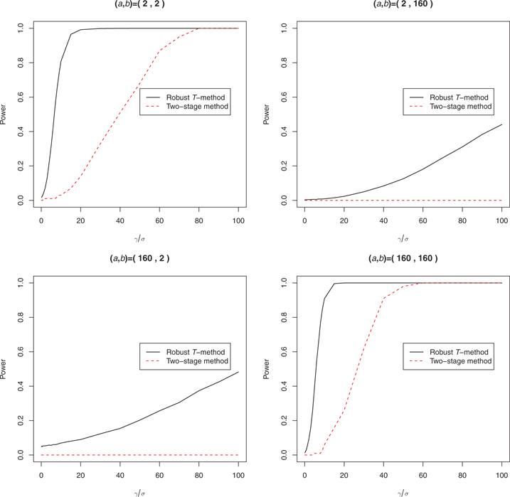
Comparison of the powers of the two methods, 1 treatments and 4 controls.
In order to check the robustness of the method, we also applied the robust-t method to non-skew-t distributions such as uniform distribution and Gamma distribution. Typical results are shown in Figure 10. For comparison we also draw the power under skew-t distribution with
 on each of the plot. The rejection rates under null hypothesis (which is the power when
 ) and the power under gamma and uniform distribution are close to the skew-t distribution, which shows the robustness of the method against misspecification.
Under the Gamma distribution, the rejection rates under null hypothesis is below 0.05. Under the uniform distribution it is slightly above 0.05, but is still reasonably controlled. The reason that the method performs slightly worse under the uniform distribution is that this distribution is flat in its supporting area, and hence makes it harder for the robust-t method to precisely determine the center, and hence the horizontal position of the true distribution.
Appendix C: Proposition 1
Proposition 1: Given
 of the skew-t distribution, consider two models. The first model follows eq. [2] with
 skew-
skew-
 , and
, and
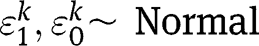
 while the second model follows eq. [2] with
 skew-
skew-
 , and
, and
 . Conducting the robust-t method inference for the treatment effect with data following the two models, the rejection rates under the null hypothesis
 are identical.
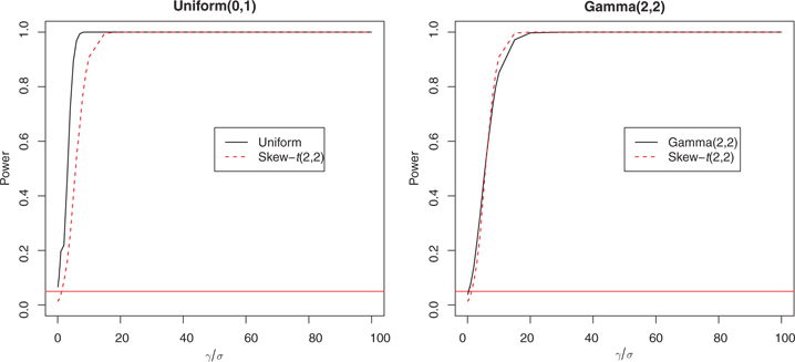
Power under other distributions, 1 treatments and 4 controls.
The height of the horizontal line is 0.05.
This proposition shows that scaling
 and
and
 simultaneously with the same scale factor would not change the rejection rates under the null hypothesis. Thus we only need to consider a range of
 , rather than
 and
and
 separately, to determine the cut-off values of the t statistic in the robust-t method.
Proof. Suppose that a dataset
 follows the first model, it has
![[5]](/document/doi/10.1515/jci-2012-0010/asset/graphic/jci-2012-0010_eq5.png)
where
 skew-
skew-
 ,
,

 is the set of the indicators of treatment groups and
 is the set of the indicators of control groups.
Under null hypothesis,
![[6]](/document/doi/10.1515/jci-2012-0010/asset/graphic/jci-2012-0010_eq6.png)
If we scale
 ,
,
 and
and
 simultaneously by factor
 the model becomes
![[7]](/document/doi/10.1515/jci-2012-0010/asset/graphic/jci-2012-0010_eq7.png)
Letting

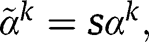
 and
and
 then
then
 skew-
skew-
 and
and  . Hence, the dataset
 follows the second model.
Considering the robust-t method inferences for the two datasets, it is obvious that if we accept the null hypothesis for the first dataset, we accept the null hypothesis for the second dataset and vice versa. Hence, the rejection rates under null hypothesis are identical for the two models. Proof completed.∎
Appendix D: Proposition 2
Proposition 2: Given
 of the
 -t distribution, consider two models. The first model follows eq. [2] with
 skew-
skew-
 , and
, and
 while the second model follows eq. [2] with
 skew-
skew-
 , and
, and
 . Conducting the two-stage inference for the treatment effect with data following the two models, the rejection rates under the null hypothesis
 are identical.
This proposition means that scaling
 and
and
 simultaneously with the same scale factor would not change the rejection rates under the null hypothesis. Thus we only need to consider a range of
 , rather than
 and
and
 separately, to find the rejection rates under the null hypothesis.
Proof. Suppose that a dataset
 follows the first model, it has
![[8]](/document/doi/10.1515/jci-2012-0010/asset/graphic/jci-2012-0010_eq8.png)
where
 skew-
skew-
 ,
,

 is the set of the indicators of treatment groups and
 is the set of the indicators of control groups.
Under null hypothesis,
![[9]](/document/doi/10.1515/jci-2012-0010/asset/graphic/jci-2012-0010_eq9.png)
If we scale
 ,
,
 and
and
 simultaneously by factor
 the model becomes
![[10]](/document/doi/10.1515/jci-2012-0010/asset/graphic/jci-2012-0010_eq10.png)
Letting

 and
and
 then
then
 skew-
skew-
 and
and
 . Hence, the dataset
 follows the second model.
Consider the two-stage inferences for the two datasets. In the first stage, letting the upper bound of
 to be
to be
 for the first dataset and
 for the second, then obviously
 . In the second stage, letting the test statistic to be
 for the first dataset and
 for the second dataset, then under null hypothesis
 . Thus these two test statistics would have identical quantiles among the distributions of test statistic generated by
 and
and  correspondingly. Thus, if we accept the null hypothesis for the first dataset, we accept the null hypothesis for the second dataset and vice versa. Hence, the rejection rates under null hypothesis are identical for the two models. Proof completed.▪
References
1. Rosebaum P. Design of observational studies. New York: Springer, 2009.10.1007/978-1-4419-1213-8_3Search in Google Scholar
2. Meyer BD. Natural and quasi-experiments in economics. J Bus Econ Stat 1995;13:151–61.Search in Google Scholar
3. Card D. The impact of the mariel boatlift on the miami labor market. Ind Labor Relations Rev 1990;43:245–57.10.1177/001979399004300205Search in Google Scholar
4. Rosebaum P. Observational studies, 2nd ed. New York: Springer, 2002.10.1007/978-1-4757-3692-2Search in Google Scholar
5. Murray D. Design and analysis of group-randomized trials, vol. 29. New York: Oxford University Press, 1998.Search in Google Scholar
6. Murray D, Hannan P, Wolfinger R, Baker W, Dwyer J. Analysis of data from group-randomized trials with repeat observations on the same groups. Stat Med 1998;17:1581–600.10.1002/(SICI)1097-0258(19980730)17:14<1581::AID-SIM864>3.0.CO;2-NSearch in Google Scholar
7. Murray D, Varnell S, Blitstein J. Design and analysis of group-randomized trials: a review of recent methodological developments. Am J Public Health 2004;94:423–32.10.2105/AJPH.94.3.423Search in Google Scholar
8. Abadie A, Diamond A, Hainmueller J. Synthetic control methods for comparative case studies: estimating the effect of California’s tobacco control program. J Am Stat Assoc 2010;105:493–505.10.1198/jasa.2009.ap08746Search in Google Scholar
9. Cameron CA, Miller D, Gelbach JB. A bootstrap-based improvements for inference with clustered errors. Rev Econ Stat 2008;90:414–27.10.1162/rest.90.3.414Search in Google Scholar
10. Donald SG, Lang K. Inference with difference-in-differences and other panel data. Rev Econ Stat 2007;89:221–33.10.1162/rest.89.2.221Search in Google Scholar
11. Jones MC, Faddy MJ. A skew extension of the t-distribution, with applications. J Roy Stat Soc, Ser B (Methodological) 2003;65:159–74.10.1111/1467-9868.00378Search in Google Scholar
12. Pagan A. Two stage and related estimators and their applications. Rev Econ Stud 1986;53:517–38.10.2307/2297604Search in Google Scholar
13. Proschan M. Two-stage sample size re-estimation based on a nuisance parameter: a review. J Biopharm Stat 2005;15:559–74.10.1081/BIP-200062852Search in Google Scholar
14. Zhao L, Lipsitz S. Designs and analysis of two-stage studies. Stat Med 2006;11:769–82.10.1002/sim.4780110608Search in Google Scholar
15. CPS. Design and methodology. Technical Paper 63RV, 2002.Search in Google Scholar
16. Pischke J-S. The impact of length of the school year on student performance and earnings: evidence from the German short school years. Econ J 2007;117:1216–42.10.1111/j.1468-0297.2007.02080.xSearch in Google Scholar
17. Card D, Krueger A. Minimum wages and employment: a case study of the fast food industry in New Jersey and Pennsylvania, 1993.10.3386/w4509Search in Google Scholar
18. Bell R, McCaffrey D. Bias reduction in standard errors for linear regression with multi-stage samples. Surv Methodol 2002;28:169–82.Search in Google Scholar
19. MacKinnon J, White H. Some heteroskedasticity-consistent covariance matrix estimators with improved finite sample properties. J Econometrics 1985;29:305–25.10.1016/0304-4076(85)90158-7Search in Google Scholar
20. Efron B. Better bootstrap confidence intervals. J Am Stat Assoc 1987;82:171–85.10.1080/01621459.1987.10478410Search in Google Scholar
21. Hall P. The bootstrap and Edgeworth expansion. New York: Springer Verlag, 1997.Search in Google Scholar
22. Bertrand M, Duflo E, Mullainathan S. How much should we trust differences-in-differences estimates? Q J Econ 2004;119:249–75.10.1162/003355304772839588Search in Google Scholar
©2013 by Walter de Gruyter Berlin / Boston
Articles in the same Issue
- Masthead
- Masthead
- Targeted Data Adaptive Estimation of the Causal Dose–Response Curve
- Analysis of Subgroup Data of Clinical Trials
- Robust Inferences from a Before-and-After Study with Multiple Unaffected Control Groups
- Targeted Minimum Loss-Based Estimation of Causal Effects in Right-Censored Survival Data with Time-Dependent Covariates: Warfarin, Stroke, and Death in Atrial Fibrillation
- Causal, Casual and Curious
- The Curse of Free-Will and the Paradox of Inevitable Regret