Evaluation of mobile mapping point clouds in the context of height difference estimation

1.1 Motivation

In recent years the usage of 3D point clouds captured by mobile mapping systems (MMS) or other sources has become more popular due to technological advances and the related increase in interest from different fields of applications [1]. The main advantages of MMS are their efficient data acquisition and versatile applicability, as different platforms exist for different application areas on land, water, and in the air. Compared to terrestrial laser scanning (TLS) point clouds, the uncertainty is assumed to be higher because the system’s pose has to be known for every timestamp to geo-reference every measured point. Deviations from the pose estimation coming from the used navigation sensors like global navigation satellite systems (GNSS) or inertial measurement units (IMUs) influence the uncertainty of the point cloud.

For many applications, the uncertainty of the extracted parameters from the point cloud data has to be known since this is essential information for the customer to interpret them. For example in the case of deformation monitoring of retaining walls [2], the uncertainty of the points on the wall has to be known in order to interpret the computed displacements from MMS measurements correctly. Parameters that are often wanted are, for example, the position and orientation of objects or their geometrical properties, like shape or size. However, to derive the uncertainty of these parameters is a difficult task for mobile mapping systems, since multiple error sources influence the quality of the point cloud like the previously mentioned navigation sensors.

To estimate the uncertainty of the extracted parameters, two different approaches can be considered. The first one is called forward modeling. By modeling the uncertainty of every used sensor of the system and their functional relation on the point cloud or the parameter, the uncertainty of the latter can be derived. This can be achieved for example by variance propagation [3], 4] or Monte Carlo simulation [5], [6], [7], [8] as suggested in the Guide to the Expression of Uncertainty in Measurements (GUM) [9]. In [10], a forward modeling approach is performed and the resulting theoretical position uncertainties are compared with an empirical plane-based approach. The authors showed, that the position uncertainty derived empirically and theoretically are similar in their test environments. The main assumptions are, that no remaining systematic errors from the components of the system and no GNSS multipath or signal loss are present. This assumption does not hold especially in urban areas.

The major drawback of these approaches is, that the uncertainty distribution of the used sensors is unknown. In many cases, especially for commercial systems, this prior knowledge is unavailable. Furthermore, the sensor fusion for the pose estimation and the point cloud generation is often performed within commercial software, where the exact functional relationship is not accessible. Additionally, the correlations are often neglected in these approaches, since the computational effort would be enormous to compute and store a covariance matrix of the whole point cloud. The size of this matrix would be 3n _pts × 3n _pts , where n _pts represents the number of points in the point cloud. However, the information about the correlations between points is necessary for a correct estimation of the uncertainty of the derived parameters. In [10] the authors only derive the position uncertainty but ignore correlations between neighboring points. For the evaluation of the uncertainty of relative parameters like height differences, this information is missing.

The second approach is called backward modeling. Unlike the first approach, the uncertainty of the extracted parameters is derived empirically without modeling any input uncertainties. Therefore these parameters are extracted from captured point cloud data and are compared against reference data. The also called ground truth data should be at least one magnitude more accurate than the expected uncertainty of the system [11]. In this work, we follow the backward modeling approach.

The considered parameters in recent works using empirical approaches are evaluated using different features or methods. The absolute position or height uncertainty is evaluated using distinct points. These points are realized by artificial targets [12], [13], [14], [15] or point features like building corners or centers of poles [13]. Additionally, point-to-plane distances to reference planes are used to evaluate the absolute position of planar objects [10], 16]. By using the distances coming from cloud comparisons, the position of objects can be evaluated, that are not planar. One frequently used method is the Multiscale Model to Model Cloud Comparison (M3C2) [17]. The idea is to compare the captured point cloud with a reference point cloud without a parameterization of the scanned object. The main advantage is, that no assumptions about the geometric properties of the objects have to be made. Furthermore, the comparison provides dense information on the deviations between both point clouds over the scanned area. In [18] a kinematic laser scanning system is evaluated by comparing the measured point cloud with a reference captured with a laser tracker. The aim was to evaluate the performance of the pose estimation of the system. The main disadvantage of cloud comparisons is, that in-plane displacements can not be detected [19].

Besides the position, distances between objects are also evaluated. In [20] the performance of an indoor mobile mapping system is evaluated by analyzing the distances between targets with different distances and angles. Others evaluate the uncertainty of the extracted geometric properties, like the radius of a cylindric object [4].

The previous works mainly focus on the uncertainty of the absolute position of objects as a parameter to describe the uncertainty of the point cloud data. For many applications, however, this parameter is not important. The evaluation of MMS point cloud data should be linked to the actual application fields, where the system can be used.

Since, to the best of our knowledge, only the absolute height uncertainty was considered, in this paper we analyze the uncertainty of height differences in point clouds. The relative height difference between objects is relevant in the field of ground subsidence monitoring, where discontinuities in the height situation of the surface may occur, which can result in damage to structures [21]. Another application field is the deformation monitoring of engineering buildings, like bridges [22]. Potential tilts of these structures are analyzed by computing height differences between two points at the two sides of the bridge, which are measured by leveling. By considering the distance between both points, an inclination can be derived.

To evaluate the uncertainty of height differences properly, three key questions are tackled in this work, which might influence the uncertainty and which can change considering the application:

1. How does the uncertainty of the height difference depend on the traveled distance between two height observations? Due to the estimation of a smooth trajectory and the usage of sensors like GNSS and IMUs, the pose information is highly correlated between neighboring time stamps. Because of this, we assume that points, which are measured shortly after each other, are also highly correlated. This causes a change in the height difference uncertainty concerning the traveled distance or more precisely the time gap between the acquisition of both objects.

2. How do the environmental conditions impact the uncertainty of height differences? The trajectory estimation process usually relies on GNSS positioning, which is influenced by the surroundings of the master and rover antenna. Bad GNSS conditions indicated by a small number of visible satellites or a high PDOP (Positional Dilution of Precision) value [23] lead to inaccurate pose estimation, which influences the height information and consequently also the height difference information.

3. How does the location of the objects relative to the measuring system influence the uncertainty of the height differences between them? Due to uncertainties in the system calibration [12] and other factors the point uncertainty may vary depending on the location of the object relative to the scanning system. Consequently, the uncertainty of height differences between a pair of points will also be influenced.

For the evaluation of the height difference uncertainty the captured road surface is used, where the MMS is driving on. The major advantage is, that the height information of the road surface is almost always available. Consequently, we can easily evaluate the uncertainty of height differences for different traveled distances and environmental conditions. The three questions will be tackled as follows: In Section 2 the basic concept and the used data sets are presented. Additionally, the procedure of how to derive and analyze the height difference information from the point cloud data will be explained in this section. In Section 3 the conducted experiments and the results are shown and discussed. The findings are summarized in Section 4 and used to answer the three key questions.

2.1 Data collection

In this part, the used mobile mapping system and the two captured data sets in different environments are presented.

2.1.1 Measurement system

The measurement system used in this work is shown in Figure 1. For the navigation task, an inertial navigation system iMAR iNAV-FJI-LSURV (https://www.imar-navigation.de/en/) with fiber optic gyroscopes, servo accelerometers, and RTK-GNSS (Real Time Kinematic) is used. The IMU has a random walk error of below 0.001 deg / h and 8 μg for the angular rate and the acceleration. According to the manufacturer, the true heading information is better than 0.01 deg and the attitude is better than 0.002 deg while using RTK-GNSS. The position uncertainty is specified as 2 cm while using RTK-GNSS. The trajectory estimation is performed in the software Waypoint Inertial Explorer 8.90 and 9.00 [25]. Depending on the GNSS quality, accuracies of centimeters and a hundredth of a degree or better can be reached for the position and orientation according to the manufacturer. For the mapping task, a 2D laser scanner Z + F Profiler 9012A is mounted on the system [26]. The precision is specified as 0.2–0.5 mm at a distance of 10 m depending on the reflection properties of the measured surface. The maximum profile rate is 200 Hz and the maximum scan rate is 1,016 kHz. The external calibration is done by a plane-based approach described in [12]. The authors showed, that the uncertainty of the lever arm is below 0.5 mm and for the boresight angles below 0.002 deg using all realizations from multiple measurements. The calibration measurements were conducted in the summer of 2019. Consequently, the computed calibration parameters are more than 4 years older than the considered point cloud data in this publication. The platform for the system is either a trolley or, in our case, a van. A case study on a motorway showed that the uncertainty of the absolute height is about a few millimeters to one cm under good GNSS conditions [27].

Figure 1:

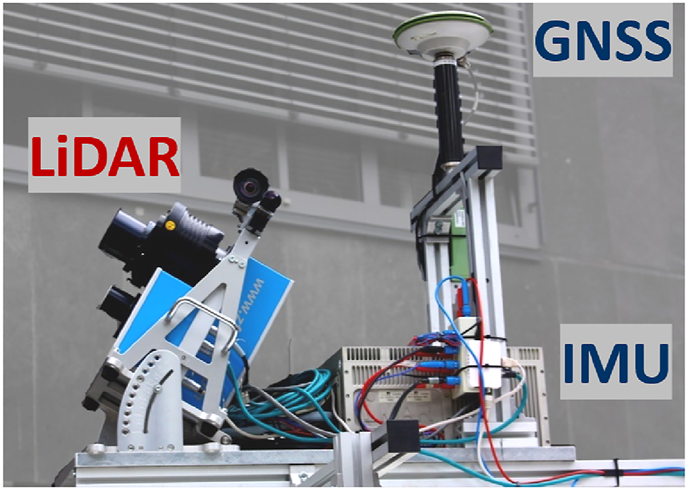
Used mobile mapping system. Left: Z + F Profiler 9012A profile laser scanner; Right: iMAR iNAV-FJI-LSURV IMU and RTK GNSS antenna.

2.1.2 Public road data set

The first data set was captured on a public road near Cologne, Germany. Figure 2 shows the considered road part. The two-lane road part is around 3 km long and has an approximate height change of 30 m. The entire road section leads through a forest so GNSS conditions are expected to be bad. Figure 3 shows the environmental conditions on the road from the cockpit of a car. The trees near the road occlude the sky, so that the GNSS signals are blocked or disturbed. The measurement starts at the northern town “Bensberg” and after driving over the reference road part, the system turns to the southern town “Forsbach” and drives back to “Bensberg”. This procedure was performed 5 times so that the number of acquisitions of the road surface is 10. The average speed was around 70 km/h for the highlighted road part in every pass. The elapsed time between the first and the last pass of the road is approximately 2 h.

Figure 2:

Considered public road part between Bensberg and Forsbach (Source: www.tim-online.nrw.de/tim-online2/).

Figure 3:

Environmental conditions inside the forest in the public road data set.

For the RTK-GNSS solution, we use a virtual reference station computed by SAPOS NRW. The coordinate of the reference station is chosen in the center of the test environment, such that the maximum baseline is under 2 km. We expect no additional errors coming from the length of the baseline.

2.1.3 Rural dataset

The second data set is captured in a rural area at the outdoor laboratories of the agricultural faculty of the University of Bonn on Campus Klein-Altendorf, Germany. The chosen road part displayed in Figure 4 is approximately 1.8 km long. It connects the northern and the southern parts of the campus. In the near surroundings of the road are just a few buildings and mostly fields, so the GNSS conditions are assumed to be very good at every spot. Consequently, the absolute height information is expected to be precise within the expected margin of a few centimeters over the whole test site. The road is measured with the MMS 14 times (seven forward and backward passes) in total within 1 h and 40 min. The driving speed was nearly constant at approximately 30 km/h.

Figure 4:

Overview of the test site and the placed artificial targets. The bottom map shows the distribution of the target locations in the test site. The upper figure shows the distances of the targets relative to the road center. Negative values denote, that the target is located on the left side of the road while driving from south to north.

Additionally, 13 artificial targets are placed along the road at different distances to the road center (see Figure 4) to analyze the impact of the location of the height measurement relative to the mobile mapping system. The distances to the road center are visualized by the upper part of the figure. Targets with a negative distance to the road center are located on the left while driving from south to north. Most targets are placed directly next to the road surface, so they have a distance of about 2.5 m. Some targets are further away from the road center, like point B26 with a distance of about 9 m. The used planar targets have an eight-fold pattern and are presented in [28]. The generation of their reference heights and height differences is explained in Section 2.1.4.

As for the public road data set, we use a virtual reference station computed by SAPOS NRW for the RTK-GNSS solution at the center of the test environment.

2.1.4 Generation of reference data

To evaluate the trueness of height differences derived by the mobile mapping point cloud, we need reference data that is at least one magnitude better than the expected uncertainty of the height difference information of the used system [11]. For the public road data set (see Section 2.1.2), no reference data is available. Consequently, only the precision can be analyzed. For the rural data set presented in Section 2.1.3, the coordinates of the artificial targets use an existing reference point network with uncertainty in the lower mm range [12]. Targets, which are not placed on points of the reference network are determined using a Leica MS60 multi-station from multiple viewpoints from the network. The uncertainty of the height differences coming from the network adjustment software is better than 5 mm, which is around half a magnitude superior to the expected uncertainty from the mobile mapping system. Depending on the distance between the targets, the uncertainty decreases to below 1 mm. The 2D location of every target center is given in UTM, whereas the height information represents physical heights. Please note, that the MMS can only measure ellipsoidal heights. Physical heights and height differences are not equal to the ellipsoidal ones. To tackle this problem, the undulation model German Combined Quasigeoid (GCG2016) [29] is used. The physical heights of the target are transformed to ellipsoidal heights so that we can evaluate the trueness of the system properly. The absolute accuracy of the model is for this region around 1–2 cm, but the relative accuracy is expected to be higher. Nevertheless, the usage of the GCG2016 can cause systematic errors in the estimated physical height differences of the MMS concerning the spatial distance. The reason is a deviation regarding the undulation variation of the model at the test area.

Besides the reference coordinates of the artificial targets, we scanned one part of the road surface with the Leica MS60 multi-station. The area is shown in Figure 5. The MS60 is placed on point P5 and further network points are used to fix the orientation. The scanning function of the multi-station is used to capture a geo-referenced point cloud of the marked area. The scanned points are used to derive reference cross fall information at the grid points, which lie within the scanned region. We assume, that systematic deviations coming from bad incident angles and the surface properties of the road do not severely influence the uncertainty of the derived cross fall. Alternatively, geometric leveling in the small area could also serve as more reference data, which is more accurate.

Figure 5:

Region of the scanned road with the Leica MS60.

2.2 Extraction of height difference information

To evaluate the height difference information, we first need to extract height information at different locations from the point cloud. In this work, we primarily use the scanned road surface to obtain this information. We extract two different parameters here, which tackle different influencing factors of the height difference uncertainty: height information of the road surface along the road axis and the road cross fall, which describes the inclination of the road surface perpendicular to the road axis. As seen in the motivation, height differences are often used to describe the inclination of an object. In this case, we use the derived cross fall uncertainty to describe the uncertainty of height differences at a certain distance across the road axis. We distinguish between the two height differences because the first one describes the distance dependency and the other evaluates the influence of the location relative to the system. As an additional source for both factors, we use artificial targets to evaluate height differences at different locations.

2.2.2 Estimation of heights and height differences

In this part, we present how to extract the height difference information for all of the three used sources.

2.2.2.1 Height differences from grid points along the road axis

The point cloud points X _c are given in global-cartesian coordinates, in this case in the coordinate frame ETRS89, since the mobile mapping system uses GNSS observations for positioning. To derive height information out of the point cloud data, the points are firstly transformed to ellipsoidal coordinates and afterward to UTM coordinates [30]. By doing this we ensure, that ellipsoidal height is represented by the z-axis and the x- and y-axis defining the 2D location. The same transformation is performed for the grid points X grid ( i ) and the road axis points in A r .

At every grid point location, the neighboring point cloud points are extracted, by checking if the 2D distance to the grid point location is below a radius r (see Figure 6):

(2) ( x c − x grid ( i ) ) 2 + ( y c − y grid ( i ) ) 2 ≤ r , i = 0 , … , n

Figure 6:

Grid points X grid ( i ) along the road axis and buffer with radius r for point extraction.

We set the value for r to 0.5 m for both data sets. By doing this, we ensure, that no point in the point cloud is used for the height determination for multiple grid points. Additionally, enough points are extracted in both data sets to ensure a robust height estimation. Especially for the public road data set, the velocity of 70 km/h causes a rather low point density with a gap of around 0.1 m between the scanning profiles.

The filtered points X i n ( i ) are reduced by its corresponding grid point X grid ( i ) :

(3) X red ( i ) = X i n ( i ) − X grid ( i ) .

The reduced points X red ( i ) are used to estimate a plane (see equation (4)).

(4) n x ⋅ x red ( i ) + n y ⋅ y red ( i ) + n z ⋅ z red ( i ) − d = 0

The resulting plane parameters n x n y n z T and d are used to determine the relative height between the road surface and the corresponding grid point x grid ( i ) y grid ( i ) T . To do this, we evaluate the plane equation at x red ( i ) = y red ( i ) = 0 , which represents the 2D location of the grid point in the reduced coordinate system. We compute the relative height δh⁽ⁱ⁾ at the location of the grid point X grid ( i ) by dividing the distance parameter d by the z-component of the normal vector n _z :

(5) δ h ( i ) = d n z .

The height determination is illustrated in Figure 7. Please note, that for the absolute height information, we have to add the initial ellipsoidal height z grid ( i ) of the grid point since we reduced the points by its coordinates (see equation (3)).

(6) h ( i ) = z grid ( i ) + δ h ( i )

Figure 7:

Height estimation process using plane estimation for every grid point with points lying in the buffer with radius r.

It should be pointed out, that the surface representation can be changed to more complex ones like B-Splines if needed.

The height difference u^(i,j) between two grid points is obtained by subtracting the height values h⁽ⁱ⁾ and h^(j) from each other.

(7) u ( i , j ) = h ( j ) − h ( i )

Figure 8 visualizes the height difference between two grid points on the road surface.

Figure 8:

Height profile of a road and height difference between two grid points X grid ( 4 ) and X grid ( 7 ) lying on the road axis.

2.2.2.2 Height differences from road cross fall

Since the location of the road axis relative to the mobile mapping systems stays nearly the same, additional information is needed to determine the entire uncertainty of height differences. To overcome this problem the cross fall of the road is computed at each grid point X grid ( i ) , which describes the inclination of the road perpendicular to the road axis at this location. Since inclinations are also described by height differences (see Section 1), the opposite can be performed if a scale is given by a distance. The idea is, to use all point cloud points lying on the considered cross-profile to determine the inclination instead of estimating the height value at the center and the side of the road and computing a difference. To do this, the profile points at the grid point X grid ( i ) have to be extracted first. Therefore, we first need to extract the points lying on the road surface from the rest of the point cloud. There are several methods to automatically detect the road in point clouds [31], 32]. In this paper, we extracted the road surface manually. To extract the cross-profile and derive the cross fall from a 2D-line fit at the grid point X grid ( i ) , we need to transform the points, such that the x-axis is parallel to the road axis. Therefore we use the previously used UTM coordinates and ellipsoidal heights X _c of the point cloud, where the y-axis points to the north pole. First, we extract the neighboring points using equation (2). The radius r is chosen here to 10 m so that we guarantee, that the full cross-profile is inside this radius. Afterwards, we reduce the points according to equation (3) using the current grid point X grid ( i ) .

Then we rotate the points around the z-axis and afterward around the rotated y-axis (see equation (8)). By doing this, we ensure that the cross-section lies in the YZ-plane, which is oriented perpendicular to the road axis. The transformation is visualized in Figure 9.

(8) X R A ( i ) = R y β R z α X red ( i )

Figure 9:

Transformations into road axis frame: first step: rotation around the z-axis with angle α (left); second step: rotation around the rotated y-axis (right).

The angles α and β are computed from the transformed road axis points P a UTM ( k ) and P a UTM ( k + 1 ) (see (1)).

(9) α = arctan ⁡ 2 x a UTM ( k + 1 ) − x a UTM ( k ) y a UTM ( k + 1 ) − y a UTM ( k )

(10) β = arcsin z a ′ ( k + 1 ) − z a ′ ( k ) ‖ P a ′ ( k + 1 ) − P a ′ ( k ) ‖

The axis points P a ′ ( k ) are received by rotating them with R z α .

Only the points lying in a buffer along the road axis with a certain width δ around the grid position X grid ( i ) are used for the estimation process:

(11) x R A ( i ) − δ 2 ≤ 0 ≤ x R A ( i ) + δ 2 .

Please note that the coordinates of the points are reduced by the values of the grid point X grid ( i ) in equation (3). The value for δ is chosen to 0.5 m for both data sets for the same reasons as the search radius r before. Especially because of the point density the buffer has to have a certain size, such that multiple profiles of the laser scanner are extracted for the computation. We assume, that the cross fall does not change within this buffer.

Usually, the cross fall is estimated for every road lane independently. In both considered data sets, we distinguish between two lanes, which we both capture in each pass. Since the origin of the transformed coordinate system is the road axis, which is located in the center of the road, we can distinguish between both lanes by the sign of the y-coordinate y R A ( i ) .

(12) X left ( i ) = X R A ( i ) y R A ( i ) > 0

(13) X right ( i ) = X R A ( i ) y R A ( i ) < 0

In the following, we name the sides of the road left and right. As we can see in equations (12) and (13), the left side is where the y-coordinates are positive, and the right side, where the y-component is negative for the remaining points within the buffer. Since the underlying coordinate system is defined independently from the trajectory information, the right lane is the same side of the road for forward and backward passes, although the vehicle changed lanes. As a result, we only consider the same lane for the evaluation at once and do not mix them together, because we assume that the cross fall is not the same on both sides of the road. In both data sets the road course goes from south to north and the set of the road axis points start at the south. This leads to the fact that the left side is the “western” lane and the right side of the road the “eastern” lane respectively (see Figures 2 and 4).

The interval points for each lane X left ( i ) and X right ( i ) are used to estimate a 2D line in the YZ-plane for each side of the road (see equation (14)). In Figure 10 the lanes are colorized in orange and dark red. In equation (14) we used a (∗), which can be replaced by (left) and (right) since we do not change the computation of the cross fall depending on the side of the road.

(14) m i ⋅ y ( * ) ( i ) + b i − z ( * ) ( i ) = 0

Figure 10:

Definition of the road cross fall m _i . By fitting a 2D line into the points of the cross-profile of each road lane left (orange) and right (dark red), the computed slope represents the cross fall.

The resulting parameters are the slope m _i and the axis intercept b _i , which are also visualized in Figure 10. The cross fall is equal to the slope m _i . Usually, the cross fall is given in %, but for better interpretation, we chose mm m in this work, since we want to link the cross fall to a height difference.

2.2.2.3 Height differences from artificial targets

In the rural data set (see Section 2.1.3), artificial targets are additionally placed near the road. The artificial targets are used to evaluate the height difference uncertainty with different locations relative to the mobile mapping system. Since we know the location of the planar targets, we can automatically extract the points lying on them by a random sample consensus (RANSAC) algorithm [33] performed on the point cloud points lying in the local neighborhood.

The target centers X _target are estimated with the inlier points of the RANSAC result using a cross-correlation approach presented in [28]. The center coordinates of the targets captured by the MMS are in UTM coordinates with ellipsoidal heights, since the point cloud data was transformed in the beginning (see 2.2.2 a). Height differences are computed between every possible pair of target heights h target ( i ) and h target ( j ) :

(15) u target ( i , j ) = h target ( j ) − h target ( i ) .

Please note, that the MMS can only deliver ellipsoidal heights. If we want to compare them with physical heights from other sources like leveling, we need a geoid undulation [30] as stated before in Section 2.1.4. Since the distances between the extracted regions of interest can be up to a few kilometers, the undulation is not constant, meaning the difference between ellipsoidal and physical heights changes within the test site. To tackle this problem, the undulation model GCG2016 [29] is used, as mentioned before.

2.3 Analysis of height differences

The computed height differences are analyzed, such that the impact of the spatial distance between the measured height measurements, the environmental conditions, and the location of the height information relative to the mobile mapping system during the measurement are investigated. Therefore different measures are computed with different types of height differences presented in Section 2.2.2. Please note, that we use the ISO 5725-1 standard for the definition of uncertainty in this work. Consequently, we use the terms “precision” and “trueness” to describe the whole uncertainty of a parameter.

3.1 Uncertainty concerning the traveled distance

To evaluate the impact of the traveled distance, the height difference uncertainty s u ( k ) for every distance class C k is considered. The values are shown in Figure 11 for both data sets. The colors of the points depend on the number of realized height differences within the distance class. The number decreases depending on the arc length because the number of possible pairs also decreases. The gray buffer shows the in-class variation s s u ( k ) of the height difference uncertainty of each distance class (see Section 2.3). Both figures have an upper and a lower x-axis. The lower one represents the spacing ϵ _k between the points of the distance class C k , whereas the upper one shows the average time gap τ _k between the acquisition of the points considering the velocity of the vehicle. The main assumption is, that the velocity stays constant during the acquisition of the considered road part over in all passes. We observe an increasing height difference uncertainty s u ( k ) concerning the traveled distance in both data sets. In the public road data set, for the distances 1 m–500 m, the increase is approximately linear. The slope decreases then and at a distance of 2,200 m, the value of s u ( k ) becomes smaller. If the distance between points is about 10 m the precision of the height difference is 0.5 mm for this system in this dataset. At a distance of 100 m, we only achieve a precision of 3.7 mm.

Figure 11:

Height difference uncertainty for different distance classes described by the standard deviation s u ( k ) . The lower x-axis represents the distance ϵ _k of the class, whereas the upper x-axis shows the average time gap τ _k between the acquisition of the point pairs in a class by considering the average velocity of the vehicle in the data set. The colors represent the number of realizations within each distance class. The gray buffer visualizes the in-class variation s s u ( k ) described as a standard deviation of the height difference uncertainty within the distance class. Please note, that the scale of the left figure is two times higher than the right one for visualization reasons. (a) Results from the public road data set. (b) Results from the rural data set.

In the rural data set, for d = 10 m the standard deviation is 0.5 mm, and for d = 100 m it increased to s u ( 100 ) = 2.7 mm . As we can observe, the height difference uncertainty is not increasing linearly. The slope decreases after an arc length of about 200 m.

We can see in both data sets, that the uncertainty of height differences is increasing regarding the distance, especially for distances below 200 m. However, both data sets cannot be compared directly with each other using the lower x-axis, because the driving speed was significantly different. On the public road, the average vehicle velocity was 70 km/h, whereas on the rural road, the speed was just 30 km/h. By looking at the upper x-axis, we see that also for similar time gaps, the values of the s u ( k ) are different for both data sets. At a time gap of around 20 s, the height difference uncertainty is approximately 12 mm for the public road data set and 3 mm for the rural data set. If we reduce the time gap to 1 s, the uncertainty values are 0.8 mm and 0.5 mm, which is similar. The location relative to the mobile mapping system stays the same for both data sets, which leads to the conclusion, that the only reason for this change in the uncertainty is the traveled distance or the time gap and the change of the environmental conditions between the points. Since the height difference uncertainty s u ( k ) of both data sets is similar for smaller distances and time gaps, the environmental conditions do not affect the uncertainty of these distance classes. Furthermore, the in-class variation of the height difference uncertainty s s u ( k ) is smaller for these classes. This is an indicator of a stable uncertainty over the whole test environment for this distance class, which also indicates the low dependency on the environmental conditions. The remaining influencing factors are time-dependent correlations coming primarily from the GNSS and IMU observations, which are fused in a Kalman filter to estimate the pose of the vehicle. The positional errors are nearly the same for both height values and are canceled out for the height difference. For small distances, the IMU delivers stable relative poses. The GNSS observations have a larger influence on height differences over larger distances, which is analyzed in the next subsection in more detail. Nevertheless, we can see in both data sets, that the uncertainty stops increasing for high distance classes. Consequently, the height difference uncertainty becomes practically independent of the traveled distance for higher distance classes.

3.2 Uncertainty concerning the environmental conditions

To evaluate the impact of the environmental conditions the resulting uncertainty measures from both data sets are compared. The surroundings of both data sets are completely different. We describe the environmental conditions by using the computed the Positional Dilution of Precision (PDOP) [23] from the trajectory estimation process in Inertial Explorer [25] (see Section 2.1.1). The PDOP value depends on the geometry of the used GNSS satellites for the position estimation. Consequently, we use this value as an indicator for locations with bad GNSS conditions, which mainly influence the trajectory estimation quality. The PDOP value is shown in Figure 12 for both data sets. We observe, that the PDOP values displayed in Figure 12b are between 0 and 1 most of the time. Only one small part in the northern area shows a PDOP value of larger than 5. This means, that the GNSS conditions are very good at nearly every position in the test site. The conditions are completely different at the other test site (see Figure 12a). The PDOP value is larger at every position. There are several areas, where the values are larger than 5. In some of these areas, no GNSS solution is computed. We observe, that the GNSS conditions are significantly worse than in the rural environment.

Figure 12:

PDOP values of one measurement epoch for both data sets. (a) PDOP value at the test site in the forested area. (b) PDOP value at the test site in the rural area.

Since bad GNSS conditions influence the height information, the standard deviation of the height values s h ( i ) at every grid point X grid ( i ) in both test sites is computed and compared. We calculate s h ( i ) analogous to equation (16) by computing the residuals v h i ( k ) from the mean value h ̄ i (see equation (17)). The assumption is, that higher uncertainties in the height information also lead to higher uncertainties for the height difference information. Figure 13 shows the standard deviation of the height information s h ( i ) at both test sites for each grid point. We observe, that the height uncertainty severely differs between both data sets. The values for the rural area data set (see Figure 13b) are between 4 mm and 8 mm. However, in the foresty area (see Figure 13a) the standard deviation changes between 6 mm and 30 mm. The values depend on the location within the test site and are higher in regions where the PDOP value is high.

Figure 13:

Standard deviations of the height information s h ( i ) of each grid point in both data sets. (a) Standard deviation of the height information in the public road data set. (b) Standard deviation of the height information in the rural area data set.

This also affects the uncertainty of height differences s u ( k ) per distance class. If we consider Figure 11 again, we observe severe differences between both data sets for higher distance classes. For distance classes larger than 500 m the value of s u ( k ) is higher than 15 mm for the public road data set (see Figure 11a). The maximum value is around 27 mm. Figure 11b shows the height difference uncertainty s u ( k ) per distance class for the rural data set. The values are at a distance of around 400 m around 5 mm. The magnitude of the height difference uncertainties s u ( k ) are fitting to the height uncertainties s h ( i ) displayed in Figure 13. The reason for this is most likely the different environmental conditions since the traveled distance and the location of the grid points relative to the system are the same for both data sets in the same distance class. Furthermore, the in-class variations of the height difference uncertainties s s u ( k ) are larger for the public road data set. So the uncertainties are more variable within a distance class, which comes from different environmental conditions of the point pairs. Consequently, the height difference uncertainty of points along the road axis is severely influenced by the environmental conditions, especially for larger distance classes.

This does not hold for the uncertainty of the cross fall m _i . The empirical standard deviation s m i changes in both data sets between 0.7 mm m and 1.1 mm m in both data sets. The changes appear to be random since no environmental dependency is observable. The reason for this is, that the measurement of the cross-profile happens at the same time. Errors in the absolute height information of the pose of the system are influencing all profile points the same way. Consequently, the height difference is not affected by this error. Only errors in the systems’ roll angle and calibration can cause errors in the cross fall, which do not seem to depend on the changing environmental conditions.

3.3 Uncertainty concerning the location relative to the measurement system

To evaluate the impact of the location of the height measurement with respect to the mobile mapping system on the uncertainty of height differences, the cross fall is considered. Therefore, the residuals of the cross fall v m i and their standard deviation s m i are considered for every grid point. Figure 14 shows the residuals of the cross fall estimation to the mean value of the right lane for every grid point in the rural area. Please note, that the right lane was previously defined as the eastern lane and it is the same lane for forward and backward passes. The forward and backward passes are symbolized with upper and upside-down triangles. The passes are plotted with different colors. It changes between 1.6 mm m and 0.7 mm m . There are no large variations of the standard deviation visible. We observe a systematic offset between all forward passes compared to the backward passes by a constant factor of around 2 mm m . The same observations can be made for the public road data set, as stated in Section 3.2. Because of this, no additional figure is shown here. The reason for this might be an error in the system calibration since it stays constant over both data sets and does not change depending on the location within one data set. One of the three boresight angles directly influences the cross fall estimation, which causes a tilt of the point cloud across the driving direction. If we adjust the cross fall by the computed constant offset between forward and backward passes, the empirical standard deviation decreases to around 0.4 mm m . These small variations can be caused by errors in the trajectory information or the profile laser scanner. The same observation can be made for the left lane, which is not shown here.

Figure 14:

Residuals of the cross fall to the mean value for every grid point in the rural data set (right part of the cross-section).

Since reference data exists for the rural data set in one small region, the trueness of the height differences uncertainty can be evaluated under the same environmental conditions. Therefore, the scanned road surface measured by the Leica MS60 is used. Figure 15 shows the residuals of the estimated cross fall to the reference values Δm_(i). Like the other figures, the colored triangles represent the residuals of each path to the reference value. The blue dashed line represents the residuals of the mean value to the reference value for the grid points in the scanned area. We observe, that the mean values are close to zero for every point. There are no systematic offsets or something else visible for the blue curve. Only the systematic deviations between forward and backward passes exist, whereas the mean values have a magnitude of 0.5 mm m .

Figure 15:

Residuals of the cross fall to the reference value in the rural data set (right part of the cross-section).

Additionally, for the rural data set, the placed artificial targets can be used to evaluate the influence of the location of the object relative to the system. Therefore, the height residuals v h target ( i ) are analyzed for each of these targets considering their different distances to the road center (see Figure 4). Afterward, the height difference uncertainties between every possible pair of targets are considered and compared with the values derived from the grid points.

Figure 16 shows the residuals of three targets to their mean height value, which have different distances to the road center. The forward and backward passes are visualized with different colors and with upper and upside-down triangles, like in the figures before, but without additional color information for the pass identification. The target A1 has a distance to the road center of around 3 m, which can also be seen in Figure 4. Targets P5 and B26 have a distance of around 5–6 m and 9 m. We observe, that the forward and backward passes are diverging concerning an increase of the distance. This behavior fits the results of the cross fall, that forward and backward point clouds have a constant tilt of about 2 mm m . The average difference between forward and backward passes for point B26 is around 22 mm, which can be explained by this tilt. That means, that the height information uncertainty increases relative to the distance to the measuring system. The most plausible reason are remaining errors in the system calibration, as mentioned before. Please note, that the used calibration parameters are more than four years older than the data sets considered in this paper.

Figure 16:

Residuals of three targets with increasing distances to the road center (rural data set).

Consequently, the height differences are also influenced by the different configurations of both targets. Figure 17 shows the empirical standard deviation of the height differences between every possible pair of target points s u target ( i , j ) displayed with differently colored squares. In total, there are 13 2 = 78 different target pairs. The yellow curve shows the height difference uncertainty s u ( k ) of each distance class of the road surface points, which are also shown in Figure 11b. The height differences of the target pairs are divided into three groups, which are displayed in different colors. We do this, because the difference of the location relative to the measuring system influences the uncertainty of height differences, as stated before. In the first group are all height differences, where the target pairs are lying on the same side of the road and the horizontal distance to the road center is similar. In this group, the standard deviations s u target ( i , j ) are expected to be similar to the estimated ones from the grid points on the road surface since there is no difference in the location between both targets relative to the system. Their height difference uncertainties are plotted as blue squares. We observe, that the uncertainties fit the curve of the grid points quite well. It seems that there are no other influencing factors compared to the grid points on the road surface. Some target pairs in the group have a slightly larger standard deviation than the yellow curve, but this can be explained by the not-exactly-equal distances of the targets to the road center. The second group is displayed in light orange. In this group, all target pairs are on the same side of the road but have significantly different distances to the road center. Consequently, the previously mentioned tilt in the point cloud influences the height difference depending on the relative position between the system and the target. We observe, that the empirical standard deviation s u target ( i , j ) of the height differences is higher than for the first group. The orange squares are above the yellow curve. The last group is displayed with red squares. In this group, every target pair is included, where the targets are located on different sides of the road. Consequently, the influence of the tilt on the height difference is high, since one target is measured too high and one too low. We see, that the standard deviations of the height difference in that group are the largest. Furthermore, there is no clear trend, that the uncertainty increases concerning the distance between both points, is visible. To conclude, the systematic error, which causes the tilt between forward and backward pass, heavily influences the height difference uncertainty, if both points lie at different locations relative to the measuring system.

Figure 17:

Standard deviation of height differences between targets in the rural data set. The yellow curve represents the uncertainty of height differences of the distance classes C k of the grid points along the road axis. The squares represent the height difference uncertainty for every possible pair of targets.

Since reference height differences between all target pairs exist, due to reference height values from each target center, the trueness of height differences can be evaluated. Figure 18 shows the residuals of the height differences between every pair of targets to the reference value. The big squares symbolize the residuals of the mean values to the reference values. Their colors have the same meaning as before, so they divide the height differences into three groups. The smaller transparent squares in the background represent the residuals of every pass to the reference value. The color depends on, whether the residual belongs to a forward or a backward pass. We observe, that the mean residuals are below 4.5 mm. The average value is −1 mm, which can be explained by the small remaining errors of the used undulation model (see Section 2.2.2). For larger distances, the mean residuals are all negative, because the undulation variation in the test site might be slightly different than the modeled one. Other systematic behaviors considering the mean values (larger squares) are not observable. Consequently, the traveled distance does not influence the trueness, except for the drift in the undulation model. Additionally, we observe, that for height differences in the red category (different sides of the road), the residuals of forward- and backward passes (smaller squares) diverge. This can be seen especially for the point pair B26 and P6, which is located at around 1,200 m distance in the figure. The green and purple points are separated, but the mean value fits well with the reference data. So consequently, the systematic deviation can be canceled out by averaging forward and backward passes.

Figure 18:

Residuals of height differences between targets to the reference data in the rural data set.

References

1. Elhashash, M, Albanwan, H, Qin, R. A review of mobile mapping systems: from sensors to applications. Sensors 2022;22:4262. https://doi.org/10.3390/s22114262.Search in Google Scholar PubMed PubMed Central
2. Kalenjuk, S, Lienhart, W. Drive-by infrastructure monitoring: a workflow for rigorous deformation analysis of mobile laser scanning data. Struct Health Monit 2024;23:94–120. https://doi.org/10.1177/14759217231168997.Search in Google Scholar
3. Glennie, C. Rigorous 3d error analysis of kinematic scanning lidar systems. J Appl Geodesy 2007;1:147–57. https://doi.org/10.1515/jag.2007.017.Search in Google Scholar
4. Stenz, U, Hartmann, J, Paffenholz, J-A, Neumann, I. High-precision 3d object capturing with static and kinematic terrestrial laser scanning in industrial applications—approaches of quality assessment. Remote Sens 2020;12:290. https://doi.org/10.3390/rs12020290.Search in Google Scholar
5. Alkhatib, H, Kutterer, H. Estimation of measurement uncertainty of kinematic tls observation process by means of monte-carlo methods. J Appl Geodesy 2013;7:125–34. https://doi.org/10.1515/jag-2013-0044.Search in Google Scholar
6. Ernst, D, Vogel, S, Alkhatib, H, Neumann, I. Monte Carlo variance propagation for the uncertainty modeling of a kinematic lidar-based multi-sensor system. J Appl Geodesy 2023;18:237–52. https://doi.org/10.1515/jag-2022-0033.Search in Google Scholar
7. Koch, K-R. Determining uncertainties of correlated measurements by Monte Carlo simulations applied to laserscanning. J Appl Geodesy 2008;2:139–47. https://doi.org/10.1515/jag.2008.016.Search in Google Scholar
8. Niemeier, W, Tengen, D. Uncertainty assessment in geodetic network adjustment by combining gum and monte-carlo-simulations. J Appl Geodesy 2017;11:67–76. https://doi.org/10.1515/jag-2016-0017.Search in Google Scholar
9. JCGM. Evaluation of measurement data – guide to the expression of uncertainty in measurement. JCGM 2008;100.Search in Google Scholar
10. Shi, B, Bai, Y, Zhang, S, Zhong, R, Yang, F, Song, S, et al.. Reference-plane-based approach for accuracy assessment of mobile mapping point clouds. Measurement 2021;171:108759. https://doi.org/10.1016/j.measurement.2020.108759.Search in Google Scholar
11. Niemeier, W. Ausgleichungsrechnung. Berlin, New York: De Gruyter; 2008:5 p.10.1515/9783110206784Search in Google Scholar
12. Heinz, E, Holst, C, Kuhlmann, H, Klingbeil, L. Design and evaluation of a permanently installed plane-based calibration field for mobile laser scanning systems. Remote Sens 2020b;2020:555. https://doi.org/10.3390/s12030555.Search in Google Scholar
13. Kaartinen, H, Hyyppä, J, Kukko, A, Jaakkola, A, Hyyppä, H. Benchmarking the performance of mobile laser scanning systems using a permanent test field. Sensors 2012;12:12814–35. https://doi.org/10.3390/s120912814.Search in Google Scholar
14. Kalenjuk, S, Lienhart, W. A method for efficient quality control and enhancement of mobile laser scanning data. Remote Sens 2022;14:857. https://doi.org/10.3390/rs14040857.Search in Google Scholar
15. Kukko, A, Kaartinen, H, Hyyppä, J, Chen, Y. Multiplatform mobile laser scanning: usability and performance. Sensors 2012;12:11712–33. https://doi.org/10.3390/s120911712.Search in Google Scholar
16. Hofmann, S, Brenner, C. Accuracy assessment of mobile mapping point clouds using the existing environment as terrestrial reference. In: International archives of the photogrammetry, remote sensing and spatial information sciences, volume XLI-B1, 2016 XXIII ISPRS congress, 12–19 July 2016. Prague, Czech Republic; 2016:601–8 pp.10.5194/isprsarchives-XLI-B1-601-2016Search in Google Scholar
17. Lague, D, Brodu, N, Leroux, J. Accurate 3d comparison of complex topography with terrestrial laser scanner: application to the rangitikei canyon (n-z). ISPRS J Photogrammetry Remote Sens 2013;82:10–26. https://doi.org/10.1016/j.isprsjprs.2013.04.009.Search in Google Scholar
18. Hartmann, J, Trusheim, P, Alkhatib, H, Paffenholz, J-A, Diener, D, Neumann, I. High accurate pointwise (geo-)referencing of a k-tls based multi-sensor-system. ISPRS Ann Photogramm Remote Sens Spat Inf Sci 2018;IV-4:81–8. https://doi.org/10.5194/isprs-annals-iv-4-81-2018.Search in Google Scholar
19. Holst, C, Klingbeil, L, Esser, F, Kuhlmann, H. Using point cloud comparisons for revealing deformations of natural and artificial objects. In: 7th international conference on engineering surveying (INGEO); 2017:18–20 pp.Search in Google Scholar
20. Maboudi, M, Bánhidi, D, Gerke, M. Investigation of geometric performance of an indoor mobile mapping system. Int Arch Photogram Remote Sens Spatial Inf Sci 2018;XLII-2:637–42. https://doi.org/10.5194/isprs-archives-xlii-2-637-2018.Search in Google Scholar
21. Görres, B, Kuhlmann, H. How groundwater withdrawal and recent tectonics cause damages of the earth’s surface: monitoring of 3d site motions by gps and terrestrial measurements. J Appl Geodesy 2007;1:223–32. https://doi.org/10.1515/jag.2007.024.Search in Google Scholar
22. Heunecke, O, Kuhlmann, H, Welsch, W, Eichhorn, A, Neuner, H. Handbuch Ingenieurgeodäsie: Auswertung geodätischer Überwachungsmessungen (2., neu bearbeitete und erweiterte Auflage). Berlin, Offenbach: Wichmann Verlag; 2013:626–9 pp.Search in Google Scholar
23. Teunissen, PJG, Montenbruck, O, editors. Springer handbook of global navigation satellite systems. Springer International Publishing Switzerland; 2017:618 p.10.1007/978-3-319-42928-1Search in Google Scholar
24. ISO 5725-1:2023. Accuracy (trueness and precision) of measurement methods and results. part 1: general principles and definitions. Geneva, CH: Standard, International Organization for Standardization; 2023.Search in Google Scholar
25. NovAtel Inc. Waypoint inertial explorer post processing software; 2024. https://novatel.com/support/waypoint-software/inertial-explorer [Accessed 23 Apr 2024].Search in Google Scholar
26. Zoller & Fröhlich GmbH. Z+f profiler 9012, 2d laserscanner. Technical Report; 2020. https://www.zf-laser.com/Z-F-PROFILER-R-9012.2d_laserscanner.0.html [Accessed 24 Jan 2020].Search in Google Scholar
27. Heinz, E, Eling, C, Klingbeil, L, Kuhlmann, H. On the applicability of a scan-based mobile mapping system for monitoring the planarity and subsidence of road surfaces – pilot study on the a44n motorway in Germany. J Appl Geodesy 2020a;14:39–54. https://doi.org/10.1515/jag-2019-0016.Search in Google Scholar
28. Janßen, J, Medic, T, Kuhlmann, H, Holst, C. Decreasing the uncertainty of the target center estimation at terrestrial laser scanning by choosing the best algorithm and by improving the target design. Remote Sens 2019;11:845. https://doi.org/10.3390/rs11070845.Search in Google Scholar
29. Bundesamt für Kartographie und Geodäsie (BKG). Quasigeoid der Bundesrepublik Deutschland – GCG2016 (German Combined QuasiGeoid 2016). Technical Report; 2020. https://sg.geodatenzentrum.de/web_public/gdz/dokumentation/deu/quasigeoid.pdf [Accessed 10 Feb 2020].Search in Google Scholar
30. Hofmann-Wellenhof, B, Lichtenegger, H, Wasle, E. GNSS–global navigation satellite systems: GPS, GLONASS, Galileo, and more. New York: Springer Wien; 2007:277–89 pp.Search in Google Scholar
31. Wu, B, Yu, B, Huang, C, Wu, Q, Wu, J. Automated extraction of ground surface along urban roads from mobile laser scanning point clouds. Remote Sens Lett 2016;7:170–9. https://doi.org/10.1080/2150704x.2015.1117156.Search in Google Scholar
32. Zhou, Y, Wang, D, Xie, X, Ren, Y, Li, G, Deng, Y, et al.. A fast and accurate segmentation method for ordered lidar point cloud of large-scale scenes. IEEE Geosci Remote Sens Lett 2014;11:1981–5. https://doi.org/10.1109/lgrs.2014.2316009.Search in Google Scholar
33. Fischler, MA, Bolles, RC. Random sample consensus: a paradigm for model fitting with applications to image analysis and automated cartography. Commun ACM 1981;24:381–95. https://doi.org/10.1145/358669.358692.Search in Google Scholar
© 2025 the author(s), published by De Gruyter, Berlin/Boston
This work is licensed under the Creative Commons Attribution 4.0 International License.