Exploring the effects of awareness and time delay in controlling malaria disease propagation

1 Introduction

In most of the poor, rural and semirural areas of the world malaria is one of the major causes of mortality [1]. About 231 million cases of malaria were reported in the year 2017 alone by World Health Organization (WHO), occurring in 106 countries, of which, around 81% occurred in African Regions resulting in about 91% death of the infected persons [2]. In 2018, globally there were 228 million cases of which about 91% was in African continent. There was an estimated 405,000 deaths, around 67% (272,000) of which were in children aged under five years. The cases reported in the south-east Asian region was around 3.4% of the total reported [3].

Among the different types of protozoan parasite Plasmodium, Plasmodium falciparum and Plasmodium vivax are the most common infection causing types, in Africa and South East Asia [4]. The digenetic parasite completes its life cycle via two hosts—human and—female Aenopheles sp. mosquito. Gametocytes of the parasite are ingested by the vector while feeding on an infected human. This gametocyte undergoes sporogonic cycle inside the mosquito and is then transmitted or injected to a healthy individual (during uptake of blood meal) in the form of sporozoites (the infective stage) [5], [6]. Effective control of the infection include controlling the spread of disease through various methodologies at different levels or stages of life cycles of both parasite and vector.

Over the past decade, several control interventions have been explored to reduce transmission of this disease. These measures include, but are not limited to, insecticide-treated nets, indoor spraying, intermittent preventive treatment in pregnant women and infants, larval control and other vector control mediations. Most of these control strategies have proven to be some of the most effective since malaria typically affects rural and poor human populations [7].

One major obstacle in implementing control strategies for any kind of disease regulation is public adherence to their persisting beliefs [8]. This is particularly common in tropical and subtropical areas of countries where malaria is more prevalent. Various misconceptions regarding the disease prevails among the common mass. Well organized dissipation of correct information might be able to urge people in modifying their behavior to minimize the risk of infection thus helping in reshaping the future course of an epidemic [9], [10], [11]. A lot of effort is made to spread awareness among the people to prevent vector borne diseases. In this regard, the US president designated April 25 as the Malaria Awareness Day to induce awareness among people. In India, female health volunteers are involved for making people aware of the disease and its control methodology [12], [13]. Exploring proper control strategies is of paramount importance in order to prevent the spread of this disease.

Simple formulation of control strategies alone is not enough to control the spread of any disease. Proper awareness build-up is also required in order for successful implementation of the same. Increased awareness (through media campaigns and other methods) can be reflected in decreasing rate of transmission and can also be attributed to increased mosquito-population-regulation procedures. Aware people not only enforce preventive measures themselves, but also make efforts to reduce mosquito breeding sites [14], [15]. These control or preventive measures include simplistic methods like the use of bed nets while sleeping, mosquito repellents, etc., or others like larvae destruction with larvicides, use of larvivorous fish, genetically manipulated insect vectors and so on [16], [17], [18].

Mathematical models have been in use for understanding disease dynamics and effects of different intervention tactics on such subtleties [19], [20], [21]. Several authors have previously used models showing dynamics of malaria transmission considering host and vector population. Host and vector populations were divided respectively into three (susceptible, infectious/infected and recovered) and two (susceptible and infective) subclasses [4], [22], [23], [24]. In Ref. [7], authors have additionally considered two subpopulations—susceptible and infective, along with vector bias effect and also optimal effect of different control measures.

Models for malaria control include a wide array of different methodologies ranging from various vector control strategies to comparing effectiveness of different disease control procedures. For example, use of medicated insect nets and spraying [25] to the administration of different vaccines exerting control [26]. In Ref. [27], a deterministic model was developed to assess the effects of recurrent malaria – reinfection and relapse on the transmission dynamics of the disease. An agent-based model was introduced using a susceptible-infectious-susceptible (SIS) system of humans and mosquitoes to predict malaria epidemiological scenarios [28]. A climate-based malaria model which involves both vertical and horizontal transmissions of the engineered Serratia AS1 bacteria in mosquito population was studied in Ref. [29]. Ref. [30] estimated the degree of transmission incorporating a loss of innate immunity in the infected individuals. This was followed [33, 31] by including the relapse dynamics of the disease among the infected individuals. Interdependencies among the parasite, host and their environment was studied earlier [32]. Trend analysis of the disease from field survey and intervention in disease spread was also investigated upon [33].

Dissemination of research is a key regulator toward growth of awareness among individuals—imbibing them with working knowledge of managing and possibly eradicating the disease [34]. Knowledge gained through awareness campaigns can decay over time, and the delay in acquiring information and implementing the same can affect the transmission dynamics of any infectious disease including malaria. Furthermore, delay can also come into effect during transmission of the disease, expression in the host and so on. Previous models have considered [35] scenarios of explicit transmission delay (incubation in host and vector) or for the transmission of two varieties of malaria with time lags [36]. Transmission model considering two different delays was studied by Ref. [37]. An SEIS deterministic differential equation model considered the time lapse between egg laying and adult mosquito eclosion [38]. Time delay also arises in controlling malaria with awareness, for example, there may be delay in reporting infected cases to the health organization. This fact should be taken into consideration for model formulation suitably incorporating time delays. Models of this kind have been considered in previous literature [39], [40], [41], [42].

In Ref. [8], a model for controlling vector-borne disease through media awareness campaign was proposed which assumed that arrangement of such programs should be in proportion to number of infected people. Furthermore, the human population were divided into three groups, viz. susceptible, infected and aware population. A separate population M (t) representing the number of media campaign was taken into account to check the importance of media campaigns. But authors have considered disease transmission rates as constant. Transmission rated, from infective vector to human and infected human to vector, should depend on the level of awareness [27, 28, 40], [43].

In this article, we assumed the malaria disease transmission rates as function of ‘level of awareness’. Also the control measures are assumed as awareness induced saturated functions. Also, level of awareness has been assumed as a model population. Both human and mosquito populations are divided into two sub-populations namely, susceptible and infected humans and susceptible and infective vectors. Number of infected cases, global factors (namely TV, radio, social media) etc. can also increase the level awareness. Infection transmission rates are assumed as function of level of awareness, A (t). Also, level of awareness in form of control increases the death rates of mosquito vector. Finally, a time delay has been considered, signifying the time taken in reporting of infected cases or implementing the control measures.

The article is organized as follows. In the next section, delay model for malaria disease dynamics and possible control using public awareness has been proposed. Some preliminary results namely nonnegativity, boundedness, existence of equilibria and characteristic equation of the model have been provided in Section 3. Stability analysis of equilibria have been carried out, with possible occurrence of Hopf bifurcation, using qualitative theory (Sections 4 and 5). Analytical results are confirmed through numerical simulations (Section 6). Finally, a discussion concludes the paper with a future outline of the present work (Section 7).

2 Mathematical model derivation

We formulate the mathematical model using the following assumptions. We have followed the mathematical model proposed by Agusto et al. [24] and derive the model for the effects awareness and time delay on the transmission of malaria infection.

We have considered human and mosquito population. The human population is divided into two classes namely the susceptible S _h (t) and infected I _h (t) human. The mosquito population is also divided into two classes, susceptible S _v (t) and infected I _v (t) mosquito. We have also considered level of awareness A (t) as a separate population.

We have used SIS type model to capture the dynamics of malaria transmission in a human population as immunity to malaria is not fully acquired and it decays with time. Without new contacts individuals may lose immune memory and may become infected again. For a mosquito population, we have used SI type model assuming that mosquito does not recuperate from malaria parasites and also neither the malaria parasites do not damage the mosquito population and nor recover from infection.

The host population is divided into two compartments, susceptible (S _h ) and infected (I _h ), with a total population (N _h ) given by N _h  = S _h  + I _h . Analogously, the vector population is divided into two compartments, susceptible (S _v ) and infected (I _v ), with a total population (N _v ) given by N _v  = S _v  + I _v . All newborn individuals are assumed to be susceptible and no infected individuals are assumed to come from outside of the community.

Let λ _h be the constant growth of human population either by birth or immigration. The whole human population is subject to the natural mortality with a constant rate d; λ _v be the constant growth rate of susceptible mosquito population.

The force of infections for susceptible humans (α) and susceptible vectors (β) are given by

where p ₁ and p ₂ are the transmission probability per bite from infectious mosquitoes to humans and from infected humans to mosquitoes, respectively, and α ₀ and β ₀ are the maximum transmission in absence of awareness. All awareness induced interventions affect the spread of malaria from being aware that this disease is actually troubling people. It is assumed that being aware people will take all necessary protections for personal defense and successfully escape the chances of getting infected.

In the modelling process, it is assumed that media campaigns increase the level of awareness regarding personal protection as well as the way of controlling mosquito population.

We denote by A (t) the level of population awareness of the disease, its dynamics can be assumed by the following differential equation

Here, we assume that awareness level increases at a rate ω ₀ from some global sources such as radio, TV campaign [10] and the level of awareness decreases at a rate θ due to fading of memory.

The disease transmission rate from infective mosquito to susceptible human will decrease with increase in the level of awareness [40]. Thus we modify α as a function of the level of awareness,

Similarly, rate of transmission β from infected human to susceptible mosquito is modified as follows,

Increasing the level of awareness, people will use insecticides to kill mosquitoes, modeled via the term γ ( A ) S v and γ ( A ) I v and γ ( A ) is defined as

where γ₀ is the maximum rate of insecticide usage. Noticing the fact that for lower levels of awareness the use of insecticide will be linear, but if the awareness is high, it saturates at some level, because when everyone is already aware, the use of insecticide cannot increase further [43].

Further, the constants r and δ denote the recovery rate and disease-induced death rate of human population. For mosquito population, μ denote the natural death rate.

We have assumed that there is a time delay in organizing the awareness campaign due to the delay in reporting the number of infected human in health organization. Here, τ > 0 is taken as the time delay parameter.

With the above assumptions, the following mathematical model is derived:

Let C denote the Banach space of continuous functions ϕ : [ − τ , 0 ] → ℝ + 5 equipped with the sup-norm,

where, ϕ = ( ϕ 1 , ϕ 2 , ϕ 3 , ϕ 4 , ϕ 5 ) ∈ C ( [ − τ , 0 ] , ℝ 5 ) . For biological reasons, populations always have non-negative values if they survive, therefore, the initial function for model (6) is taken as below:

In the following section, the system (6) will be analyzed with qualitative theories using initial conditions (7).

3 Preliminary results

Before proceeding with the analysis of model (6), we have to established some of its properties.

4 Stability of equilibria and basic reproduction number ℛ 0

At the disease-free steady state E ₀, the eigenvalues are −d < 0, − μ − γ ‾ < 0 , − θ and rest of the eigenvalues satisfy the equation:

Here,

Now, we have determined the basic reproduction number for the system (6) as:

Using (15) and (14), we have the following theorem.

5 Stability of endemic equilibrium E ^* and Hopf bifurcation

Two cases may be raised: (A) when τ = 0 and (B) when τ > 0. We discuss elaborately the cases below.

1. For τ = 0 , the characteristic Eq. (13) takes the form as,

Denoting a ₁ = σ ₁, a ₂ = σ ₂ + σ ₆, a ₃ = σ ₃ + σ ₇, a ₄ = σ ₄ + σ ₈, a ₅ = σ ₅ + σ ₉ and using Routh-Hurwitz criterion, all roots of the characteristic equation have negative real parts if the following conditions hold

Thus endemic equilibrium E ^* is stable for τ = 0 if the conditions in (18) hold. The following theorem ensures the occurrence of Hopf bifurcation at the endemic equilibrium.

6 Numerical stability analysis and simulations

In this section, in order to observe how the parameters affect the stability properties of the equilibria, we numerically solve the model system and compute the characteristic eigenvalues in Matlab.

In Figure 1, we illustrate how actual dynamics of the system (6) changes depending on awareness rate ω 0 . Figure 1(a) and (b) shows the system approaches the stable disease-free or endemic steady states for ℛ₀ < 1 or ℛ₀ > 1, respectively. From Figure 1(a), it is clear that there exists a minimum value of ω 0 below which infection persists.

Figure 1:

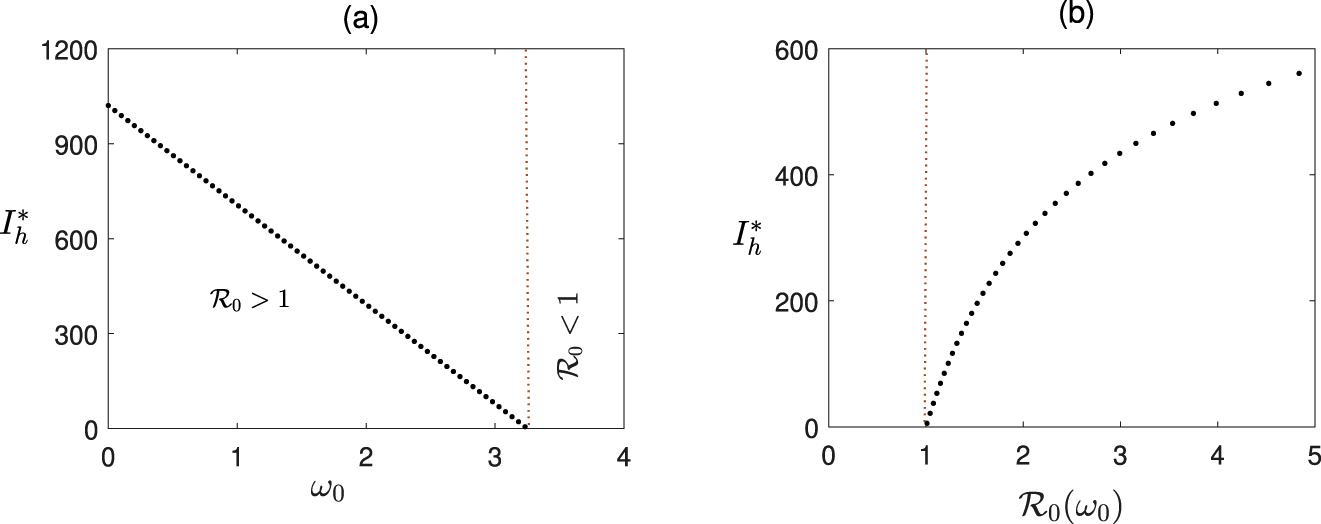
Transcritical bifurcation: Effect of ω 0 (global awareness) on the size of the epidemic and stability of disease-free equilibrium E ₀. Values of the parameters are taken from Table 1.

It can be noted that according to Theorem 3, the stability of the disease-free equilibrium does not depend on the time delay τ, rather on the basic reproduction number ℛ₀ only. So if we can keep the value of ℛ₀ below 1, the disease-free steady state would be stable for any τ > 0 . At ℛ₀ = 1, a transcritical bifurcation occurs, and the system becomes endemic. In Figure 2, the impact of local awareness ω on infected cases is shown. As ω increases infected humans decrease.

Figure 2:

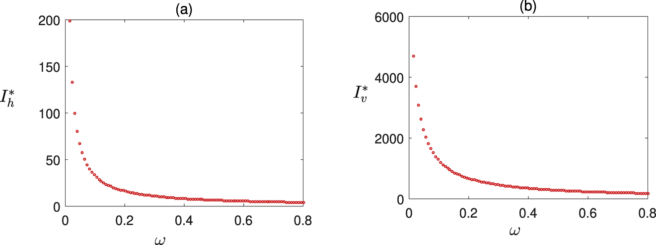
Effect of ω (local awareness) on the size of the epidemic. Values of the parameters are taken from Figure 1.

Figure 3 illustrates how stability of the endemic steady state depends on the disease transmission rates α 0 and β 0 . We observe that the product of transmission rate α 0 from vector to human and β 0 from human to vector has to exceed some threshold value for the endemic steady state to be feasible, and for smaller values of this product the endemic state is stable but then also loses its stability.

Figure 3:

Region of stability of equilibria in α 0 − β 0 parameter plane: (a) disease-free, (b) endemic equilibrium. Rest of the parameters are taken from Figure 1. Color code denotes the max [ R e   ξ ] at steady state. In white region of both the figures, endemic equilibrium E ^* is not feasible.

Figure 4 shows that the endemic equilibrium only exists for a limited range of disease transmission rates, and it is stable for higher rates and unstable for smaller α 0 . Increasing the local awareness rate ω leads to a destabilization of the endemic steady state, but surprisingly, increasing a global awareness rate ω 0 or a local awareness rate ω actually results in stabilizing an endemic steady state, whilst increasing these rates above certain values makes the endemic steady state unfeasible, in which case the disease-free steady state is stable.

Figure 4:

Region of stability of equilibria in ω 0 − β 0 and ω 0 − α 0 parameter plane: (a) disease-free, (b) endemic equilibrium. Rest of the parameters are taken from Figure 1. Color code denotes the max [ R e   ξ ] at E ^*. In white region of both the figures, endemic equilibrium E ^* is not feasible.

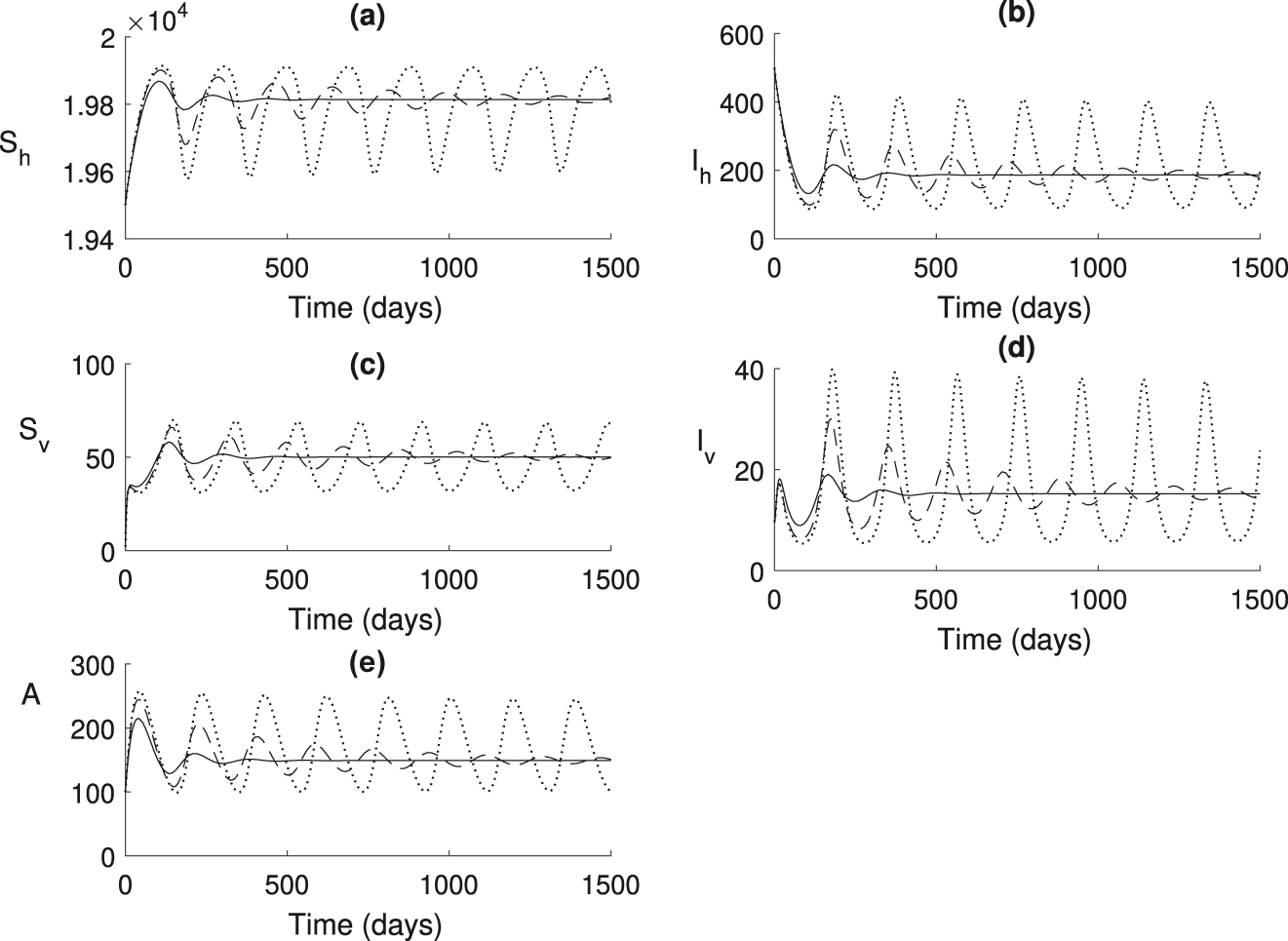
In Figure 5, choosing parameters in the range where ℛ₀ > 1 and increasing the time delays τ, resulting in the system approaching endemic steady state in an oscillatory manner, with the amplitude of oscillations increasing with the time delay. Once the time delay exceeds the critical value τ 0 , determined by Theorem 5, the endemic steady state becomes unstable via Hopf bifurcation, and the system exhibits stable periodic solutions. Figure 6 further illustrates the bifurcation diagram of endemic steady state E ^* taking τ as the bifurcation parameter. Minima and maxima of this solution suggests that the amplitude of oscillations itself increases with τ.

Figure 5:

Numerical solution of model (6) populations for different values of delay, τ. Parameters are taken from Table 1. Solid line is for τ = 0 , dashed line for τ = 12 and dotted line is for τ = 18 .

Figure 6:

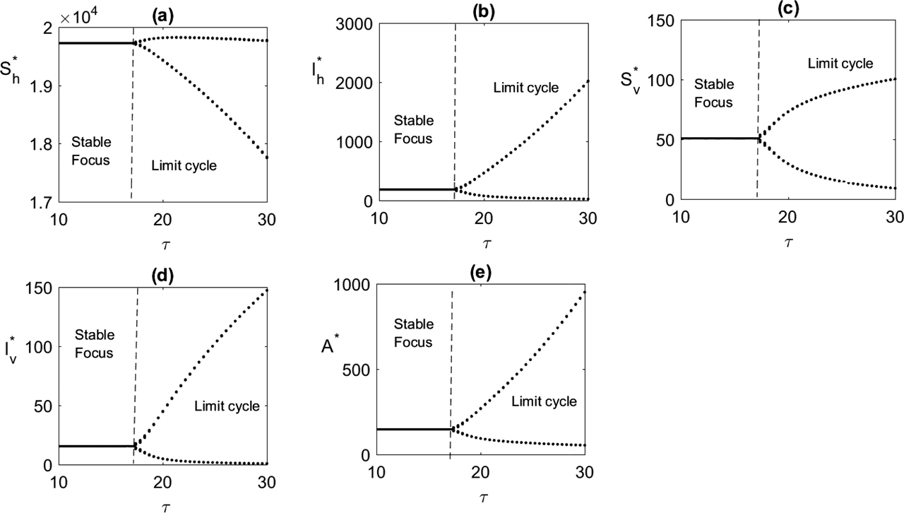
Bifurcation diagram is plotted taking τ as the main parameter. Parameters are taken from Table 1.

Figure 7 illustrates how the critical value τ 0 depends on different parameters. If disease transmission rate α 0 increases, Hopf bifurcation can be observed for lower value of τ. It also suggests that critical value τ 0 increases as the global awareness level ω 0 increases. Delay-induced oscillation can be reduced if both disease transmission rate is lowered and increasing the level of awareness.

Figure 7:

Region of stability of endemic equilibrium: (a) in τ − β 0 parameter plane taking parameters from Table 1, (b) in  τ − ω 0 parameter plane taking the parameters from Table 1 except α 0 = 0.00005 , β 0 = 0.00005 . Color code denotes the max [ R e   ξ ] at E ^*. In white region of both the figures, endemic equilibrium E ^* is not feasible.

Effect of global awareness ω 0 is plotted in Figure 8. The periodic oscillation disappears for higher rate of global awareness. Thus the awareness campaign through radio, TV etc. is very important for malaria disease control and also for mosquito population control.

Figure 8:

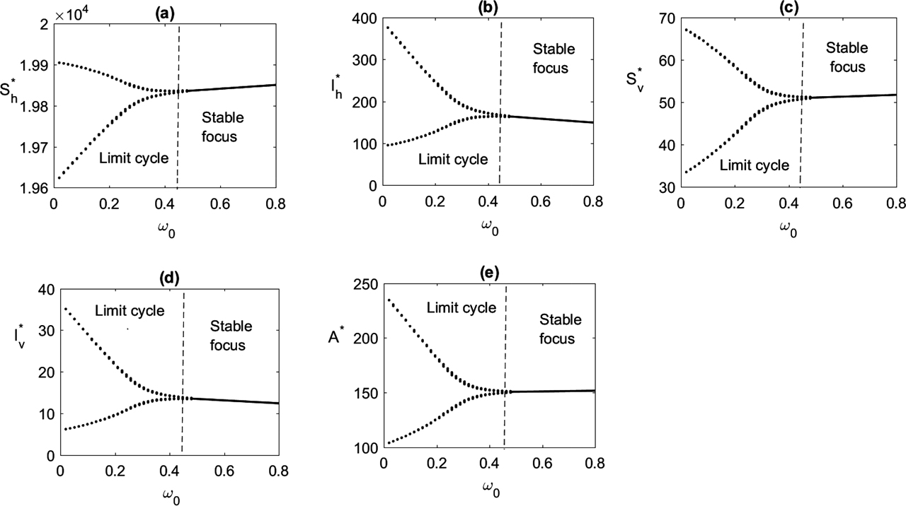
Bifurcation diagram is plotted taking ω 0 (global awareness) as the main parameter. Values of the parameters are taken from Table 1.

In Figure 9, we have shown the effect of insecticide on the delayed system. Periodic oscillation disappears and the endemic equilibrium becomes stable when γ 0 crosses the critical value γ 0 * = 0.5827 . This shows that insecticide spraying is sensitive for malaria disease control.

Figure 9:

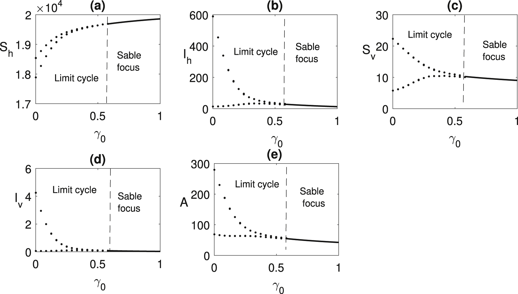
Bifurcation diagram is plotted taking γ 0 (rate of insecticide spraying) as the main parameter. Values of the parameters are taken from Table 1.

7 Discussion

Successful control of any vector-borne disease follows several factors including, but not limited to well-planned eradication strategies, targeted control measures to prevent spread of disease and also increase of awareness among the general mass. While inception of eradication programs require commitment from the higher authorities—namely policy makers—similar burden also falls on the common people to gather knowledge and increase awareness among themselves. This awareness is generated via effective expansion and improvement of case management, and through successive spread of the information [47].

In this article, the impact of awareness-based intervention for malaria control has been studied. For this, a mathematical model is derived considering SIS type sub-model for humans and SI sub-model for mosquitoes and the level of awareness as a separate population. We have assumed the disease transmission rates, vector to human and human to vector as decreasing function of the level of awareness, A (t). Model analysis shows two feasible equilibria namely the disease-free and endemic equilibrium. Disease-free equilibrium is stable until the value of the basic reproduction number, ℛ₀ < 1, but as the value of ℛ₀ exceeds 1, it becomes unstable, and numerically we see that endemic equilibrium exists for ℛ₀ > 1, which is a standard result in epidemiology. There exists a minimum awareness level ω 0 min such that we can rely on awareness for malaria eradication (Remark 1). The endemic equilibrium, whenever exists, is locally asymptotically stable when the delay τ is below the threshold value τ 0 . It becomes unstable through Hopf bifurcation if the delay parameter crosses the critical value τ 0 . We have seen that the critical value of τ depends on other parameters [10] namely global awareness rate ω 0 and awareness activity rate γ 0 (Figures 6–8).

The model analysis suggests that level of awareness among people has enough potential to mobilize higher fraction of the population. Increasing the awareness through radio, TV etc., the abundance of mosquitoes will be reduced in the environment and hence disease can be controlled. Moreover, it is found that media coverage has a substantial effect on the basic reproduction number, ℛ₀. Also, by continuous efforts and effectual media coverage with tolerable delay disease can be eradicated.

While spread of successful control strategies adds to the awareness about a disease, it is not uncommon that this knowledge is diluted over certain periods of time. In these cases, debates may arise that shift the focus from the actual course of action that needs to be selected. These shortcomings should be included in the mathematical models to find their relevance.

References

[1] World Health Organization, World Malaria Report, 2015, Geneva, Switzerland, WHO, 2015.Search in Google Scholar
[2] World Health Organization, World Malaria Report 2017, Geneva, WHO, 2017.Search in Google Scholar
[3] World Health Organization, World Malaria Report 2019, Geneva, Switzerland, WHO, 2019.Search in Google Scholar
[4] L. Cai, X. -Z. Li, N. Tuncer, M. Martcheva, and A. A. Lashari, “Optimal control of a malaria model with asymptomatic class and superinfection,” Math. Biosci., vol. 288, pp. 94–108, 2017. https://doi.org/10.1016/j.mbs.2017.03.003.Search in Google Scholar PubMed
[5] G. A. Ngwa, “On the population dynamics of the malaria vector,” Bull. Math. Biol., vol. 68, pp. 2161–2189, 2006. https://doi.org/10.1007/s11538-006-9104-x.Search in Google Scholar PubMed
[6] C. N. Ngonghala, S. Y. Del Valle, R. Zhao, and J. Mohammed-Awel, “Quantifying the impact of decay in bed-net efficacy on malaria transmission,” J. Theor. Biol., vol. 363, pp. 247–261, 2014. https://doi.org/10.1016/j.jtbi.2014.08.018.Search in Google Scholar PubMed PubMed Central
[7] S. Kim, M. A. Masud, and G. Cho, “Analysis of a vector-bias effect in the spread of malaria between two different incidence areas,” J. Theor. Biol., vol. 419, pp. 66–76, 2017. https://doi.org/10.1016/j.jtbi.2017.02.005.Search in Google Scholar PubMed
[8] A. K. Misra, A. Sharma, and J. Li, “A mathematical model for control of vector borne diseases through media campaigns,” Discrete Continuous Dyn. Syst. Ser. B (DCDS-B), vol. 18, no. 7, 2013. https://doi.org/10.3934/dcdsb.2013.18.1909.Search in Google Scholar
[9] P. Rani, D. Jain, and V. P. Saxena, “Stability analysis of HIV/AIDS transmission with treatment and role of female sex workers,” Int. J. Nonlinear Sci. Numer. Stimul., vol. 18, no. 6, pp. 457–467, 2017. https://doi.org/10.1515/ijnsns-2015-0147.Search in Google Scholar
[10] G. O. Agaba, Y. N. Kyrychko, and K. B. Blyuss, “Dynamics of vaccination in a time-delayed epidemic model with awareness,” Math. Biosci., vol. 294, pp. 92–99, 2017. https://doi.org/10.1016/j.mbs.2017.09.007.Search in Google Scholar PubMed
[11] A. K. Misra, R. K. Rai, and Y. Takeuchi, “Modeling the control of infectious diseases: effects of TV and social media advertisements,” Math. Biosci. Eng., vol. 15, no. 6, pp. 1315–1343, 2018. https://doi.org/10.3934/mbe.2018061.Search in Google Scholar PubMed
[12] P. Gupta, A. R. Anvikar, N. Valecha, and Y. K. Gupta, “Pharmacovigilance practices for better healthcare delivery: knowledge and attitude study in the national malaria control programme of India,” Malar. Res. Treat., vol. 2014, 2014, Art no. 837427. https://doi.org/10.1155/2014/837427.Search in Google Scholar PubMed PubMed Central
[13] M. K. Chourasia, K. Raghavendra, R. M. Bhatt, D. K. Swain, G. D. P. Dutta, and I. Kleinschmidt, “Involvement of Mitanins (female health volunteers) in active malaria surveillance, determinants and challenges in tribal populated malaria endemic villages of Chhattisgarh, India,” BMC Publ. Health, vol. 18, no. 1, p. 9, 2018. https://doi.org/10.1186/s12889-017-4565-4.Search in Google Scholar PubMed PubMed Central
[14] F. Kasteng, J. Murray, S. Cousens, et al.., “Cost-effectiveness and economies of scale of a mass radio campaign to promote household life-saving practices in Burkina Faso,” BMJ Glob. Health, vol. 3, no. 4, p. e000809, 2018. https://doi.org/10.1136/bmjgh-2018-000809.Search in Google Scholar PubMed PubMed Central
[15] E. B. Fokam, G. F. Kindzeka, L. Ngimuh, K. T. J. Dzi, and S. Wanji, “Determination of the predictive factors of long-lasting insecticide-treated net ownership and utilisation in the Bamenda health district of Cameroon,” BMC Publ. Health, vol. 17, no. 1, p. 263, 2017. https://doi.org/10.1186/s12889-017-4155-5.Search in Google Scholar PubMed PubMed Central
[16] L. Alphey, C. B. Beard, P. Billingsley, et al.., “Malaria control with genetically manipulated insect vectors,” Science, vol. 298, no. 5591, pp. 119–121, 2002. https://doi.org/10.1126/science.1078278.Search in Google Scholar PubMed
[17] S. K. Ghosh and A. P. Dash, “Larvivorous fish against malaria vectors: a new outlook,” Trans. R. Soc. Trop. Med. Hyg., vol. 101, no. 11, pp. 1063–1064, 2007. https://doi.org/10.1016/j.trstmh.2007.07.008.Search in Google Scholar PubMed
[18] Y. Lou and X. Q. Zhao, “Modelling malaria control by introduction of larvivorous fish,” Bull. Math. Biol., vol. 73, no. 10, pp. 2384–2407, 2011. https://doi.org/10.1007/s11538-011-9628-6.Search in Google Scholar PubMed
[19] D. Kumar, J. Singh, M. Al Qurashi, and D. Baleanu, “A new fractional SIRS-SI malaria disease model with application of vaccines, antimalarial drugs, and spraying,” Adv. Differ. Equ., vol. 2019, no. 1, p. 278, 2019. https://doi.org/10.1186/s13662-019-2199-9.Search in Google Scholar
[20] J. C. Kamgang and C. P. Thron, “Analysis of malaria control measures’ effectiveness using multistage vector model,” Bull. Math. Biol., vol. 81, no. 11, pp. 4366–4411, 2019. https://doi.org/10.1007/s11538-019-00637-6.Search in Google Scholar PubMed
[21] M. Runge, F. Molteni, R. Mandike, et al.., “Applied mathematical modelling to inform national malaria policies, strategies and operations in Tanzania,” Malar. J., vol. 19, no. 1, pp. 1–10, 2020. https://doi.org/10.1186/s12936-020-03173-0.Search in Google Scholar PubMed PubMed Central
[22] F. Chamchod and N. F. Britton, “Analysis of a vector-bias model on malaria transmission,” Bull. Math. Biol., vol. 73, pp. 639–657, 2011. https://doi.org/10.1007/s11538-010-9545-0.Search in Google Scholar PubMed
[23] C. J. Silva and D. F. M. Torres, “An optimal control approach to malaria prevention via insecticide-treated nets,” Conf. Papers Math., vol. 2013, 2013, Art no. 658468. https://doi.org/10.1155/2013/658468.Search in Google Scholar
[24] F. B. Agusto, S. Y. Del Valle, K. W. Blayneh, et al.., “The use of bed net use on malaria prevalence,” J.Theor. Biol., vol. 320, pp. 58–65, 2013. https://doi.org/10.1016/j.jtbi.2012.12.007.Search in Google Scholar
[25] N. Chitnis, A. Schapira, T. Smith, and R. Steketee, “Comparing the effectiveness of malaria vector-control interventions through a mathematical model,” Am. J. Trop. Med. Hyg., vol. 83, no. 2, pp. 230–240, 2010. https://doi.org/10.4269/ajtmh.2010.09-0179.Search in Google Scholar
[26] M. T. White, R. Verity, T. S. Churcher, and A. C. Ghani, “Vaccine approaches to malaria control and elimination: insights from mathematical models,” Vaccine, vol. 33, no. 52, pp. 7544–7550, 2015. https://doi.org/10.1016/j.vaccine.2015.09.099.Search in Google Scholar
[27] M. Ghosh, S. Olaniyi, and O. Obabiyi, “Mathematical analysis of reinfection and relapse in malaria dynamics,” Appl. Math. Comput., vol. 373, p. 125044, 2020. https://doi.org/10.1016/j.amc.2020.125044.Search in Google Scholar
[28] J. Sequeira, J. Louçã, A. M. Mendes, and P. G. Lind, “Transition from endemic behavior to eradication of malaria due to combined drug therapies: an agent-model approach,” J. Theor. Biol., vol. 484, p. 110030, 2020. https://doi.org/10.1016/j.jtbi.2019.110030.Search in Google Scholar
[29] X. Wang and X. Zou, “Modeling the potential role of engineered symbiotic bacteria in malaria control,” Bull. Math. Biol., vol. 81, no. 7, pp. 2569–2595, 2019. https://doi.org/10.1007/s11538-019-00619-8.Search in Google Scholar
[30] H. Ishikawa, A. Kaneko, and A. Ishii, “Computer simulation of a malaria control trial in Vanuatu using a mathematical model with variable vectorial capacity,” Jpn. J. Trop. Med. Hyg., vol. 24, no. 1, pp. 11–19, 1996. https://doi.org/10.2149/tmh1973.24.11.Search in Google Scholar
[31] H. Ishikawa, A. Ishii, N. Nagai, et al.., “A mathematical model for the transmission of Plasmodium vivax malaria,” Parasitol. Int., vol. 52, no. 1, pp. 81–93, 2003. https://doi.org/10.1016/s1383-5769(02)00084-3.Search in Google Scholar
[32] S. Flessa, “Decision support for malaria control programmes–a system dynamics model,” Health Care Manag. Sci., vol. 2, no. 3, pp. 181–191, 1999. https://doi.org/10.1023/a:1019044013467.10.1023/A:1019044013467Search in Google Scholar
[33] S. Bhatt, D. J. Weiss, E. Cameron, et al.., “The effect of malaria control on Plasmodium falciparum in Africa between 2000 and 2015,” Nature, vol. 526, no. 7572, pp. 207–211, 2015. https://doi.org/10.1038/nature15535.Search in Google Scholar PubMed PubMed Central
[34] L. J. Zühlke and M. E. Engel, “The importance of awareness and education in prevention and control of RHD,” Glob. Heart, vol. 8, no. 3, pp. 235–239, 2013. https://doi.org/10.1016/j.gheart.2013.08.009.Search in Google Scholar PubMed
[35] S. Ruan, D. Xiao, and J. C. Beier, “On the delayed Ross–MacDonald model for malaria transmission,” Bull. Math. Biol., vol. 70, no. 4, pp. 1098–1114, 2008. https://doi.org/10.1007/s11538-007-9292-z.Search in Google Scholar PubMed PubMed Central
[36] E. Agyingi, T. Wiandt, and M. Ngwa, “Stability and Hopf bifurcation of a two species malaria model with time delays,” Lett. Biomath., vol. 4, no. 1, pp. 59–76, 2017. https://doi.org/10.1080/23737867.2017.1296383.Search in Google Scholar
[37] H. Wan and J. Cui, “A malaria model with two delays,” Discrete Dynam Nat. Soc., vol. 2013, 2013, Art no. 601265. https://doi.org/10.1155/2013/601265.Search in Google Scholar
[38] G. A. Ngwa, C. N. Ngonghala, and N. B. S. Wilson, “A model for endemic malaria with delay and variable populations,” J. Cameroon Acad. Sci, vol. 1, no. 3, pp. 168–186, 2001.Search in Google Scholar
[39] H. Xiang, M. X. Zou, and H. F. Huo, “Modeling the effects of health education and early therapy on tuberculosis transmission dynamics,” Int. J. Nonlinear Sci. Numer. Stimul., vol. 20, nos 3–4, pp. 243–255, 2019. https://doi.org/10.1515/ijnsns-2016-0084.Search in Google Scholar
[40] F. Al Basir, S. Ray, and E. Venturino, “Role of media coverage and delay in controlling infectious diseases: a mathematical model,” Appl. Math. Comput., vol. 337, pp. 372–385, 2018. https://doi.org/10.1016/j.amc.2018.05.042.Search in Google Scholar
[41] F. Al Basir, “Dynamics of infectious diseases with media coverage and two time delay,” Math. Models Comput. Simul., vol. 10, no. 6, pp. 770–783, 2018. https://doi.org/10.1134/s2070048219010071.Search in Google Scholar
[42] D. Greenhalgh, S. Rana, S. Samanta, T. Sardar, S. Bhattacharya, and J. Chattopadhyay, “Awareness programs control infectious disease–multiple delay induced mathematical model,” Appl. Math. Comput., vol. 251, pp. 539–563, 2015. https://doi.org/10.1016/j.amc.2014.11.091.Search in Google Scholar
[43] F. Al Basir, K. B. Blyuss, and S. Ray, “Modelling the effects of awareness-based interventions to control the mosaic disease of Jatropha curcas,” Ecol. Complex., vol. 36, pp. 92–100, 2018. https://doi.org/10.1016/j.ecocom.2018.07.004.Search in Google Scholar
[44] J. Hale, Theory of Functional Differential Equations, NY, Heidelberg, Berlin, Springer-Verlag, 1977.10.1007/978-1-4612-9892-2Search in Google Scholar
[45] J. M. HefferNan, R. J. Smith, and L. M. Wahl, “Perspectives on the basic reproductive ratio,” J. R. Soc. Interface, vol. 2, no. 4, pp. 281–293, 2005. https://doi.org/10.1098/rsif.2005.0042.Search in Google Scholar PubMed PubMed Central
[46] T. Zhang, H. Jiang, and Z. Teng, “On the distribution of the roots of a fifth degree exponential polynomial with application to a delayed neural network model,” Neurocomputing, vol. 72, pp. 1098–1104, 2009. https://doi.org/10.1016/j.neucom.2008.03.003.Search in Google Scholar
[47] L. M. Barat, “Four malaria success stories: how malaria burden was successfully reduced in Brazil, Eritrea, India, and Vietnam,” Am. J. Trop. Med. Hyg., vol. 74, no. 1, pp. 12–16, 2006. https://doi.org/10.4269/ajtmh.2006.74.12.Search in Google Scholar
© 2020 Fahad Al Basir et al., published by De Gruyter, Berlin/Boston
This work is licensed under the Creative Commons Attribution 4.0 International License.
Articles in the same Issue
- Frontmatter
- Original Research Articles
- Research on prediction model of thermal and moisture comfort of underwear based on principal component analysis and Genetic Algorithm–Back Propagation neural network
- Design of the state feedback-based feed-forward controller asymptotically stabilizing the double-pendulum-type overhead cranes with time-varying hoisting rope length
- Blowup and global existence of mild solutions for fractional extended Fisher–Kolmogorov equations
- Lipschitz stability of nonlinear ordinary differential equations with non-instantaneous impulses in ordered Banach spaces