
Harris hawks optimization algorithm for load frequency control of isolated multi-source power generating systems
-
Yannis L. Karnavas

 and
Evaggelia Nivolianiti
and
Evaggelia Nivolianiti

Abstract
This paper presents a recent bio-inspired optimization algorithm for the critical topic of load frequency control (LFC) in an isolated multi-source power generating system. A specific model that emerges from the scientific literature and consists of reheated thermal, hydro and gas-turbine power sources is examined. The main goal is to tune the controller of each generating source i.e. find their optimal gains through bio-inspired optimization algorithms. Namely, the algorithms applied are the Whale Optimization Algorithm (WOA), Grey Wolf Optimizer (GWO), Particle Swarm Optimization (PSO), and the newly proposed Harris Hawks Optimization (HHO). It was observed that all optimization algorithms succeeded in obtaining controllers’ gain values which ensure stable system operation. Also, the simulation results indicated the superiority of the proposed HHO algorithm over the other algorithms for all the considered scenarios. In this article, for the first time to the authors’ knowledge extend an attempt has been made to optimize an isolated multi-source system using the bio-inspired HHO algorithm. The present study considered the LFC problem with a variety of different scenarios, taking into account both sub-cases of nonlinearities (e.g., generation rate constraint, boiler dynamics, etc.) and their combinations, as well as combinations of different controllers and load disturbances, which are not found in the literature. Last but not least, the robustness of the selected controller was further evaluated. The obtained results clearly demonstrated that the controller’s gains established in normal conditions do not require retuning when critical system parameters undergo a significant variation.
1 Introduction
Load frequency control (LFC) is one of the primary procedures of the automatic generation control (AGC) scheme in a power generating system. It is a significant control problem relevant to electric power system operation, which has been a research subject for the last decades and still remains an important research topic. It is well known that the reliability and stability of an electrical power system depend mainly on its frequency deviation from the pre-defined (or nominal) value [1]. Many undesirable effects could happen in the opposite case, e.g., from partial load shedding up to total “black-out” situations. Generally, a frequency deviation in power systems is caused by a power imbalance between demand and generation [2]. In cases of deviations, LFC aims to return the frequency and, in the case of interconnected systems, the power exchange to the predetermined levels. In recent decades, researchers have been trying to find new approaches for LFC to maintain the frequency as well as the AC voltages at specific values against if possible a large range of disturbances (e.g., Refs. [3, 4]).
The power generating system examined and discussed in this paper has been studied in the past with different kinds of controllers, different types of algorithms and different corresponding objective functions. The authors of Refs. [5, 6], adopted the genetic algorithm (GA) to adjust the controllers of the system, and also made a comparison between a common PI controller for all three sources and an individual PI controller for each separate source. The criteria used in both studies were the integral-in-time absolute error (ITAE) and the integral squared error (ISE), while in the latter study [6], the case of adopting a generation rate constraint (GRC) to the system was also considered, which actually increases the problem’s non-linearity. In Ref. [7], the same system was examined but with the water cycle (WCA) algorithm, by employing a PI controller and utilizing the ITAE criterion. In Ref. [8], the grey wolf optimization (GWO) algorithm was employed for setting PID controllers’ gains. Continuing, in Ref. [9], three different algorithms were utilized and compared, namely the moth-flame optimizer (MFO), the differential evolution (DE) and the teaching learning-based optimization (TLBO). Moreover, in Ref. [10], three different kinds of controllers were applied and compared, called PID Ziegler-Nichols Open Loop (PID-ZN-OL), PID Chien-Hrones-Reswick (PID C-H-R) and fuzzy PID. Both [11, 12], considered the power system with the difference that the former used stochastic fractal search (SFS) and local unimodal sampling (LUS) while the latter employed particle swarm optimization (PSO) to tune PID controllers.
On the other hand, there is quite a bit of literature in which the particular system of an islanded power generating system is extended to interconnected areas. References [13], [14], [15], considered both an islanded and an interconnected system. In Ref. [13] many different controllers and criteria were compared, i.e. PID, PI and I controllers were presented and DE was employed considering ITAE, ISE, integral-in-time square error (ITSE) and integral absolute error (IAE) performance indices, while [14] utilized a PID cascade controller through the dragonfly algorithm (DA). In Ref. [15] the performance of imperialist competitive algorithm (ICA), differential evolution, teacher learning based optimization and hybrid stochastic fractal search (hSFS) was compared. Also, in Refs. [16, 17], both islanded and two-area power systems were examined in combination with a lumped PEV (plug in electric vehicle). In the first, a modified grey wolf optimization (mGWO) for setting PI, PID, PIPD controllers’ gains was introduced while in the second a stochastic fractal search was proposed.
As can be seen from the above-mentioned references, the use of metaheuristic methods has become more popular than traditional methods for solving optimization problems. That’s because they are easy to use and provide reliable results. In recent years, swarm-based bio-inspired algorithms have proven to be highly successful in solving various optimization problems. This study implemented a newly developed swarm-based optimization approach known as the Harris Hawks Optimization (HHO) algorithm. HHO is a gradient-free optimization algorithm with several active and time-varying phases of exploration and exploitation of the search space [18]. According to [19], this algorithm can lead to improved results compared to other optimization algorithms such as MFO, whale optimization algorithm (WOA), cuckoo search (CS), PSO, DE and GWO. Some studies have reported the application of the HHO algorithm for LFC in multi-area power systems. For example, in Ref. [20] a thermal-solar interconnected system with two types of controllers (PID and 1-FOID) were studied. In Ref. [21] three different kinds of controllers such as the TID, IDDF and cascaded PIDN-TIDF for a three-area power system were examined. Finally, in Refs. [18, 22, 23] a comparison between HHO and other algorithms such as the GA, the bacterial foraging optimization (BFO), PSO and the TLBO was performed and it was shown that HHO gave superior results than the others.
However, HHO has not been applied to LFC problems in isolated multi-source systems until recently. In this study, the HHO was used in order to optimally tune three different controller topologies, i.e. a PI, a PID and a FOPID for the LFC problem of a single-area multi-source system. Furthermore, the effectiveness of the suggested approach was assessed by comparing its performance with other commonly used bio-inspired optimization methods such as WOA, GWO and PSO, providing a comprehensive analysis of the controller’s performance. The key contributions of this work can be summarized as follows:
An analysis of the dynamic behavior of a realistic (single-area multi-source) power generation system made up of a reheat thermal unit, a hydro unit, and a gas unit, was performed. Non-linearities such as GRC, governor deadband (GDB) and boiler dynamics (BD) were incorporated into the model.
The performance of various metaheuristic optimization algorithms, including WOA, GWO, PSO and the newly proposed HHO, was evaluated. This assessment aimed to provide valuable insights into determining the most suitable algorithm for the specific application being studied.
The performance of different controllers, specifically PI, PID and FOPID, was assessed. The analysis involved studying the system dynamics while considering a variety of different scenarios, taking into account both sub-cases of nonlinearities (e.g., generation rate constraint, boiler dynamics, etc.) and their combinations, as well as combinations of different load disturbances, which are not found in the literature. This comprehensive analysis aimed to provide a thorough understanding of the system dynamics and demonstrate the effectiveness of the controllers in regulating the frequency of the system.
The sensitivity of the proposed HHO-tuned controllers to variations in system parameters was examined. By analyzing the sensitivity, the research provides information on the controller’s resilience and identifies how certain parameters influence its effectiveness.
In the above context, the paper is structured as follows: Section 2 analyzes the power generation system under study, along with the formulation of the utilized controllers and performance criteria. A brief description of the employed HHO algorithm is then given in Section 3. The examined scenarios, along with the corresponding results, are presented and discussed in Section 4. Further analysis of the designed controller’s robustness is elaborated in Section 5. The work is finally concluded in Section 6 while the pertinent system data are given for clarity in the Appendix.
2 Multi-source power generating system under study
2.1 System overview
In this work, LFC is examined in an isolated multi-source power system. The system under consideration consists of a reheated thermal-turbine power source, a hydro-turbine power source and a gas-turbine power source [5]. Figure 1 depicts the equivalent small signal perturbation block diagram. Under normal conditions, there is no inequality between production and demand and the following relationship holds [23]:
where the power of the steam generation source P Gs = K s P G , power of the hydro generation source P Gh = K h P G and power of the gas generation source P Gg = K g P G . The K s , K h and K g are the sources’ participation factors (spf), which may be used for systems with more than one type of source per control area, like the one examined here. In some studies, source participation factors divide the power of each area’s loads equally, so that all units serve the corresponding portion of the demand, but this is not true in real systems whereas the demand is divided according to the availability of the generators comprising the source [5]. However, in any case, the following constraint applies [23]:
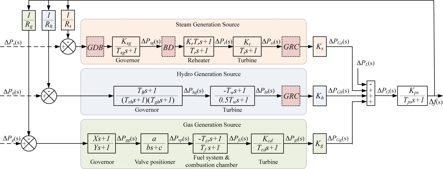
Isolated multi-source power system under study (uncontrolled).
In this particular system, the total power is 1750 MW, of which the steam, hydro and gas sources contribute 1000 MW, 500 MW and 250 MW respectively (ratio of 4:2:1). In this loading condition, the participation coefficients are derived and given in the Appendix along with all the other system parameters. The power system subsystem in Figure 1 can be modeled under the assumption that the power of the turbines is balanced by the power of the synchronous generators. The demanded load power is subject to continuous variations ΔP L (s), which must be covered by the generator’s power. The difference between generated power and demand creates a variation in the frequency Δf(s) of the system. The equilibrium equation is then given by the following relationship:
This equation can be written as [23]:
where K ps is the power system gain constant (in Hz/pu MW) and T ps is the power system time constant which can be obtained by [5]:
where H is the system inertia constant, D is the damping factor and f 0 is the system rated frequency.
2.1.1 Steam generation source
A steam power plant consists of subsystems which will be analyzed next. The speed governor valve controls the speed of the turbine. The turbine controls the rotational speed of the synchronous generator and hence its output power. The speed of the generator controls the position of the speed governor valve, with feedback. The process is repeated until the electrical power produced equals the system demand. As shown in Figure 1, the speed governor accepts the difference of two inputs. ΔP s (s) is the reference load signal and Δf(s)/R s is the frequency deviation signal. Thus, the output of the speed governor ΔP sg is a function of the difference between these two signals and is a corrective action. As long as the generated power is equal to the demand, the steam flow is constant. The role of the governor is to restore the imbalance between generated and demanded power. For example, if the load is momentarily reduced, the electric torque opposing the engine shaft will weaken. This results in an increase in the speed of the motor. The speed governor must then close the steam inlet valve to reduce the steam flow and balance the system. The transfer function of the speed governor is:
where T sg is the steam turbine speed governor time constant and K sg is the coefficient of the steam turbine speed governor. Thermal power plants often use a reheater in order to improve their efficiency. The subsystem of the reheater takes as input the output of the speed governor subsystem ΔP sg (s). ΔP r (s) is the output signal of the reheater and its transfer function is:
where T r is the reheater time constant and K r is the coefficient of the reheater steam turbine. The reheater subsystem’s output is fed into the turbine-generator subsystem. The output signal of the steam turbine is ΔP st (s) and its transfer function is:
where T t is the steam turbine time constant and K t is the coefficient of the steam turbine.
2.1.2 Hydro generation source
Hydro power plants are modeled according to the same basic principles. The complete model is analyzed next. In this case, the speed regulation is achieved by using a governor (mechanical-hydraulic) which controls the water supply to the turbine. If there is a discrepancy between the power produced and the power demanded, a differential control signal is returned to the regulator. For example, if the demand increases then the water flow should also increase through the position of the water intake valve. As the water flow increases, the mechanical torque at the turbine outlet increases. With respect to Figure 1, the first block diagram, modeling the operation of a mechanical-hydraulic speed governor, consists of two blocks in series. The first block is the motor pilot stage that drives the second block, which models the servo that controls the water intake valve. As long as the generated power is equal to the demand, the water flow is constant. When there is a disturbance in the system, the speed controller reacts to restore balance. Thus, the transfer function of the speed governor is as follows:
The mechanical-hydraulic governor accepts the difference between two inputs. ΔP h (s) is the reference load signal and Δf(s)/R h is the frequency deviation signal. As a result, the output of the governor ΔP hg (s) is a function of the difference between these two signals. T R is the hydro turbine speed governor reset time, T rh is the transient droop time constant and T gh is the main servo time constant. Regarding the hydro turbine subsystem, this is modeled by a block that converts the mechanical input power into electrical power. The transfer function between input ΔP hg (s) and output ΔP ht (s) is as follows:
where T w is penstock water time constant.
2.1.3 Gas generation source
The last power generation source shown in Figure 1, is that of a complete gas turbine power plant. Each subsystem will be analyzed separately below. As it is well known, gas turbine plants consist of a turbine, which turns the generator, a combustion chamber and a compressor, also driven by the turbine. Similar to the speed governor subsystem in a steam power plant, the subsystem of a gas turbine power plant models the balance control between generated and demanded power. As shown in the figure, ΔP g (s) is the reference load signal and Δf(s)/R g is the frequency deviation signal. Thus, the output of the speed controller ΔP gg (s) is a function of the difference between the aforementioned two signals and it actually implements a corrective action described by the following transfer function:
where X, Y are the gas turbine speed governor lead time constant and lag time constant, respectively. The speed governor sub-system drives a secondary stage called the valve positioner sub-system. This subsystem controls the position of the fuel inlet valve to ensure a balance between the power produced and the power demanded. The transfer function between input ΔP gg (s) and output ΔP vp (s) is:
where a, c are the gain constants of the valve positioner and b is the time constant of the valve positioner. In the fuel and combustion chamber subsystem, the chemical reactions of combustion take place, which produce the thermal energy that drives the gas turbine. This stage gives as output ΔP fc (s) signal and has the following transfer function:
where T cr is the combustion chamber reaction time delay and T f is the fuel time constant. Finally, the turbine dynamics subsystem models the behavior of the turbine and the synchronous three-phase generator to which it is connected. The transfer function of the subsystem is:
The turbine dynamics accepts as input the output of the fuel subsystem ΔP fc (s) and gives as output ΔP gt (s). The K cd and T cd represent the compressor discharge volume coefficient and time constant, respectively.
2.2 System inherent non-linearities
In real power plants, restrictions apply (in the form of non-linearities) known as generation rate limits which exist on the rate of change in power generation and also in the governor’s action. The first is called generation rate constraint (GRC), while the latter is called governor’s dead band (GDB). In literature, these two restrictions are usually met in steam and hydro power sources. Also, in a steam source, boiler dynamics (BD) can be considered in LFC studies, which also impose increased non-linearity on the system. The block diagrams of these constraints are shown in Figure 2 and are explained next.

With respect to Figure 1: (a) boiler dynamics block diagram (BD), (b) governor dead-band dynamics (GDB), and (c) generation rate constraint block diagram (GRC).
2.2.1 Boiler dynamics
The BD represents a device that is intended to produce steam under pressure. Practically, such a boiler responds very quickly during sudden load demand in thermal power plants. A simplified non-linear model of a boiler’s dynamic is shown in Figure 2(a). The time constant of the combustion system is T fb , while T D denotes the time delay before a change command is executed. The boiler is shown as an integrator with an output of normalized pressure and a time constant C B proportional to its capacity [24].
2.2.2 Governor dead band
GDB is defined as the zone of extended speed change within which there is no change in valve (fuel rack) position. The combined transfer function of the GDB and the steam governor is Ref. [15]:
where N 1 and N 2 are set as 0.8 and −0.2/π, respectively The block diagram is shown in Figure 2(b).
2.2.3 Generation rate constraint
Figure 2(c) depicts the block diagram of the GRC, which is responsible for limiting the generation rate and is related to the speed at which the generating unit varies its output power. There are normally two limits that can be used to control how quickly the generation of electricity from different sources changes (high and low). In the literature, these limits for steam power plants range from 3 to 10 %/min. A value of 10 %/min was chosen in our study. Moreover, the corresponding limits for hydro power source are set to 270 %/min and 360 %/min for the upper and lower limits respectively [17].
2.3 Control strategy and optimization function
The main step in testing the controller design with an optimization algorithm is to choose appropriate objective functions. The integral absolute error (IAE), integral-squared error (ISE), integral-time-squared error (ITSE), and integral time absolute error (ITAE) are examples of integral-based objective functions. In contrast to the ITAE, the ISE, IAE and ITSE criteria require longer settling times and cannot always perform within a desirable stability margin [25, 26]. The literature has shown that the ITAE is more effective than other performance criteria. The ITAE is used as the optimization objective function for the controller gains in this study, and it is given by:
where T sim is the time range of the simulation and Δf is the frequency deviation of the system.
As mentioned in the introduction Section, there are many configurations of controller types that may be used in LFC studies. In the current study, the system has been modeled using a PI, PID and FOPID controller for each plant in MATLAB/Simulink environment.
2.3.1 PI controller
The PI controller is described by the well-known transfer function:
where K p is the proportional gain and K i is the integral gain. In this context, the optimization of the fitness function of the problem can be given as:
under the constraints:
where,
2.3.2 PID controller
The transfer function for the PID controller is provided by:
where, K p , K i , K d are the proportional, integral and derivative gains, respectively. The optimization of the fitness function in this case is given as:
under the constraints:
The minimum and maximum controller gain values are chosen to be −50 and 50, respectively.
2.3.3 FOPID controller
A fractional-order PID (FOPID) controller is a type of control that has several advantages. One of the main advantages is improved robustness and flexibility, meaning that FOPID controllers are more resistant to parameter variations and external disturbances, allowing for stable control of the system even when there are changes in the system dynamics. Furthermore, FOPID controllers can achieve a faster response time and better steady-state performance than traditional PID controllers. The mathematical expression can be given as:
where μ is a differential order and λ is an integral order to provide the PID controller’s settings with a larger tuning range [27]. The optimization of the fitness function in this case is given by:
under the constraints:
The minimum and maximum gain values of controller gains (K p , K i , K d ) are chosen to be −50 and 50, respectively and the value range of μ and λ is [0, 5].
3 Harris hawk optimization algorithm
Examining the Harris hawks nature reveals that while they can follow and identify their prey, the prey may not always be readily visible. The prey may come after several hours, so the hawks wait, watch, and monitor the area in order to find it. Figure 3 shows all the HHO algorithm phases and their brief mathematical background is given next [28].
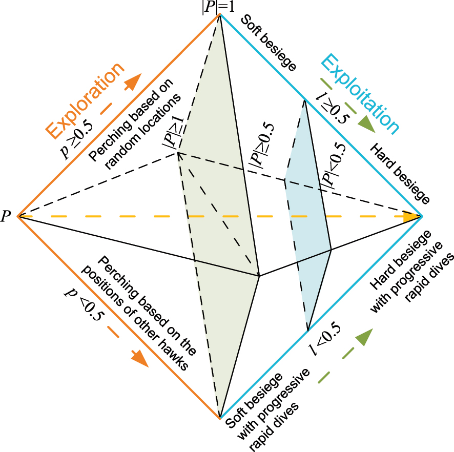
Harris hawk optimization algorithm strategy.
3.1 Exploration phase
The candidate solutions in this algorithm are hawks, and at each phase the ideal candidate solution is regarded as the desired prey. The algorithm predicts that hawks will randomly roost in some places and wait until they spot a prey using two different tactics. Assuming equal probability p between (0, 1) for each tactic, the hawks either roost according to where the other group members are located (so that they are close to them when they attack) and the position of the hare, a first strategy modeled for p < 0.5, or they roost randomly in tall trees (random locations within the group area), a second strategy modeled for p ≥ 0.5.
where v 1, v 2, v 3, and v 4 are random integers between (0, 1) that are used in every iteration, the hawks’ position vector at the current and the next iteration is denoted by Y(k) and Y(k + 1), Y prey(k) is the position of the hare, Y rnd(k) is a hawk (randomly chosen) out of the current population and Y a represents the mean location of the current hawk population. The lower and upper bounds are denoted by L b and U b , respectively [28]. The hawks’ average location is determined by the following equation:
where M represents the total population size and Y i (k) indicates each hawk’s location at iteration k [29].
3.2 Exploration to exploitation transition
Depending on how the prey flees, the HHO algorithm may switch between various exploitation behaviors and exploration ones. The following equation models how prey energy is drastically reduced during escape behavior:
where P denotes the escape prey’s energy, K refers to the maximum iteration number and P 0 denotes the initial state of its energy inside the interval [−1, 1]. When the value of P 0 decreases from 0 to −1, the hare loses energy. When the P 0 value increases from 0 up to 1, the hare is getting stronger. The escape potential energy P during iterations has a declining trend. When |P| > 1, the hawks look for other areas to explore locations with hares, and the algorithm executes the phase of exploration. When |P| < 1, the algorithm tries to exploit the neighboring solutions during the exploitation stages. Essentially, when |P| > 1, exploration occurs while when |P| < 1 exploitation takes place.
3.3 Exploitation phase
The hawks assault the prey target they spotted in the earlier phase during this phase. Prey, however, frequently tries to flee from dangerous situations. According to the prey escape behaviors and pursuit strategies of hawks, four possible hunting strategies emerge. Preys are always attempting to flee dangerous circumstances. Let l be the likelihood of a target successfully fleeing (l < 0.5) or unsuccessfully escaping (l ≥ 0.5) before the attack. Hawks will use a hard siege or a soft siege no matter what the prey does. The parameter P is used to model this method. Thus, soft siege happens for |P| ≥ 0.5 and strong siege occurs for |P| < 0.5 [23].
3.3.1 Soft siege
If l ≥ 0.5 and |P| ≥ 0.5, the hare still has sufficient energy, it tries to flee by making deceptive hops but is ultimately unsuccessful. During these efforts, the hawks circle the hare to deplete its energy and then make the sudden attack [28]. This strategy is formed by the following equations:
where ΔY(k) is the difference between the current location and the hare’s position vector at iteration k, v 5 is a randomly chosen integer in the range (0, 1), and G = 2(1 − v 5) indicates the strength of the hare’s random hopping throughout the escape process. At each iteration, the value of G is modified at random to replicate the hare’s natural movement [29].
3.3.2 Hard siege
If l ≥ 0.5 and |P| < 0.5, the hare is exhausted and has little remaining energy to flee. Additionally, the hawks have surrounded the hare to finally execute the surprise attack [29]. In this case, the strategy can be represented by using the mathematical model:
3.3.3 Soft siege with progressive rapid dives
If l < 0.5 and |P| ≥ 0.5, the hare has enough energy to escape successfully and even a gentle siege has been created before the sudden strike. To mathematically model the escape patterns of prey, The HHO algorithm employs Levy flight (L evy F). L evy F is used to simulate the misleading zig-zag movements of animals (particularly hares) during the escape phase [28]. To perform a delicate siege inspired by genuine hawk behaviors, hawks can analyze their next step using the following rule:
They then assess whether or not the move will be successful by comparing its likely results to the preceding one. If that isn’t enough, as the hare approaches, they start making sharp, irregular, and rapid movements. His movements are determined by L evy F, using the formula [29]:
where U is a random vector of size 1 × S, S is the problem dimension and L evy F is the Levy flight function, calculated by the formula:
where u, υ are random numbers in the interval (0, 1), and β is a constant equal to 1.5. As a result, the final approach for updating the hawks’ locations throughout the soft siege phase may be described as:
where X and Z are obtained using Equations (32) and (33).
3.3.4 Hard siege with progressive rapid dives
When l < 0.5 and |P| < 0.5, the hare is exhausted, so the hawks perform a hard siege before the sudden attack. The hare situation is similar to that of the mild siege (Equation (35)), but on this occasion the hawks try to decrease the distance between their position and the hare’s position. While Equation (35) is the same, X and Z now obey new rules:
where Y a (k) results from Equation (27) [28]. Based on the above, the flowchart of the HHO algorithm is shown in Figure 4, while the corresponding pseudocode is given in Figure 5.

Flowchart of the HHO algorithm used here.
![Figure 5:
Pseudocode of the HHO algorithm used here [28].](/document/doi/10.1515/ijeeps-2023-0035/asset/graphic/j_ijeeps-2023-0035_fig_005.jpg)
Pseudocode of the HHO algorithm used here [28].
4 Case studies, results and discussion
Having analyzed the details of the multi-source power system model under study as well as the HHO functional details, the problem can now be visualised as in Figure 6. For each one of the scenarios described next, the system is simulated S × T times (S is the number of different controllers (S = 3) and T is the number of different algorithms (T = 4). For reasons of reliability, the procedure was repeated 10 indepenent times (runs). Thus, considering 100 iterations for each scenario, the total number of iterations performed was 72,000 leading to a total simulation time of approximately 450 h on a PC equipped with an i5-10500 CPU running at 3.10 GHz and 16 GB RAM.
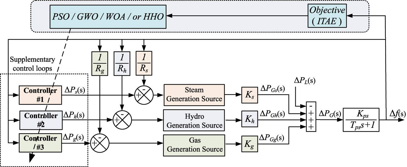
LFC for isolated multi-source power system through bio-inspired algorithms (examined here) optimization. Notation with respect to Figure 1.
4.1 Scenarios examined
In order to examine the system dynamics in terms of transient performance parameters like peak undershoot (U sh ), peak overshoot (O sh ), and settling time (T s ) of the corresponding frequency fluctuations due to a load disturbance, the power system is appropriately modeled and the control strategies are implemented in MATLAB and Simulink environments. The power system model under consideration was used to run a variety of scenarios as shown in Table 1 and the simulation results from each instance are reported next. Each time, the four different bio-inspired algorithms (PSO, GWO, WOA and HHO) were used to evaluate the system’s performance. The same procedure was followed for PI, PID and FOPID controllers. According to Table 1 the following apply:
In scenario 1 a dedicated controller is used for each source, the steam unit is considered reheated and the load disturbance in the area (ΔP L ) is equal to 1 %.
In scenario 2, all the above applies except that the load disturbance is equal to 2 %.
The scenarios of the examined LFC problem.
| Scenario | ΔP L | Controller | GDB (steam) | GRC (steam) | Boiler | GRC (hydro) |
|---|---|---|---|---|---|---|
| 1 | 1 % | Dedicated | – | – | – | – |
| 2 | 2 % | Dedicated | – | – | – | – |
| 3 | 1 % | Dedicated | Yes | Yes | – | – |
| 4 | 1 % | Dedicated | Yes | Yes | Yes | – |
| 5 | 1 % | Dedicated | Yes | Yes | Yes | Yes |
| 6 | 1 % | Common | – | – | – | – |
For the rest of the scenarios, the load disturbance (ΔP L ) is kept equal to 1 %.
Scenario 3 has the characteristics of Scenario 1 and additionally, GRC as well as GDB are considered for the steam unit.
In scenario 4, boiler dynamics are additionally considered for the steam unit.
In scenario 5, GRC for the hydro unit is taken into account.
Finally, Scenario 6 has the characteristics of Scenario 1, except that a common controller was used for all three sources.
It should be noted that the latter scenario is examined for “negative” demonstration purposes i.e. it will be deducted from the results that common controllers (which may be met in some works) are not advised, whereas dedicated controllers for each source are preferable in LFC studies.
4.2 Results and discussion
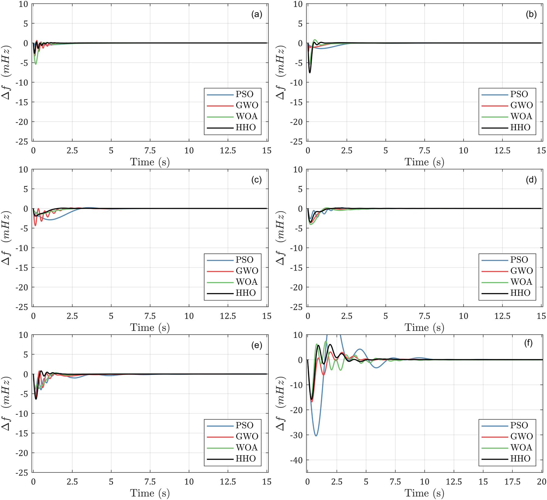
Signals are sampled at 50 ms which is considered a very safe sampling frequency as it is 8–10 times larger than most common industrial sampling equipment while the system’s frequency deviation (Δf) time responses are simulated. The simulations have yielded significant results, which are summarized in Figures 7 –9 and Tables 2 –4. With regard to the PI controller, Table 2 shows that the ITAE for the different scenarios and for the different algorithms are (in descending order) the PSO (deterioration on average 64.4 %), WOA (deterioration on average 38.43 %), GWO (deterioration on average 37.39 %) compared to the HHO. Figure 7 provides a visual representation of the frequency deviation response of the PI controller exhibited by the different optimization algorithms. The figure clearly shows that the HHO produced the smallest undershoot in all examined cases, while the PSO produced the highest overshoot. Notably, the HHO exhibited the shortest settling time and, on average, the PSO reaches stability more slowly. It is also observed that as nonlinearities are added to the system (i.e. scenarios 3, 4), the settling time increases in the cases of GWO, WOA and PSO and decreases in the case of HHO.

System’s frequency deviation time responses using PI controller tuned by PSO, GWO, WOA and HHO, for the different examined operating scenarios (with respect to Table 1): (a) scenario 1, (b) scenario 2, (c) scenario 3, (d) scenario 4, (e) scenario 5 and (f) scenario 6.

System’s frequency deviation time responses using PID controller tuned by PSO, GWO, WOA and HHO, for the different examined operating scenarios (with respect to Table 1): (a) scenario 1, (b) scenario 2, (c) scenario 3, (d) scenario 4, (e) scenario 5 and (f) scenario 6.
System’s frequency deviation time responses using FOPID controller tuned by PSO, GWO, WOA and HHO, for the different examined operating scenarios (with respect to Table 1): (a) scenario 1, (b) scenario 2, (c) scenario 3, (d) scenario 4, (e) scenario 5 and (f) scenario 6.
Frequency deviation dynamic response characteristics and objective function (ITAE) value obtained for the examined scenarios with the PI controller (w.r.t. Figure 7(a)–(f)).
| Scenario | Algorithm | U sh (mHz) | O sh (mHz) | T s (s) | ITAE |
|---|---|---|---|---|---|
| 1 | PSO | −12.546 | 0.2082 | 5.1247 | 0.0123 |
| GWO | −9.7388 | 3.6368 | 4.9761 | 0.0065 | |
| WOA | −9.8325 | 4.1129 | 5.0123 | 0.0076 | |
| HHO | −8.5576 | 3.5991 | 4.0573 | 0.0041 | |
| 2 | PSO | −21.408 | 9.0797 | 4.6844 | 0.0120 |
| GWO | −19.668 | 7.5689 | 4.4985 | 0.0119 | |
| WOA | −15.937 | 4.7697 | 5.1289 | 0.0131 | |
| HHO | −14.329 | 6.9469 | 2.3317 | 0.0048 | |
| 3 | PSO | −8.6347 | 0.9754 | 6.5131 | 0.0246 |
| GWO | −8.7562 | 2.9327 | 4.2799 | 0.0052 | |
| WOA | −8.9297 | 0.2969 | 5.5530 | 0.0059 | |
| HHO | −7.7465 | 2.2223 | 3.4111 | 0.0044 | |
| 4 | PSO | −19.344 | 1.7598 | 6.5131 | 0.0259 |
| GWO | −11.576 | 0.0000 | 4.0744 | 0.0105 | |
| WOA | −10.856 | 6.2879 | 4.1824 | 0.0094 | |
| HHO | −7.2008 | 2.4824 | 3.6622 | 0.0044 | |
| 5 | PSO | −20.023 | 1.4756 | 7.7701 | 0.0243 |
| GWO | −17.789 | 0.0000 | 12.265 | 0.0211 | |
| WOA | −17.267 | 8.3445 | 7.1501 | 0.0184 | |
| HHO | −16.879 | 5.7132 | 7.1479 | 0.0175 | |
| 6 | PSO | −40.374 | 2.9819 | 16.3023 | 0.2198 |
| GWO | −40.162 | 2.7455 | 16.3094 | 0.2198 | |
| WOA | −40.664 | 2.7455 | 16.3089 | 0.2198 | |
| HHO | −40.344 | 3.0482 | 16.2925 | 0.2198 |
-
Bold values show that the proposed algorithm exhibits the lower (better) control variable settling time compared to the other algorithms.
Frequency deviation dynamic response characteristics and objective function (ITAE) value obtained for the examined scenarios with the PID controller (w.r.t. Figure 8(a)–(f)).
| Scenario | Algorithm | U sh (mHz) | O sh (mHz) | T s (s) | ITAE |
|---|---|---|---|---|---|
| 1 | PSO | −3.7502 | 1.4515 | 8.5952 | 0.0057 |
| GWO | −3.5294 | 0.7239 | 1.7821 | 0.0014 | |
| WOA | −3.6071 | 1.4617 | 3.6771 | 0.0016 | |
| HHO | −4.5607 | 0.0000 | 1.6672 | 0.0004 | |
| 2 | PSO | −7.1832 | 1.6832 | 3.4015 | 0.0031 |
| GWO | −7.4689 | 0.0000 | 2.6482 | 0.0011 | |
| WOA | −7.4261 | 0.0000 | 2.7534 | 0.0015 | |
| HHO | −8.3644 | 0.0000 | 2.2176 | 0.0009 | |
| 3 | PSO | −7.9244 | 2.1382 | 9.0737 | 0.0105 |
| GWO | −7.3221 | 3.3802 | 2.5441 | 0.0016 | |
| WOA | −7.8735 | 4.2717 | 3.8373 | 0.0029 | |
| HHO | −5.9023 | 4.3419 | 2.4100 | 0.0013 | |
| 4 | PSO | −6.0132 | 0.5028 | 6.2720 | 0.0026 |
| GWO | −7.8141 | 0.1081 | 3.2710 | 0.0021 | |
| WOA | −6.2040 | 0.3842 | 4.3373 | 0.0038 | |
| HHO | −5.7441 | 0.2943 | 2.9269 | 0.0015 | |
| 5 | PSO | −11.015 | 6.4078 | 3.1847 | 0.0077 |
| GWO | −11.220 | 3.3984 | 2.4221 | 0.0042 | |
| WOA | −10.969 | 4.0601 | 2.2665 | 0.0044 | |
| HHO | −11.349 | 3.2427 | 1.8432 | 0.0041 | |
| 6 | PSO | −16.109 | 10.149 | 4.4525 | 0.0192 |
| GWO | −16.116 | 9.9605 | 4.2669 | 0.0192 | |
| WOA | −16.371 | 9.9699 | 4.2637 | 0.0192 | |
| HHO | −16.112 | 9.9662 | 4.2579 | 0.0192 |
-
Bold values show that the proposed algorithm exhibits the lower (better) control variable settling time compared to the other algorithms.
Frequency deviation dynamic response characteristics and objective function (ITAE) value obtained for the examined scenarios with the FOPID controller (w.r.t. Figure 9(a)–(f)).
| Scenario | Algorithm | U sh (mHz) | O sh (mHz) | T s (s) | ITAE |
|---|---|---|---|---|---|
| 1 | PSO | −1.0006 | 0.0000 | 10.8983 | 0.0017 |
| GWO | −3.3333 | 0.6309 | 2.5590 | 0.0009 | |
| WOA | −5.3510 | 0.0031 | 4.2487 | 0.0018 | |
| HHO | −2.6123 | 0.2964 | 2.5326 | 0.0004 | |
| 2 | PSO | −1.4074 | 0.0015 | 10.0391 | 0.0042 |
| GWO | −2.0917 | 0.0000 | 2.0536 | 0.0011 | |
| WOA | −5.5501 | 0.7854 | 3.6790 | 0.0016 | |
| HHO | −7.5731 | 0.1795 | 0.9630 | 0.0009 | |
| 3 | PSO | −2.8753 | 0.2097 | 6.2292 | 0.0087 |
| GWO | −4.3334 | 0.0000 | 4.9899 | 0.0026 | |
| WOA | −1.4443 | 0.0000 | 4.8059 | 0.0018 | |
| HHO | −1.9043 | 0.0075 | 3.5439 | 0.0009 | |
| 4 | PSO | −2.5274 | 0.0000 | 8.7298 | 0.0029 |
| GWO | −3.5584 | 0.0012 | 4.3072 | 0.0026 | |
| WOA | −4.0511 | 0.1621 | 5.0638 | 0.0036 | |
| HHO | −3.3396 | 0.0092 | 2.6053 | 0.0011 | |
| 5 | PSO | −5.1068 | 0.3342 | 9.7897 | 0.0094 |
| GWO | −5.6807 | 0.6743 | 5.6306 | 0.0042 | |
| WOA | −3.8180 | 0.2504 | 2.8965 | 0.0025 | |
| HHO | −6.3034 | 0.7222 | 1.7236 | 0.0011 | |
| 6 | PSO | −29.625 | 21.011 | 10.2922 | 0.1328 |
| GWO | −16.650 | 0.6169 | 8.2656 | 0.0294 | |
| WOA | −14.987 | 5.7975 | 8.4739 | 0.0716 | |
| HHO | −15.536 | 5.5283 | 7.2841 | 0.0245 |
-
Bold values show that the proposed algorithm exhibits the lower (better) control variable settling time compared to the other algorithms.
With regard to the PID controller, Table 3 shows that the ITAE for the different scenarios and for the different algorithms are (in descending order) the PSO (deterioration on average 68.2 %), WOA (deterioration on average 47.2 %), GWO (deterioration on average 27.4 %) compared to the HHO. Additionally, when comparing the objective functions of the PI and PID controllers, it is evident that the PID controller consistently achieves a lower ITAE in all examined scenarios. This improvement can be attributed to the presence of the differential term in the PID controller, which significantly reduces the settling time. In addition, by observing the Figures 7 and 8, it can be seen that in the case of a PID controller, the undershoot, overshoot and settling time have been significantly reduced. As shown by the PI controller and similarly observed with the PID controller, the maximum settling time in all scenarios is given by PSO and the minimum by HHO.
For the last controller (FOPID) considered for the LFC problem in the examined system, the ITAE value for the different algorithms (in descending order) was obtained to be the PSO (deterioration on average 80.5 %), WOA (deterioration on average 60.5 %), GWO (deterioration on average 47.8 %) compared to the HHO. In the scenarios with non-linearities HHO-FOPID succeeded in giving lower objective function values than HHO-PID: 30.7 %, 26.7 %, 73.2 %, for Scenarios 3, 4 and 5, respectively. The FOPID controller exhibits an additional distinction not present in the other two controllers. In scenario 6, during the optimization process, the algorithms successfully determined distinct gains for each controller, with HHO yielding the most optimal results.
All algorithms successfully found gain values that led the system to stability for all types of controllers. It was observed that the HHO consistently produced the smallest objective function values across all three controllers. Additionally, indicatively for Scenario 5 — which incorporates all the non-linearities — the frequency deviation response of the HHO-FOPID controller showed a shorter settling time (improved by 75.88 % and 6.49 % for the HHO-PI and HHO-PID controllers, respectively) and less overshoot (improved by 87.72 % and 78.13 % for the HHO-PI and HHO-PID controllers, respectively), as depicted in Figures 7 –9. These findings indicate that the HHO algorithm has the potential to be a valuable tool for optimizing gain values for various controllers. It can enhance system performance and stability. However, it is important to acknowledge the challenge of determining the superiority of one algorithm over another, as the no-free-lunch (NFL) theorem clarifies. This theorem states that no single algorithm can effectively solve every problem. Instead, different algorithms are better suited for different problems. In the context of this study, the HHO algorithm demonstrates superiority in solving the single-area multi-source LFC problem, but it may encounter challenges when applied to other types of problems.
5 Further analysis of designed controller robustness
From the comparative procedure carried out in the previous Section, the superiority of the FOPID controller over PI and PID clearly emerged. The further analysis will be performed with the FOPID controller which is tuned with the HHO algorithm. Two different cases were taken into consideration, and simulations were run to demonstrate the performance of the suggested controller. The values of the optimized controller parameters obtained from the simulation are displayed in Table 5.
FOPID controllers’ gains obtained through the HHO for the examined scenarios.
| Scenario | K p | K i | K d | λ | μ | |
|---|---|---|---|---|---|---|
| Steam | ||||||
| 1 | 50.000 | 50.000 | 23.7023 | 0.7657 | 0.9614 | |
| 2 | 36.6839 | 33.5676 | 50.000 | 0.8552 | 0.0231 | |
| 3 | 11.1286 | 31.7419 | −14.8050 | 1.2682 | 2.000 | |
| 4 | 46.3294 | 27.6468 | −18.8350 | 0.6147 | 0.4048 | |
| 5 | 30.2630 | 49.2810 | −2.7367 | 0.7753 | 0.0476 | |
| 6 | 3.6588 | 5.9147 | 1.4939 | 1.2461 | 0.9122 | |
| Hydro | ||||||
| 1 | 29.6143 | 37.6520 | 28.2451 | 0.6992 | 0.0187 | |
| 2 | −46.5612 | −5.8138 | −1.8314 | 1.1364 | 0.9908 | |
| 3 | 49.3488 | 6.3938 | −19.6270 | 1.1183 | 0.9227 | |
| 4 | −2.7089 | 17.1958 | −9.1576 | 0.9767 | 0.8558 | |
| 5 | −21.3082 | 4.8211 | −30.6765 | 1.1435 | 0.1048 | |
| 6 | 3.6588 | 5.9147 | 1.4939 | 1.2461 | 0.9122 | |
| Gas | ||||||
| 1 | 36.7075 | 50.000 | 7.5965 | 0.8614 | 1.1724 | |
| 2 | −24.0074 | 31.8878 | −46.4246 | 0.9431 | 0.5935 | |
| 3 | 50.000 | 50.000 | 50.000 | 0.9139 | 0.9407 | |
| 4 | 44.5391 | 46.5285 | 0.9727 | 27.2651 | 0.7911 | |
| 5 | 50.000 | 48.1202 | 4.9719 | 0.5677 | 1.4062 | |
| 6 | 3.6588 | 5.9147 | 1.4939 | 1.2461 | 0.9122 |
5.1 Random load disturbance
In this examined case, the dynamical load fluctuation of ΔP L is considered to demonstrate the effectiveness of the proposed HHO-FOPID control method. To show the performance robustness of the HHO-FOPID controller at different perturbations compared with other algorithms, a random load disturbance is applied, as shown in Figure 10. The system response oscillations are illustrated in Figure 11 which depicts the frequency deviation response comparison of the three different scenarios (i.e. scenarios 1, 4 and 5) with the HHO-FOPID controller and indicatively the frequency response for Scenario 1 with the four different bio-inspired algorithms.
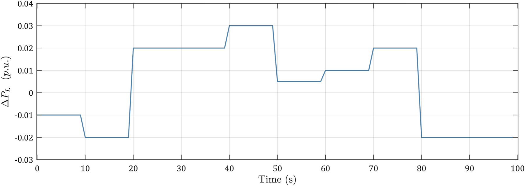
Random load profile.

Frequency deviation response for system load variation as per Figure 10, (a) with the FOPID controller and for scenario 1, (b) with the HHO-FOPID controller for scenarios 1, 4 and 5.
In this case, the frequency deviation response range lied between ±5 mHz for the PSO algorithm, ±3 mHz for WOA, while the corresponding range for the rest of the algorithms was only ±2 mHz. It can be seen that the proposed HHO-FOPID controller continues to provide the best response for random load variation. It provides less steady-state error, faster response, and better damped oscillation than that achieved using other algorithms. By observing Figure 11(a), it can be seen that, at the instant where the maximum overshoot (t = 80 s) and maximum undershoot (t = 40 s) occurred, the load went from the maximum value to the minimum and from the minimum to the maximum, respectively. The remaining peaks of the frequency deviation response appeared whenever the load changed between the other levels.
Based on the analysis of Figure 11(b), it can be inferred that the frequency deviation response range for scenario 1 is ±1 mHz, whereas for the other two scenarios involving non-linearities, the corresponding range is ±6 mHz. Additionally, it was seen that there were “sharp” edges in this plot in scenarios 4 and 5. This can be attributed to the increased complexity of the systems in these Scenarios due to the presence of the GRC, GDB and boiler. As demonstrated in Figure 11, the HHO-FOPID controller was capable of balancing demand and generation even under fast-changing random load conditions.
5.2 Sensitivity analysis
Sensitivity analysis is crucial for proving any controller’s effectiveness. In this subsection, a sensitivity analysis to assess the stability of the suggested approach (HHO-FOPID) is performed. The effects of the variation of the system constants on the dynamic response of the power system are investigated and the obtained results are summarized in Table 6. Each system constant is increased by 20 % of its nominal value, and the effect on system dynamics is examined in terms of transient performance parameters (i.e. peak undershoot U sh , peak overshoot O sh and settling time T s . It is demonstrated that the impact of modifying system constants on the system’s dynamic performance is almost negligible. It can be concluded that the suggested approach is stable under a variety of scenarios and that the controller gains determined under nominal conditions do not need to be changed when a large range of variation is applied to the system constants.
System dynamic performance assessment for 20 % increment of the parameters: T SG , T T , T GH and T w for the proposed HHO-FOPID controller.
| Scenario | Constant varied | HHO | ||
|---|---|---|---|---|
| U sh (mHz) | O sh (mHz) | T s (s) | ||
| 1 | T SG | −2.6238 | 0.2442 | 2.5425 |
| T T | −2.6263 | 0.2527 | 2.5986 | |
| T GH | −2.6237 | 0.2696 | 2.5326 | |
| T w | −2.6236 | 0.2527 | 2.6250 | |
| T CD | −2.5721 | 0.2527 | 2.3672 | |
| 2 | T SG | −7.5731 | 0.1629 | 0.8952 |
| T T | −7.4791 | 0.0723 | 0.9658 | |
| T GH | −7.4797 | 0.1628 | 0.9462 | |
| T w | −7.5567 | 0.1374 | 0.8994 | |
| T CD | −7.5730 | 0.0074 | 0.9523 | |
| 3 | T SG | −1.8831 | 0.0067 | 3.5439 |
| T T | −1.8938 | 0.0068 | 3.5356 | |
| T GH | −1.8830 | 0.0078 | 3.5213 | |
| T w | −1.9112 | 0.0061 | 3.4985 | |
| T CD | −1.9157 | 0.0076 | 3.5157 | |
| 4 | T SG | −3.4482 | 0.0092 | 2.6135 |
| T T | −3.4216 | 0.0082 | 2.6048 | |
| T GH | −3.4325 | 0.0090 | 2.5998 | |
| T w | −3.4572 | 0.0091 | 2.6072 | |
| T CD | −3.4406 | 0.0094 | 2.6198 | |
| 5 | T SG | −6.3112 | 0.7198 | 1.7245 |
| T T | −6.2714 | 0.7197 | 1.7236 | |
| T GH | −6.3454 | 0.6839 | 1.7162 | |
| T w | −6.3792 | 0.6887 | 1.7292 | |
| T CD | −6.3118 | 0.7192 | 1.7189 | |
| 6 | T SG | −15.451 | 5.4597 | 7.3841 |
| T T | −15.538 | 5.5528 | 7.1598 | |
| T GH | −15.534 | 5.4166 | 7.4895 | |
| T w | −15.351 | 5.1875 | 7.4561 | |
| T CD | −15.629 | 5.5284 | 7.3546 | |
6 Conclusions
The current research has explored the LFC characteristics of a power generating system with steam, hydro and gas generation sources, with and without the presence of non-linearities imposed by generation rate constraints, governor dead band and boiler dynamics. The methodology followed for solving this LFC problem was divided into two phases: a controller optimization procedure and an analysis of the proposed controller’s robustness. The system was initially considered with a constant step load variation, and for six different Scenarios. For the purposes of ensuring reliable results, three different controller architectures (PI, PID, and FOPID) were evaluated, and their gains were obtained using various bio-inspired algorithms (PSO, GWO, WOA and HHO). The simulation results indicated that the HHO-FOPID controller exhibited superior performance in terms of power system stability compared to other controllers designed using heuristic algorithms (improved on average by 47.8 %, 80.5 % and 60.5 % for the GWO-, PSO-, and WOA tuned FOPID controllers, respectively). Furthermore, the HHO-FOPID controller yielded the lowest objective function for all examined Scenarios, followed by the HHO-PID (deterioration of 21.62 %) and HHO-PI (deterioration of 84.33 %).
The evaluation and examination of the results demonstrated that the proposed approach provides improved stability in terms of settling time and reduces frequency deviation, resulting in a reduction in peak overshoot and undershoot. In order to ensure the superiority and reliability of the HHO-FOPID controller during the second phase, two separate simulation scenarios were taken into account. In the first case, a random load disturbance was applied and the second case involved a sensitivity analysis. The results of these simulations demonstrated the superior performance of the HHO-FOPID controller in maintaining frequency control in the system, highlighting its effectiveness in maintaining stability in the face of disturbances.
The results presented indicated that the HHO algorithm outperformed all other algorithms across all examined cases. This can be attributed to the HHO algorithm’s ability to update the search agents, which eventually leads to finding the global optimum. HHO can solve constrained problems and maintain its balance between exploitation and exploration. Finally, some suggestions for future actions may include:
The application of the HHO algorithm to LFC problems pertaining to multi-area multi-source systems especially in a deregulated market environment.
The application of the HHO algorithm for solving complex multi-objective optimization problems, such as microgrid energy management problems.
The expansion of the system considered in this study to include the integration of renewable energy sources like PV and wind ones.
-
Author contributions: All the authors have accepted responsibility for the entire content of this submitted manuscript and approved submission.
-
Conflict of interest statement: The authors declare no conflicts of interest regarding this article.
-
Research funding: This research received no specific grant from any funding agency in the public, commercial, or not-for-profit sectors.
Appendix A: System parameters
Nominal system frequency f = 60 Hz.
Power system: K ps = 68.9566, T ps = 11.49 s.
Speed droop regulation: R s = R h = R g = 2.4 Hz/pu MW.
Source participation factors: K s = 0.57143, K h = 0.28571, K g = 0.14286.
Steam unit: T sg = 0.08 s, K sg = 1, T r = 10 s, K r = 0.3, K t = 1, T t = 0.3 s.
Hydro unit: T R = 5 s, T rh = 28.75 s, T gh = 0.2 s, T w = 1 s.
Gas unit: X = 0.6, Y = 1, a = c = 1, b = 0.05, T cr = 0.01 s, T f = 0.23 s, K cd = 1, T cd = 0.2 s.
Governor dead band: N 1 = 0.8, N 2 = −0.2π.
GRC limits (upper/lower) for steam: +10 %/−10 % (or else ±0.0017 pu/s).
GRC limits (upper/lower) for hydro: +270 %/min/−360 %/min (or else +0.045 pu/s and −0.06 pu/s).
Boiler dynamics: K 1 = 0.85, K 2 = 0.095, K 3 = 0.92, K 1B = 0.03, T 1B = 26 s, T 2B = 6.9 s, C B = 200, T D = 0, T fb = 10 s.
References
1. Kundur, P, Balu, NJ, Lauby, MG. Power system stability and control. EPRI power system engineering series. New York: McGraw-Hill Education; 1994.Search in Google Scholar
2. Karnavas, YL, Papadopoulos, DP. AGC for autonomous power system using combined intelligent techniques. Elec Power Syst Res 2002;62:225–39. https://doi.org/10.1016/s0378-7796(02)00082-2.Search in Google Scholar
3. Tungadio, DH, Sun, Y. Load frequency controllers considering renewable energy integration in power system. Energy Rep 2019;5:436–53. https://doi.org/10.1016/j.egyr.2019.04.003.Search in Google Scholar
4. Ranjitha, K, Sivakumar, P, Monica, M. Load frequency control based on an improved chimp optimization algorithm using adaptive weight strategy. COMPEL 2022;41:1618–48. https://doi.org/10.1108/compel-07-2021-0231.Search in Google Scholar
5. Ramakrishna, KSS, Bhatti, TS. Sampled-data automatic load frequency control of a single area power system with multi-source power generation. Elec Power Compon Syst 2007;35:955–80. https://doi.org/10.1080/15325000701199479.Search in Google Scholar
6. Ramakrishna, KSS, Bhatti, TS. Automatic generation control of single area power system with multi-source power generation. Proc Inst Mech Eng A J Power Energy 2008;222:1–11. https://doi.org/10.1243/09576509jpe405.Search in Google Scholar
7. Godara, K, Kumar, N. Frequency analysis of multi-source single area power system using WCA algorithm. In: Proc. of 2021 4th international conference on recent developments in control, automation & power engineering (RDCAPE), Noida, India; 2021:492–6 pp.10.1109/RDCAPE52977.2021.9633690Search in Google Scholar
8. Paliwal, N, Srivastava, L, Pandit, M. Application of grey wolf optimization algorithm for load frequency control in multi-source single area power system. Evol Intell 2022;15:563–84. https://doi.org/10.1007/s12065-020-00530-5.Search in Google Scholar
9. Dash, PM, Mohapatra, SK, Baliarsingh, AK. Tuning of LFC in multi-source electrical power systems implementing novel nature inspired MFO algorithm based controller parameter. In: Proc. of 2020 international conference on computational intelligence for smart power system and sustainable energy (CISPSSE), Keonjhar, India; 2020:1–5 pp.10.1109/CISPSSE49931.2020.9212199Search in Google Scholar
10. Dinakin, DD, Oluseyi, PO. Comparative study of meta-heuristic and classical techniques for automatic generation control of a multi-source single-area hydro-thermal-gas power system. Kufa J Eng 2019;10:151–72. https://doi.org/10.30572/2018/kje/100310.Search in Google Scholar
11. Sivalingam, R, Chinnamuthu, S, Dash, SS. A hybrid stochastic fractal search and local unimodal sampling based multistage pdf plus (1+pi) controller for automatic generation control of power systems. J Franklin Inst 2017;354:4762–83. https://doi.org/10.1016/j.jfranklin.2017.05.038.Search in Google Scholar
12. Tavakoli, M, Pouresmaeil, E, Adabi, J, Godina, R, Catalão, JPS. Load-frequency control in a multi-source power system connected to wind farms through multi terminal HVDC systems. Comput Oper Res 2018;96:305–15. https://doi.org/10.1016/j.cor.2018.03.002.Search in Google Scholar
13. Mohanty, B, Panda, S, Hota, PK. Controller parameters tuning of differential evolution algorithm and its application to load frequency control of multi-source power system. Int J Electr Power Energy Syst 2014;54:77–85. https://doi.org/10.1016/j.ijepes.2013.06.029.Search in Google Scholar
14. Celik, E, Ozturk, N, Arya, Y, Ocak, C. (1+PD)-PID cascade controller design for performance betterment of load frequency control in diverse electric power systems. Neural Comput Appl 2021;33:15433–56. https://doi.org/10.1007/s00521-021-06168-3.Search in Google Scholar
15. Arya, Y. AGC performance enrichment of multi-source hydrothermal gas power systems using new optimized FOFPID controller and redox flow batteries. Energy 2017;127:704–15. https://doi.org/10.1016/j.energy.2017.03.129.Search in Google Scholar
16. Padhy, S, Panda, S, Mahapatra, S. A modified GWO technique based cascade PI-PD controller for AGC of power systems in presence of plug in electric vehicles. Eng Sci Technol Int J 2017;20:427–42. https://doi.org/10.1016/j.jestch.2017.03.004.Search in Google Scholar
17. Padhy, S, Panda, S. A hybrid stochastic fractal search and pattern search technique based cascade PI-PD controller for automatic generation control of multi-source power systems in presence of plug in electric vehicles. CAAI Trans Intell Technol 2017;2:12–25. https://doi.org/10.1016/j.trit.2017.01.002.Search in Google Scholar
18. Barakat, M, Donkol, A, Hamed, HFA, Salama, GM. Harris hawks-based optimization algorithm for automatic LFC of the interconnected power system using PD-PI cascade control. J Electr Eng Technol 2021;16:1845–65. https://doi.org/10.1007/s42835-021-00729-1.Search in Google Scholar
19. Elaziz, MA, Heidari, AA, Fujita, H, Moayedi, H. A competitive chain-based Harris hawks Optimizer for global optimization and multi-level image thresholding problems. Appl Soft Comput 2020;95:106347. https://doi.org/10.1016/j.asoc.2020.106347.Search in Google Scholar
20. Sahu, J, Debnath, MK, Mohanty, PK, Sahu, BK. Application of Harris hawks optimization to solve LFC issues in solar based unified system. In: Proc. of 2021 1st Odisha international conference on electrical power engineering, communication and computing technology (ODICON), Bhubaneswar, India; 2021:1–5 pp.10.1109/ODICON50556.2021.9429015Search in Google Scholar
21. Ramoji, SK, Saikia, LC, Dekaraja, B, Behera, MK, Bhagat, SK, Babu, NR. Optimal unified frequency and voltage control of multi-area multi-source power system using the cascaded PIDN-TIDF controller. In: Proc. of 2020 IEEE 17th India council international conference (INDICON), New Delhi, India; 2020:1–6 pp.10.1109/INDICON49873.2020.9342228Search in Google Scholar
22. Sobhy, MA, Ezzat, M, Hasanien, HM, Abdelaziz, AY. Harris hawks algorithm for automatic generation control of interconnected power systems. In: Proc. of 2019 21st international middle east power systems conference (MEPCON), Cairo, Egypt; 2019:575–82 pp.10.1109/MEPCON47431.2019.9007968Search in Google Scholar
23. Karnavas, YL, Nivolianiti, E. Load frequency control in multi-source power generation systems using Harris hawks optimization algorithm. In: 2022 international conference on communications, information, electronic and energy systems (CIEES); 2022:1–6 pp.10.1109/CIEES55704.2022.9990646Search in Google Scholar
24. Annamraju, A, Nandiraju, S. Robust frequency control in a renewable penetrated power system: an adaptive fractional order-fuzzy approach. Prot Control Mod Power Syst 2019;4:16. https://doi.org/10.1186/s41601-019-0130-8.Search in Google Scholar
25. Karnavas, YL. On the optimal load frequency control of an interconnected hydro electric power system using genetic algorithms. In: Proc. of the 6th IASTED international conference on European power and energy systems (EuroPES 2006), Rhodes, Greece; 2006:526–31 pp.Search in Google Scholar
26. Karnavas, YL, Dedousis, KS. Overall performance evaluation of evolutionary designed conventional AGC controllers for interconnected electric power system studies in a deregulated market environment. Int J Eng Sci Technol 2010;2:150–66.10.4314/ijest.v2i3.59185Search in Google Scholar
27. Karnavas, YL, Nivolianiti, E. Optimal load frequency control of a hybrid electric shipboard microgrid using jellyfish search optimization algorithm. Appl Sci 2023;13:6128. https://doi.org/10.3390/app13106128.Search in Google Scholar
28. Heidari, AA, Mirjalili, S, Faris, H, Aljarah, I, Mafarja, M, Chen, H. Harris hawks optimization: algorithm and applications. Future Generat Comput Syst 2019;97:849–72. https://doi.org/10.1016/j.future.2019.02.028.Search in Google Scholar
29. Shehab, M, Mashal, I, Momani, Z, Shambour, MKY, Al-Badareen, A, Al-Dabet, S, et al.. Harris hawks optimization algorithm: variants and applications. Arch Comput Methods Eng 2022;29:5579–603. https://doi.org/10.1007/s11831-022-09780-1.Search in Google Scholar
© 2023 the author(s), published by De Gruyter, Berlin/Boston
This work is licensed under the Creative Commons Attribution 4.0 International License.
Articles in the same Issue
- Frontmatter
- Review
- Grid integration of wind farms and the interconnection requirements for the U.S. grid
- Research Articles
- Islanding detection and power quality disturbance classification in multi DG based microgrid using down sampling empirical mode decomposition and multilayer neural network
- Research on image acquisition and contour extraction algorithm of partial discharge in oil
- Experimental validation of non-dual adaptive controller based DSTATCOM for power quality enhancement
- An experimental and numerical study to evaluate performance parameters of GIS circuit breaker during low current interruption
- Development of an H ∞ controller for a microgrid using LabVIEW
- Bayesian optimization of multi-layer perceptron models for power distribution system state estimation
- Design and analysis of solar hybrid battery swapping station
- Traceability analysis of distributed new energy system access to green power based on blockchain consensus algorithm
- Distributed new energy system access based on blockchain Consensus Algorithm
- A new control method for the steadiness of electric vehicles with 2-motor in rear and front wheels
- Harris hawks optimization algorithm for load frequency control of isolated multi-source power generating systems