A novel transient search optimization for optimal allocation of multiple distributed generator in the radial electrical distribution network
-
 and
and


Abstract
Most of the generated electricity is lost in power loss while transmitting and distributing it to the consumer end. The power losses occurring in the distribution network cause deviation in voltage and lower stability due to increased load demand. The integration of multiple Distributed Generation (DG) will enable the existing radial electrical distribution network efficient by minimizing the power losses and improving the voltage profile. Metaheuristic optimization techniques provide a favorable solution for optimal location and sizing of DG in the distribution network. A novel modern metaheuristic Transient Search Optimization (TSO) algorithm, inspired by the electrical network’s transient response of storage components implemented in the proposed work. The TSO formulated optimal DGs allocation to minimize total active power loss, voltage deviation and enhance voltage stability index as minimization optimization problem satisfying various equality and inequality constraints. The installation of multiple DG units at unity, fixed, and optimal power factors were examined. The TSO algorithm’s effectiveness was tested on standard IEEE 33-bus and 69-bus radial distribution networks, including various operating events developed in the form of single and multi-objective fitness functions. The active power loss reduced to 94.29 and 94.71% for IEEE 33 and 69 bus distribution systems. The obtained results trustworthiness is confirmed by comparison with well-known optimization methods like Genetic Algorithm (GA), Particle Swarm Optimization (PSO), combined GA/PSO, Teaching Learning Based Algorithm (TLBO), Swine influenza model-based optimization with quarantine (SIMBO-Q), Multi-Objective Harris Hawks optimizer (MOHHO) and other provided in the literature. The presented numerical studies represent the usefulness and out-performance of the proposed TSO algorithm due to its exploration and exploitation optimization mechanisms for the DG allocation problem meticulously.
Nomenclature
- Parameters
- b
-
Branch number
- N b
-
Number of branches
- I b
-
The absolute magnitude of current streaming inside the branch
- R b
-
Resistance of branch b
- N m
-
Total number of bus
- V m
-
The magnitude of voltage for bus m
- m
-
Bus number
- V std
-
The standard value of system voltage
- a
-
Starting bus
- c
-
Ending bus
- lb
-
The lower bound of the search region
- P c
-
Active power
- Q c
-
Reactive power
- R ac
-
Resistance connecting buses a, and c
- X ac
-
Reactance connecting buses a, and c
- N DG
-
Number of DG
- P DG, n
-
DG’s active power
- Q DG, n
-
DG’s reactive power
- P D, m
-
Active power demand
- Q D, m
-
Reactive power demand
- f d
-
Damped resonant frequency
- X b
-
Branch reactance
- V min, m
-
The minimum value of bus m voltage
- V max, m
-
The maximum value of bus m voltage
- I max, b
-
Maximum branch current
- P DG min, m
-
Minimum active power limits of DG
- P DG max, m
-
Maximum active power limits of DG
- Q DG min, m
-
Minimum reactive power limits
- Q DG max, m
-
Maximum reactive power limits
- PF DG min, m
-
Minimum power factor limit of DG
- r 1 , r 2 , and r 3
-
Random aggregates scattered uniformly ϵ [0, 1]
- T
-
Random coefficient
- C 1
-
Random coefficient
- X J
-
Current location of search agents
- X J *
-
Best location of search agents
- z
-
Changing variable that varies from 2 to 0
- k
-
Constant number (k = 0, 1, 2, …)
- J max
-
Total number of iterations
- X min
-
Minimum quantity of the problem variables
- X max
-
The maximum quantity of the problem variables
- ub
-
Upper bound of the search region
- O
-
Computational complexity
- N
-
Search agent
- D
-
Dimension
- Ir
-
Independent run
- P C
-
Penalty factor
- F C
-
Constraint functions
- s
-
Size of DG
- l
-
Location of DG
- x(t)
-
Either the capacitor voltage v(t) of the RC circuit or an inductor current i(t) of the RL circuit,
- rand
-
A random number
- PF DG, max, m
-
Maximum power factor limit of DG
- DGLocation, min
-
Minimum bus location for placement of DG
- DGLocation, max
-
Maximum bus location for placement of DG
- d
-
Dimension of DG
- t
-
Time
- τ
-
Circuit time constant
- K
-
Constant dependent on the initial value of x(0) and the final result value is x(∞)
- α
-
Damping coefficient
- ω 0
-
Resonant frequency
- Acronyms
- REDN
-
Radial electrical distribution system
- TSO
-
Transient search optimization
- DG
-
Distributed generation
- TAPL
-
Total active power loss
- TAPLR
-
Total active power loss reduction
- VD
-
Voltage deviation
- PF
-
Power factor
- MOF
-
Multi objective function
- VSI
-
Voltage stability index
- VP
-
Voltage profile
- OLSDG
-
Optimal location and size of DG
- GA
-
Genetic algorithm
- PSO
-
Particle swarm optimization
- CS
-
Cuckoo search
- GSA
-
Gravitational search algorithm
- SO
-
Single-objective
- QOTLBO
-
Quasi-oppositional teaching-learning based optimization
- SIMBO-Q
-
Swine influenza model-based optimization with quarantine
- HHO
-
Harris hawks optimizer
- IHHO
-
Improved harris hawks optimizer
- UPF
-
Unity power factor
- OPF
-
Optimal power factor
- BSOA
-
Backtracking search optimization algorithm
- OBF
-
Objective function
- IVD
-
Improvement in voltage deviation
- IVSI
-
Improvement in voltage stability index
- WOA
-
Whale optimization algorithm
- BFOA
-
Bacterial foraging optimization algorithm
- SKHA
-
Stud krill herd algorithm
- TLBO
-
Teaching-learning based optimization
- FPF
-
Fixed power factor
- FF
-
Fitness function
- HS
-
Harmony search
- MO
-
Multi-objective
- QOSIMBO-Q
-
Quasi-oppositional swine influenza model-based optimization with quarantine
1 Introduction
1.1 Motivation
Electricity demand is rising worldwide day by day, establishing the necessity of massive amounts of power production, which require either building a new power plant or expanding existing ones to meet the increased load demand. The generated electricity from the power plant arrived at the consumer end through transportation over a long distance. A significant portion of electricity is lost as power loss while transmitting it. In a developed country like the USA, the power loss is 6% after having a well-established distribution network; for developing countries like India, the power loss is up to 38% of total generated electricity [1]. A major portion of electricity is generated from conventional coal-based sources, which increases the carbon emission in the atmosphere; according to the Paris agreement, carbon emissions are mitigated while fostering sustainable development [2]. Figure 1 shows the power loss situation worldwide, illustrating the need to reduce its amount with alternative solutions. The power losses in 54 percent of countries range from 10 to 72 percent of total electricity generation. One percentage point reduction in power losses will cause 1.6 to 5.4 percent of fossil plants to withdraw from 2 to 72 percent for respective loss rates [3].

Power loss mapping worldwide.
The distribution network has higher total active power loss (TAPL), high voltage deviation (VD), and low voltage stability index (VSI) relative to the transmission network due to the increased R/X ratio and radial structure. The promising solution for the high power loss while meeting the increasing electricity demand is the deployment of distributed generation (DG) in the radial electrical distribution system (REDN) to strengthen the power value chain system [4]. The small-scale generation varies from a few hundred kW to MW, located onsite or close to the load center available for integration into the distribution network known as distributed generation [5]. It is the cost-effective and trending solution for electrical utility because of reducing the high investment, operating cost, and construction time of building a new power plant besides expanding the existing distribution network [6]. The DG can be selected according to the location and availability since it can be either conventional or green energy source types. DG technologies, including internal combustion engines, combustion turbines, micro-turbines, wind turbines, photovoltaic, biomass, cells, geothermal, limited hydropower, are explicitly considered. Besides, DG technologies primarily derived from renewable energy sources such as solar and wind reduced carbon emission [7]. The inaccurate allotment of DGs would lead to an enormous power loss, reverse power flow, overall voltage drops, and substandard stability of the system. Therefore, the optimal location and size of DG (OLSDG) need to be evaluated to standardize technological and economic strengths in REDN configuration. After integrating DG units with proper allocation, TAPL decreased, voltage profile (VP) enhanced, resulting in the better performance of the REDN [8]. The mixed-integer nonlinear problem of OLSDG needs to be solved by metaheuristics optimization techniques for reducing power loss and maximizing the efficiency of REDN by improving the VP due to its specific advantages for computing elevated dimensional problem with fast convergence rate and global optimal search strength [9].
1.2 Literature review
Attributable to DG’s tremendous advantages, the DG allocation issue has been a relevant topic of study for the last decade. Experts have ascertained and proposed numerous methods for optimally allocating DG units within the distribution system. The allocation of DG is determined by different analytical methods based on sensitivity factors [10]. A new voltage stability index-based optimal integration is performed for single and multiple DG in the distribution system to minimize the power loss and improvement in the voltage profile [11, 12]. A simple iterative analytical method was applied for the DG allocation problem by modifying the original method using iteration for optimal sizing and location [13]. It is easy to implement the DG allocation problem with sensitivity approach-based methods; however, it takes a longer time hence becomes complicated for multiple DG types, including multi-objective analysis.
Artificial intelligence-based approaches are usually robust and hold the superior potential to obtain an optimal solution. Some approaches might fail through localized optimality for complicated and high-dimensional problems and consume substantial computational time and slower convergence speed. The allocation of DG is done by stochastic methods based on artificial intelligence influenced by natural inspiration; it can be categorized as bio-inspiration and physical inspiration. The bio-inspired algorithms are either swarm-based or evolutionary-based, whereas scientific laws and equations intrinsically motivate the physical-inspiration algorithms. Figure 2 represents several metaheuristic optimization algorithms utilized for the DG allocation problem. An evolutionary-based algorithm such as genetic algorithm (GA) and swarm-based particle swarm optimization (PSO) was implemented for OLSDG for different load models in the distribution network [14, 15]. Artificial bee colony algorithm applied for DG allocation to reduce the TAPL with improved VP [16]. The wolf’s hunting behaviors influenced DG with different types allocated by the grey wolf optimization method in many distribution systems to reduce total power loss as the primary objective [17]. This study [18] proposed a metaheuristic optimization cuckoo search (CS) to obtain the OLSDG for loss minimization. The physical inspiration-based gravitational search algorithm (GSA) is utilized to lessen the TAPL and boost VP in REDN [19].

Year-wise optimization algorithm for DG allocation.
To surmount prematurity and diminish the stochastic method’s search region, a combination with other approaches considered. For DG allocation, a hybrid meta-heuristic algorithm is proposed, combining the phasor particle swarm optimization and the gravitational search algorithm to minimize energy loss and maximization of profit for the distribution system uncertain modeling of solar PV, and wind-based DG applied for DG allocation [20]. In this study, optimal planning of the OLSDG using harmony search (HS) based hybrid technique was revealed by combining GA and adaptive PSO for a multi-objective fitness function [21]. In many studies, the OLSDG is determined by different optimization methods; a combined GA and PSO approach is provided to trace the OLSDG in the REDN, where GA is adopted to scrutinize DG unit positions PSO implemented to optimize their sizes. The purpose of this analysis stood to depreciate the actual TAPL, enhance VP, and improve the distribution system’s voltage stability [22]. Furthermore, the challenge of DG allocation was solved by hybridizing the analytical and swarm based method (AM-PSO), under which the sizes of DG measured by the analytical method and their optimal positions, are obtained according to PSO leading to lower power loss of REDN [23], even if hybrid methods usually have a superior solution range compared to a particular approach, can encounter implementation complications and sluggish convergence rate due to complicated nature and multiple tuning parameters [24].
The problem of OLSDG was tackled using single as well as multi-objective (MO) optimization modes. One objective function involved optimizing the single-objective (SO) optimization problem, reducing the TAPL, VD, and maximizing VSI as the sole objective function of this category. In another way, more than one objective function should be optimized simultaneously in the MO problem. Metaheuristic optimization methodologies have been popularly employed for the OLSDG on together SO and MO concerns. A variety of nature-inspired optimization approaches have previously been used for SO optimization in the OLSDG Problem, such as backtracking search optimization algorithm (BSOA) [25], bacterial foraging optimization algorithm (BFOA) [26], stud krill herd algorithm SKHA [27], and whale optimization algorithm WOA [28]. On the different side, the MO problem employed to deal with the DGs allocation based on two methodologies. A weighting sum approach for individual objective functions used to optimize three objective functions, namely TAPL, VD, and VSI, using Teaching-learning based optimization (TLBO) and Quasi-oppositional teaching-learning based optimization (QOTLBO) [29], swine influenza model-based optimization with quarantine (SIMBO-Q), improved Quasi-oppositional swine influenza model-based optimization with quarantine (QOSIMBO-Q) [30], and Harris hawks optimizer (HHO), and improved harris hawks optimizer (IHHO) [31]. The optimal DG with a smaller size has less installation cost making REDN more economical with introducing minimum complexity [32]. The power factor (PF) control DG units active and reactive power injection into the distribution network. Therefore, specific and unspecified DG power factor values for the allocation problem are considered and optimized.
The literature has revealed that there are few physical-based metaheuristic optimizations applied for optimal allocation of DG. Therefore, in the presented work, applying a new metaheuristic transient search optimization (TSO) algorithm has been intimated with a transient response from electrical circuits, including energy storage components (inductor and capacitor), is executed. A single DG installation is not enough for an extensive distribution network consisting of several loads, buses, and other components. Single DG with a high power-rating will not be a feasible solution as it will make the distribution network more complex, meeting the load growth requirement, so the installation of multiple DG is advantageous over a single DG.
1.3 Contribution and paper organization
This study’s novelty persisted in determining the OLSDG problem in REDN using a new, recently developed modern physical-based metaheuristic optimization algorithm focused on the transient action of electric circuits known as TSO. In the TSO, fewer numbers of parameters need to be tuned compared to other metaheuristic optimization techniques. The main benefits of the TSO are its flexibility and optimization mechanisms. The TSO obtained the global minima with faster convergence and better accuracy in minimum iterations to solve the OLSDG problem for all events considered. TSO’s outstanding exploration ability due to its decay oscillation around the final best solution provides the better optimal solution.
The TSO formulated to allocate DGs to minimize TAPL, VD and enhance VSI through single and multi-objective optimization problems for the different events considered. The integration of multiple DG units with unity, fixed, and optimal power factors have been analyzed. The proposed TSO algorithm’s validity was tested with various operating events on standard IEEE 33-bus and 69-bus REDN. The trustworthiness of the results obtained is confirmed by comparison with the other optimization methods provided in the literature.
The structure of the paper is as follows: Section 2 mathematically formulates the OLSDG problem. Section 3 discusses in-depth the proposed TSO algorithm. Section 4 outlines the TSO’s successful implementation for the DG Allocation Problem in Section 5, followed by the simulation findings in Section 5. The conclusions are eventually provided in Section 6.
2 Problem formulation
This analysis aims to determine the OLSDG while following all operating system restrictions to decrease the TAPL, VD and enhance the VSI in the REDN. In the next subsections, three objective functions were developed mathematically.
2.1 Total active power loss (TAPL)
The higher TAPL come on first priority due to the REDN’s radial structure, so it is necessary to reduce the TAPL. The overall active power losses are calculated in the distribution system using the branch-current loss formula given in Eq. (1).
Where b represents the corresponding branch number in REDN, N b denotes the cumulative number of branches, I b is the absolute magnitude of current streaming inside the branch, and R b demonstrates the resistance of branch b.
2.2 Voltage deviation (VD)
The cumulative combined voltage deviation VD means the distribution system’s voltage output level and its distance from the specified standard voltage magnitude. The following Eq. (2) is applied to estimate it accurately.
Where m represents the specific bus number, N m denotes the total number of buses, V m indicates the magnitude of voltage for bus m, V std symbolizes the standard value of system voltage.
2.3 Voltage stability index (VSI)
The VSI was developed to analyze REDN’s capability for voltage control within the tolerable range [33]. The primary intention resides in optimizing the lowest VSI of the distribution system.
Where a and c stand for the starting and ending bus. P c , Q c signify active besides reactive power at the ending bus; moreover, R ac and X ac imply the resistance along with reactance connecting buses a, and c.
2.4 Single-objective (SO)
For a single objective, the DG allocation problem is to reduce the active power loss (OBF1) successively, depreciate the voltage deviation (OBF2), and maximize the VSI (OBF3). Each objective reported as follows:
2.5 Multi-objective (MO)
The three SO functions mentioned are incorporated to obtain a MO optimization function [34]. The SO function is scaled by its base value and associated with the weighting coefficients to form the MO function. The definitive multi-objective function of the problem is as follows in Eq. (7).
Since equal importance is given for all the objective functions, so the weighting factor is assigned the equal weight in MO for the DG allocation optimization problem [35].
2.6 Constraints
All SO and MO functions established are restricted to enforcing limits of equity and inequalities constraints.
2.6.1 Power balance constraints
The REDN’s active and reactive powers must be kept under control to prevent reverse power flow as follows:
Where NDG represents the number of DG allocated. PDG,n, Q DG, n signifies DG’s active as well as reactive power of DG. P D,m , Q D,m epitomizes active and reactive power demand by the loads. RPL is the reactive power loss, and X b demonstrates the branch reactance.
2.6.2 Voltage limits
Within the lower and upper boundaries, the bus voltage magnitude will be managed as follows:
Where Vmin, m, Vmax, m is the minimum and maximum value of bus m voltage.
2.6.3 Thermal limit
The current that passes within a branch should not exceed its thermal limit. The same as described by:
Where Imax,b is maximum branch current.
2.6.4 DG capacity limits
DG unit power outputs vary as follows from maximum to minimum levels of active power, reactive power, and power factor.
Where PDGmin,m, PDGmax,m corresponds to the minimum and maximum active power limits of DG. QDG min, m, QDG max, m symbolizes minimum and maximum reactive power limits, PFDG,min,m, PFDG,max,m, signify minimum and maximum power factor limit of DG.
2.6.5 DG location limits
The allocation of DG units is limited by the minimum and maximum number of buses.
Where DGLocation,min, DGLocation,max is minimum and maximum bus location for placement of DG.
3 Transient search optimization (TSO)
This algorithm is stimulated by the transient responses of switched electric circuits requiring storage components such as inductance plus capacitance. The exploring and exploiting capability of the TSO algorithm were tested by optimizing several mathematical benchmark functions. Many engineering design optimization problems, solved and findings are correlated with the new optimization algorithms [36].
3.1 Background
The circuits’ complete response with resistive and power storage variables such as capacitors, inductors, or mutually involves a transient response coupled with a steady-state response. The transitioning of the first and second-order circuits cannot automatically shift the mechanism into the following constant condition, in which a condenser or inductor takes time to be charged or discharged before the steady-state value is estimated.
3.1.1 First-order response
where t signifies the time, x(t) denotes either the capacitor voltage v(t) of the RC circuit or an inductor current i(t) of the RL circuit, τ symbolize the circuit time constant, where τ = RC of the RC circuit and τ = L/R of the RL circuit, K is a constant dependent on the initial value of x(0) and the final result value is x(∞).
3.1.2 Second-order response
Where α and ω 0 represent the damping coefficient and the resonant frequency, f d means the damped resonant frequency, B1 and B2 are constants. The under-damped reaction happens when α < ω0 induces the RLC circuit’s transient response to damped oscillations. The second-order response is assumed underdamped.
3.2 Modeling of TSO
3.2.1 Initialization
Search-agents randomly initialize within the below and uppermost bounds of the search domain.
First, the search-agents initialization is generated randomly as in
where lb, ub correspond to the lower and upper bound of the search region, rand implies a random number dispersed consistently.
3.2.2 Exploration and exploitation
Exploration seeks the best solution, while exploitation is finding a steady-state solution or the best one. TSO’s discovery activity was improved by the oscillations of second-order circuits around the null point. Consequently, the exploitation of TSO is facilitated by the exponential decay in electric circuits of the first-order discharge of storage components. The computational modeling of the TSO algorithm exploitation and exploration showed by Eq. (21), incited by the total response (transient and steady-state) of the first and second-order electrical network by Eq. (23).
The random quantity r 1 utilized to coordinate within the exploration (r 1 ≥ 0.5) and exploitation (r 1 < 0.5) of the TSO algorithm. T and C 1 are random coefficients, r 1 , r 2 , and r 3 are random aggregates scattered uniformly ϵ [0, 1]. X J , X J * signifies the location of search agents and best location respectively, it resembles the ultimate state of the electrical circuit. In this paper, the parameter of the proposed TSO algorithm to allocated DG is given in Table 1
Parameter of TSO.
| Parameter | Value |
|---|---|
| Search agent (N) | 30 |
| Maximum iteration (Jmax) | 100 |
| Independent run (Ir) | 30 |
In the TSO algorithm exploitation procedure performed once T > 0, (high to low response transition) while the exploration process executed when T < 0, (low to high transition); the equilibrium between the exploration and exploitation rule effectuated by the coefficient T, which ϵ [−2, 2].
Where z signifies a changing variable that varies from 2 to 0 as in Eq. (24), k denotes a constant number (k = 0, 1, 2, …), and Jmax illustrates the total number of iterations.
3.2.3 Updating
The solution’s updating will take place according to the following relation amid TSO algorithm optimization with upper and lower limits.
Where, Xmin, Xmax characterizes the minimum and maximum quantity of the problem variables.
The best location of the decision variable is obtained based on the computational complexity O of the proposed algorithm, which depends on the product of the different number of search agents N, dimension D.
and maximum iteration Jmax according to the following equation for the minimization problem amid a single independent run of TSO
For a fixed number of independent runs Ir, the best solution will be achieved according to the following Eq. (28).
3.3 Application of TSO for OLSDG
The flowchart of TSO is presented in Figure 3. The application of the TSO algorithm implemented for DG allocation sequentially given by following steps:
Enter load and line data of distribution system, define fitness function FF with penalty factor P C for different constraint functions F C .
Initialise the TSO algorithm’s parameter and decision variables for DG allocation like the number of randomly generated search agents, the maximum number of iteration, and independent runs.
Where s is the size of DG, l is the location of DG, and d is the dimension of DG d = 1, 2, 3.
The power factors should be considered as decision variables to be calculated when installing DGs with various power factors. The DG with optimal power factor capable of providing both active and reactive power to achieve the best results for minimization of the fitness function. This DG type requires a particular intervention. The power factor of DG is calculated as follows for optimization of DG sizing.
Where c is a conversion coefficient, PFDG power factor of DG unit.

Flowchart of TSO.
The power factor of DG is calculated as follow:
In DG with unity power factor (UPF) PFDG = 1 p.u.
In DG with fixed power factor (FPF) PFDG = 0.95 p.u.
In DG with optimal power factor (OPF) PFDG = x p.u., x € rand(0, 1).
The value of x is obtained by implementing the TSO algorithm for the single and multi-objective fitness function. After selecting a specified DG type, perform power flow and calculate each search agent’s fitness function’s value.
Check the constraints limit during each iteration and update the solution within the lower and upper bound of the decision variable according to Eq. (25).
Store the best solution and modify this solution according to Eq. (27) based on the exploration and exploitation process by updating the parameter coefficients T, r 1, and C 1 of the TSO algorithm.
Check the boundary condition for size and location and update it according to Eq. (28).
Compare solution after every iteration; the new solution would replace the old solution if it had a minimum value of the objective function; otherwise, it will be discarded, maintaining the old solution as the best solution.
If termination criteria (J > Jmax) are achieved, record the so far best solution, and increment independent run of the algorithm for the new locations and sizes of DG.
After a certain number of independent runs, select the best solution with a minimum fitness function value.
Record the best solution and run power flow again for assessment of results.
4 Results and discussion
The distribution system includes many buses and with highly resistive branches that constitute radial structures for an unbalanced load and operate differently compared to the transmission system. Therefore, the conventional load flow methods are not accurate in the distribution system. Therefore backward forward sweep load flow algorithm is adopted for analyzing the considered test distribution system from [37]. In this work, IEEE-33 and 69 REDN taken to implement TSO for the OLSDG problem. All the line and load data for both test REDN are taken from [38]. The TSO algorithm was implemented through the four considered events shown in Table 2.
Objective distribution for optimization of events.
| Event | TAPL | VD | VSI | Optimization |
|---|---|---|---|---|
| 1 |

|

|
|
SO |
| 2 |
|
|
|
SO |
| 3 |
|
|
|
SO |
| 4 |
|
|
|
MO |
In each event, the following four distinct cases are utilized to evaluate DG allocation in Table 3.
The cases considered under each event.
| Cases | Description |
|---|---|
| Base case | No DG |
| Case 1 | Three DGs with unity power factor (UPF) |
| Case 2 | Three DGs with fixed power factor (FPF) |
| Case 3 | Three DGs with optimal power factor (OPF) |
The APL, VD, and VSI are evaluated with the integration of DG with various power factors. All the simulation results are tabulated and compared with previously applied metaheuristic optimization techniques.
4.1 IEEE-33 BUS REDN
The TSO algorithm is utilized on the IEEE-33 REDN primarily. The single line diagram is given in Figure 4. The 33 buses are connected by 32 branches in a radial structure. Bus 1 is slack bus supplies the losses into the network after receiving the power from centralized generation. The base voltage and power ratings are 12.66 kV and 100 MVA, respectively. The total active and reactive power load is 3715 kW and 2300 kVAr, respectively. In the base case, after performing the load flow, the preliminary magnitude of objectives found 211 kW TAPL, 0.1338 p.u. VD and 1.4988 p.u. 1/VSI rating.
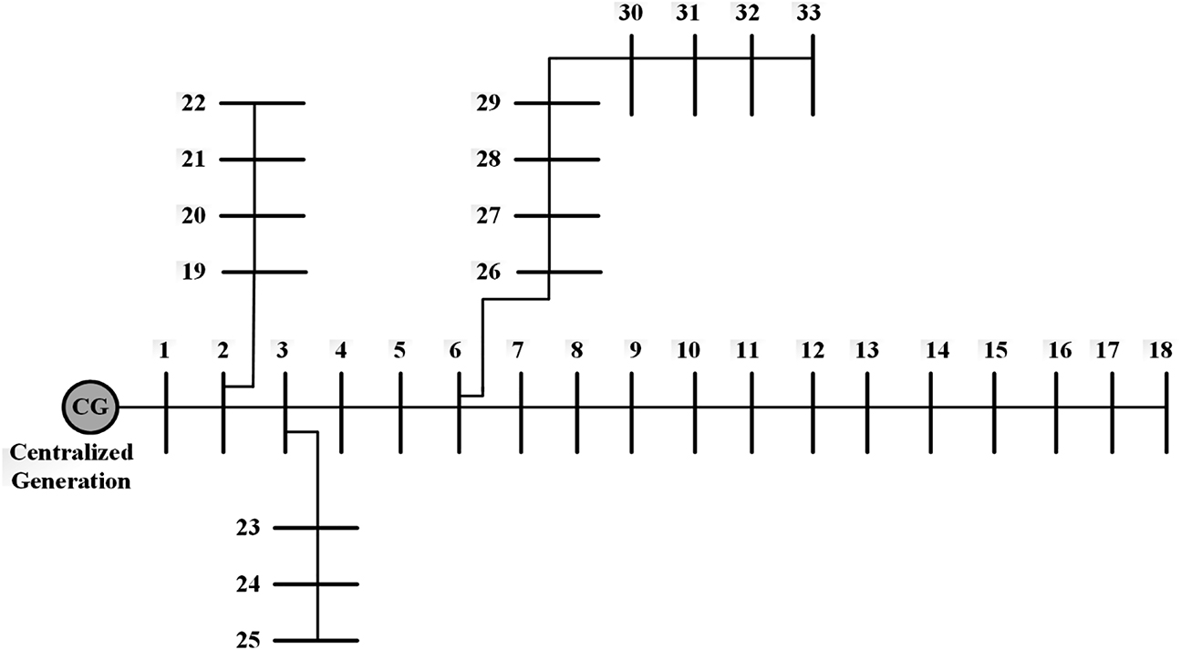
Single line layout of IEEE-33 REDN.
4.1.1 Event-1
In event 1, the TSO applied for the OLSDG problem with the singular target of minimizing the TAPL. Table 4 describes the outcomes for all instances provided by the TSO and other optimization methods for direct comparison on a common benchmark.
Comparative result summary for event-1.
| Method | Optimal DG | TAPL (kW) | TAPLR (%) | ||
|---|---|---|---|---|---|
| Location (Bus) | Size (kW) | PF (p.u.) | |||
| Base case | – | – | – | 211 | – |
| Case 1 | |||||
| Fuzzy-IAS [39] | 32 | 2071 | 1.0 | 117.36 | 42.45 |
| 30 | 1113.8 | 1.0 | |||
| 31 | 150.3 | 1.0 | |||
| BSOA [25] | 13 | 632 | 1.0 | 89.05 | 57.76 |
| 28 | 486 | 1.0 | |||
| 31 | 550 | 1.0 | |||
| LSF [40] | 18 | 720 | 1.0 | 85.07 | 59.72 |
| 33 | 810 | 1.0 | |||
| 25 | 900 | 1.0 | |||
| TLBO [29] | 10 | 824.6 | 1.0 | 75.54 | 64.20 |
| 24 | 1031.1 | 1.0 | |||
| 31 | 886.2 | 1.0 | |||
| KHA [41] | 13 | 810.7 | 1.0 | 75.41 | 64.26 |
| 25 | 836.8 | 1.0 | |||
| 30 | 841 | 1.0 | |||
| QOTLBO [29] | 12 | 880.8 | 1.0 | 74.10 | 64.88 |
| 24 | 1059.2 | 1.0 | |||
| 29 | 1071.4 | 1.0 | |||
| BFOA [26] | 14 | 779 | 1.0 | 73.53 | 65.14 |
| 25 | 880 | 1.0 | |||
| 30 | 1083 | 1.0 | |||
| SIMBO-Q [30] | 14 | 763.8 | 1.0 | 73.4 | 65.21 |
| 24 | 1041.5 | 1.0 | |||
| 29 | 1135.2 | 1.0 | |||
| QOSIMBO-Q [30] | 14 | 770.8 | 1.0 | 72.79 | 65.49 |
| 24 | 1096.5 | 1.0 | |||
| 30 | 1065.5 | 1.0 | |||
| TSO | 14 | 771.54 | 1.0 | 72.79 | 65.50 |
| 24 | 1103.65 | 1.0 | |||
| 30 | 1064.57 | 1.0 | |||
| Case 2 | |||||
| SIMBO-Q [30] | 13 | 887.5 | 0.95 | 29 | 86.26 |
| 24 | 1085.3 | 0.95 | |||
| 30 | 1309.2 | 0.95 | |||
| QOSIMBO-Q [30] | 13 | 830.3 | 0.95 | 28.5 | 86.49 |
| 24 | 1123.9 | 0.95 | |||
| 30 | 1239.8 | 0.95 | |||
| HHO [31] | 13 | 871.34 | 0.95 | 29.71 | 85.92 |
| 24 | 1326.76 | 0.95 | |||
| 30 | 1076.05 | 0.95 | |||
| IHHO [31] | 14 | 793.81 | 0.95 | 28.5 | 86.49 |
| 24 | 1132.44 | 0.95 | |||
| 30 | 1257.76 | 0.95 | |||
| Proposed (TSO) | 13 | 833.22 | 0.95 | 28.5 | 86.49 |
| 24 | 1083.4 | 0.95 | |||
| 30 | 1250 | 0.95 | |||
| Case 3 | |||||
| BSOA [25] | 13 | 698 | 0.86 | 29.65 | 85.97 |
| 29 | 402 | 0.71 | |||
| 31 | 658 | 0.70 | |||
| BFOA [26] | 14 | 600 | 0.89 | 27.5 | 86.97 |
| 25 | 598 | 0.83 | |||
| 30 | 934 | 0.88 | |||
| HHO [31] | 12 | 913.05 | 0.85 | 14.94 | 92.92 |
| 24 | 882.86 | 0.82 | |||
| 30 | 1079.05 | 0.83 | |||
| Proposed (TSO) | 14 | 753.75 | 0.88 | 12.03 | 94.29 |
| 24 | 1142.74 | 0.93 | |||
| 30 | 1047.51 | 0.73 | |||
For case 1, when DGs are allocated on bus locations 14th, 24th, and 30th with capacity 771.54, 1103.65, and 1064.57 kW, the TAPL decreased to 72.79 kW by TSO. From comparison with other methods, it is found that TSO and QOSIMBO-Q offer the minimum value of TAPL. The TSO algorithm reached the global solution with only two tunning variables with a simplified approach, whereas the QOSIMBO-Q has a larger number of tunning variables to achieve the same global solution, which makes the process much complicated.
For case 2, when DGs were allocated 13th, 24th, and 30th with size 833.22, 1083.4, and 1250 kW. The TSO produced the minimum TAPL of 28.5 kW, which is comparable to QOSIMBO-Q and IHHO methods, but the total DG size is lower compared to all the methods listed, provided a cost-effective solution.
In case 3, the TAPL obtained by TSO was 12.03 kW, power loss reduced to 94.29% with respect to the base case, when no DGs were installed, which is lower to compare all other methods. The optimal locations were 14th, 24th, and 30th, with size 753.75 kW at 0.88 PF, 1142.74 kW at 0.93 PF, and 1047.51 kW at 0.73 PF, respectively.
It was observed from summarized results that the percentages of total active power loss reduction (TAPLR) were 65.50, 86.49, and 94.29% for cases 1, 2, and 3, respectively. In case 3, power loss reduction was the largest against cases 1 and 2. It suggested that DG units performing superior with OPF significantly impacted the reduction in power loss. The convergence characteristic is seen in Figure 5 showed that for cases 1, 2, and 3, the optimal minima found before 10, 80, and 20 iterations. The REDN voltage profile improved after DG allocation for the specified cases clearly displayed in Figure 6.

Convergence characteristics for active power loss as a single objective.

Voltage profile for single objective as power loss.
4.1.2 Event-2
Table 5 describes the disclosures obtained by TSO and other approaches for event 2, with the aim of minimizing the VD accompanying all cases.
Comparative result summary for event-2.
| Method | Optimal DG | VD (p.u.) | IVD (%) | ||
|---|---|---|---|---|---|
| Location (Bus) | Size (kW) | PF (p.u.) | |||
| Base case | – | – | – | 0.1338 | – |
| Case 1 | |||||
| QOTLBO [29] | 14 | 1074.4 | 1.0 | 0.00086 | 99.35 |
| 27 | 1200 | 1.0 | |||
| 33 | 1200 | 1.0 | |||
| QOSIMBO-Q [29] | 7 | 1490.3 | 1.0 | 0.00066 | 99.50 |
| 13 | 958 | 1.0 | |||
| 31 | 1271.4 | 1.0 | |||
| SFSA [42] | 7 | 1487.1 | 1.0 | 0.0006597 | 99.50 |
| 13 | 960.4 | 1.0 | |||
| 31 | 1263.8 | 1.0 | |||
| SOS [43] | 14 | 909.9 | 1.0 | 0.0006579 | 99.50 |
| 31 | 1299.7 | 1.0 | |||
| 7 | 1500 | 1.0 | |||
| QOCSOS [43] | 31 | 1259.9 | 1.0 | 0.0006571 | 99.50 |
| 13 | 955.1 | 1.0 | |||
| 7 | 1500 | 1.0 | |||
| Proposed (TSO) | 11 | 1533.75 | 1.0 | 0.00047 | 99.64 |
| 24 | 1629.61 | 1.0 | |||
| 32 | 1437.89 | 1.0 | |||
| Case 2 | |||||
| Proposed TSO | 12 | 1085.39 | 0.95 | 0.00045 | 99.66 |
| 23 | 1627.06 | 0.95 | |||
| 29 | 1392.46 | 0.95 | |||
| Case 3 | |||||
| Proposed TSO | 13 | 835.11 | 0.89 | 0.00025 | 99.81 |
| 24 | 1112.39 | 0.94 | |||
| 30 | 1367.97 | 0.89 | |||
In the base case, the VD is 0.1338 p.u., the TSO estimated a VD of 0.00047 p.u. when DGs size 1533.75, 1629.61, and 1437.89 kW are placed on bus locations 11th, 24th, and 32nd of test REDN for case 1. It was most minuscule VD compared to other optimization techniques with an improvement of 99.64%.
The injection of reactive power along with active power TSO acquired further minimum VD of magnitude 0.00045 p.u. for case 2 after DG allocation; however, in case 3, TSO’s outcome exhibited the magnitude of VD was 0.00025 p.u., leading to a reduction of 99.81% with reference to base case due to an optimal balance of adequate active and reactive power injection with additional optimization of power factor taken as a decision variable.
In the three cases of DG power factor, the VD value observed in case 3 was significantly smaller than that reported in the remaining cases. It explicates that the differences in all bus voltages of REDN are substantially minimum, resulting in an enhanced individual voltage of all buses with the smaller amount of current flow in the branches of REDN when DG with an OPF is integrated into REDN. Figure 7 displays the TSO convergence graph, intimates a faster convergence curve for case 3 before the 90th iteration, whereas the global solution for case 1 and 2 obtained after 90th and before the 100th iteration.

Convergence characteristics for voltage deviation as a single objective.
4.1.3 Event-3
In event 3, TSO is applied to solve the OLSDG problem for maximizing VSI under SO optimization. The results obtained from TSO and other methods were tabulated for cases 1, 2, and 3 in Table 6.
Comparative result summary for event-3.
| Method | Optimal DG | 1/VSI (p.u.) | IVSI (%) | ||
|---|---|---|---|---|---|
| Location (Bus) | Size (kW) | PF (p.u.) | |||
| Base case | – | – | – | 1.4988 | – |
| Case 1 | |||||
| QOTLBO [29] | 6 | 1199.8 | 1.0 | 1.0397 | 30.63 |
| 11 | 1200 | 1.0 | |||
| 29 | 1198.3 | 1.0 | |||
| QOSIMBO-Q [30] | 7 | 1500 | 1.0 | 1.0292 | 31.33 |
| 13 | 719.9 | 1.0 | |||
| 31 | 1500 | 1.0 | |||
| SFSA [42] | 12 | 1499.7 | 1.0 | 1.0294 | 31.31 |
| 25 | 713.6 | 1.0 | |||
| 31 | 1499.9 | 1.0 | |||
| SOS [32] | 12 | 1500 | 1.0 | 1.0293 | 31.32 |
| 25 | 715.1 | 1.0 | |||
| 31 | 1500 | 1.0 | |||
| QOCSOS [32] | 12 | 1500 | 1.0 | 1.0293 | 31.32 |
| 31 | 1500 | 1.0 | |||
| 25 | 715.1 | 1.0 | |||
| Proposed (TSO) | 14 | 1600 | 1.0 | 1.0228 | 31.75 |
| 24 | 1700 | 1.0 | |||
| 33 | 1500 | 1.0 | |||
| Case 2 | |||||
| QOSIMBO-Q [23] | 29 | 1578.9 | 0.95 | 1.0234 | 31.71 |
| 24 | 1337.5 | 0.95 | |||
| 13 | 998.4 | 0.95 | |||
| SFSA [31] | 10 | 1319.8 | 0.95 | 1.0223 | 31.79 |
| 24 | 1573.1 | 0.95 | |||
| 30 | 1476.4 | 0.95 | |||
| SOS [32] | 24 | 1578.9 | 0.95 | 1.0223 | 31.79 |
| 30 | 1574.2 | 0.95 | |||
| 11 | 1216.2 | 0.95 | |||
| QOCSOS [32] | 12 | 1578.9 | 0.95 | 1.0223 | 31.79 |
| 31 | 1574.2 | 0.95 | |||
| 25 | 1216.2 | 0.95 | |||
| Proposed (TSO) | 9 | 1600 | 0.95 | 1.0197 | 31.96 |
| 24 | 2000 | 0.95 | |||
| 30 | 1500 | 0.95 | |||
| Case 3 | |||||
| SFSA [31] | 13 | 1052.7 | 0.85 | 1.0221 | 31.80 |
| 24 | 1694.2 | 0.84 | |||
| 29 | 1622.1 | 0.85 | |||
| SOS [32] | 11 | 1134.6 | 0.88 | 1.0221 | 31.80 |
| 30 | 1519.1 | 0.88 | |||
| 24 | 1715.4 | 0.87 | |||
| QOCSOS [32] | 12 | 1140.6 | 0.89 | 1.0221 | 31.80 |
| 30 | 1542.8 | 0.87 | |||
| 24 | 1685.9 | 0.88 | |||
| Proposed (TSO) | 8 | 1591.49 | 0.8 | 1.0185 | 32.04 |
| 24 | 1492.02 | 0.93 | |||
| 29 | 1989.37 | 0.89 | |||
In the base case, the value of 1/VSI is 1.4988 p.u. In case 1, TSO attained the magnitude of 1.0228 p.u. for 1/VSI superior to other methods with an improvement in voltage stability index (IVSI) of 31.75% after installation of DGs on bus locations 14th, 24th, and 33rd with sizes 1600, 1700, and 1500 kW, respectively.
For case 2, TSO obtained the 1/VSI of 1.0197 p.u, with IVSI of 31.96% highest among all optimization techniques. The optimal DGs sizes are 1600, 200, and 1500 kW integrated on bus locations ninth, 24th, and 30th respectively of the REDN.
The 1/VSI had a value of 1.0185 p.u. in case 3 with IVSI of 32.04% when DGs are installed on bus locations eighth, 24th, and 29th with sizes 1591.49 kW at 0.8 PF, 1492.02 kW at 0.93 PF, and 1989.37 kW at 0.89 PF, respectively.
The drop in 1/VSI from case 3 was the most enormous relative to cases 1 and 2. It has been shown that DG units with the OPF increased the VSI resulting in high stability and eliminate the voltage collapse situation of REDN with the addition of increased capability for mitigating the voltage stability problems during operation. Figure 8 displays TSO convergence curves for all cases subject to 1/VSI minimization. The case 3 convergence was obtained after the 80th iteration when global minima found, whereas in cases 1 and 2, faster convergence grasped before the 10th iteration only.

Convergence characteristics for voltage stability index as a single objective.
4.1.4 Event-4
TSO augmented for MO optimization in event 4 after adapting three SO (TAPL, VD, and VSI) by weighted sum scaling approach. Table 7 demonstrates the findings obtained by TSO and other approaches with all cases listed.
Comparative result summary for event-4.
| Method | Optimal DG | TAPL (kW) | VD (p.u.) | VSI (p.u.) | MOF (p.u.) | ||
|---|---|---|---|---|---|---|---|
| Location (Bus) | Size (kW) | PF (p.u.) | |||||
| Base case | – | – | – | 211 | 0.1338 | 0.6672 | 0.9999 |
| Case 1 | |||||||
| GA [22] | 11 | 1500 | 1.0 | 106.3 | 0.0407 | 0.949 | 0.4987 |
| 29 | 422.8 | 1.0 | |||||
| 30 | 1071.4 | 1.0 | |||||
| PSO [16] | 8 | 1176.8 | 1.0 | 105.3 | 0.0335 | 0.9255 | 0.4852 |
| 13 | 981.6 | 1.0 | |||||
| 32 | 829.7 | 1.0 | |||||
| GA/PSO [16] | 11 | 925 | 1.0 | 103.4 | 0.0124 | 0.9508 | 0.4239 |
| 16 | 863 | 1.0 | |||||
| 32 | 1200 | 1.0 | |||||
| GA/IWD [44] | 11 | 1221.4 | 1.0 | 110.51 | 0.0069 | 0.9523 | 0.4211 |
| 16 | 683.3 | 1.0 | |||||
| 32 | 1213.5 | 1.0 | |||||
| TLBO [23] | 12 | 1182.6 | 1.0 | 124.7 | 0.0011 | 0.9503 | 0.4294 |
| 18 | 1191.3 | 1.0 | |||||
| 30 | 1186.3 | 1.0 | |||||
| QOTLBO [23] | 13 | 1083.4 | 1.0 | 103.4 | 0.0011 | 0.9530 | 0.3955 |
| 26 | 1187.6 | 1.0 | |||||
| 30 | 1199.2 | 1.0 | |||||
| TM [45] | 15 | 719.9 | 1.0 | 102.30 | 0.0040 | 0.9371 | 0.4048 |
| 26 | 719.9 | 1.0 | |||||
| 33 | 1439.7 | 1.0 | |||||
| MOTA [45] | 7 | 980 | 1.0 | 96.30 | 0.0014 | 0.9551 | 0.3846 |
| 14 | 960 | 1.0 | |||||
| 30 | 1340 | 1.0 | |||||
| SIMBO-Q [24] | 13 | 1400 | 1.0 | 104.3 | 0.0011 | 0.9615 | 0.3948 |
| 24 | 919.8 | 1.0 | |||||
| 31 | 1400 | 1.0 | |||||
| QOSIMBO-Q [30] | 12 | 1436.8 | 1.0 | 101.9 | 0.0009 | 0.9669 | 0.3893 |
| 25 | 826.2 | 1.0 | |||||
| 31 | 1443.3 | 1.0 | |||||
| MOIHHO [25] | 14 | 1223 | 1.0 | 92.25 | 0.0019 | 0.9580 | 0.3788 |
| 24 | 1144 | 1.0 | |||||
| 31 | 1290 | 1.0 | |||||
| Proposed (TSO) | 12 | 1337.19 | 1.0 | 89.31 | 0.0020 | 0.9416 | 0.3786 |
| 24 | 1185.23 | 1.0 | |||||
| 30 | 1336.75 | 1.0 | |||||
| Case 2 | |||||||
| SIMBO-Q [23] | 30 | 1443 | 0.95 | 32.4 | 0.0003 | 0.977 | 0.2768 |
| 13 | 943 | 0.95 | |||||
| 24 | 1327 | 0.95 | |||||
| QOSIMBO-Q [23] | 30 | 1419 | 0.95 | 31.7 | 0.0003 | 0.977 | 0.2757 |
| 24 | 1392 | 0.95 | |||||
| 13 | 898 | 0.95 | |||||
| MOHHO [25] | 13 | 1008 | 0.95 | 31.4 | 0.0005 | 0.976 | 0.2759 |
| 25 | 910 | 0.95 | |||||
| 30 | 1334 | 0.95 | |||||
| TSO | 14 | 914.44 | 0.95 | 31.06 | 0.0003 | 0.9765 | 0.2748 |
| 24 | 1148.50 | 0.95 | |||||
| 30 | 1431.16 | 0.95 | |||||
| Case 3 | |||||||
| QOSIMBO-Q [23] | 30 | 951 | 0.88 | 18.8 | 0.0005 | 0.978 | 0.2558 |
| 24 | 786 | 0.87 | |||||
| 13 | 1381 | 0.86 | |||||
| TSO | 12 | 932.13 | 0.85 | 14.94 | 0.0003 | 0.9767 | 0.2495 |
| 24 | 1053.96 | 0.84 | |||||
| 30 | 1140.43 | 0.82 | |||||
TSO delivered a MOF 0.3786 p.u. The corresponding magnitudes for TAPL of 88.68 kW, VD of 0.0023 p.u., and a VSI value of 0.9416 p.u. after integration of DG on bus locations 12th, 24th, and 30th with size 1337.19, 1185.23, and 1336.75 kW, respectively. The TAPL from the TSO has a minimum magnitude compared to other algorithms available in the literature. The value of the multi-objective function (MOF) found minimum for TSO when compared with final outcomes of other optimization techniques on a common standard.
In case 2, TSO offered the best results as a MOF of magnitude 0.2748 p.u. the corresponding values of TAPL, VD and VSI are 31.06 kW, 0.0003 p.u., and 0.976 p.u., respectively. The TSO provided the minimum TAPL, VD and VSI is equal to the MOHHO method and comparable to SIMBO-Q and QOSIMBO-Q methods, but overall MOF is lower for TSO compared to other techniques. The optimal bus locations are 14th, 24th, and 30th, with sizes 914.44, 1148.50, and 1431.16 kW, respectively.
Concerning case 3, the MOF further reduced to 0.2495 p.u. the TAPL, VD, and VSI values achieved through TSO are 14.64 kW, 0.0003 p.u., and 0.9767 p.u., sequentially. The optimal bus locations are 14th, 24th, and 30th, with DG, sizes 932.13 kW at 0.85 PF, 1053.96 kW at 0.84 PF, and 1140.43 kW at 0.82 PF, respectively.
Overall, the effectiveness of results is based on the MOF value for all cases. TSO has a smaller MOF magnitude from cases 1–3, respectively, among all optimization algorithms. The case 3 presented the minimum outcomes for all the subsequent objectives as related to cases 1 and 2. From results within the three operational conditions of DG units, it demonstrated a tremendous increase in all three goals, including TAPL, VD, and VSI, while coupling DG with OPF in case 3. Figure 9 demonstrates the convergence characteristics of TSO in event 4; case 1 converged before the 70th iteration while case 2 obtained global minima within the 10th iteration. The case 3 obtained minimum value compared to other cases before the 50th iteration on a scale of 100 iterations.
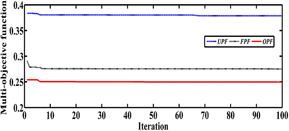
Convergence characteristics as a multi-objective function.
Figures 10 and 11 represent the voltage and VSI profile of the IEEE-33 REDN considering all cases. The case 3 showed a vital transformation with enhanced magnitudes of bus voltages and VSI resultant in a flexible and resilient distribution network.

Voltage profile for multi-objective.

VSI at buses for multi-objective optimization.
4.2 IEEE-69 REDN
This section addresses the IEEE-69 bus medium-scale REDN findings obtained by the implementation of the proposed TSO algorithm. The single-line layout of the test distribution is shown in Figure 12. Except bus 1, all others are load buses, which are the possible location for DG allocation. The base voltage and power ratings are 12.66 kV and 10 MVA, respectively. The total active and reactive power load is 3.8 MW and 2.69 MVAr, respectively. Before adding DG modules, the system’s TAPL, VD, and 1/VSI values were 225 kW, 0.0994 p.u., and 1.4636 p.u., respectively.

Single line layout of IEEE-69 REDN.
4.2.1 Event-1
In event 1, it discusses only the goal of that the TAPL minimization. The TSO simulation results and additional techniques for all cases are addressed in Table 8.
Comparative result summary for event-1.
| Method | Optimal DG | TAPL (kW) | TAPLR (%) | ||
|---|---|---|---|---|---|
| Location (Bus) | Size (kW) | PF (p.u.) | |||
| Base case | – | – | – | 225 | – |
| Case 1 | |||||
| GAPSO [16] | 63 | 884.9 | 1.0 | 81.1 | 63.96 |
| 61 | 1196 | 1.0 | |||
| 27 | 910.5 | 1.0 | |||
| BFOA [26] | 27 | 295.4 | 1.0 | 75.23 | 66.56 |
| 65 | 446 | 1.0 | |||
| 61 | 1345.1 | 1.0 | |||
| TLBO [23] | 15 | 591.9 | 1.0 | 72.41 | 67.82 |
| 61 | 818.8 | 1.0 | |||
| 63 | 900.3 | 1.0 | |||
| QOTLBO [23] | 18 | 533.4 | 1.0 | 71.63 | 68.16 |
| 61 | 1198.6 | 1.0 | |||
| 63 | 567.2 | 1.0 | |||
| SIMBO-Q [24] | 9 | 618.9 | 1.0 | 71.3 | 68.31 |
| 17 | 529.7 | 1.0 | |||
| 61 | 1500 | 1.0 | |||
| QOSIMBO-Q [24] | 9 | 833.6 | 1.0 | 71 | 68.44 |
| 18 | 451.1 | 1.0 | |||
| 61 | 1500 | 1.0 | |||
| Proposed (TSO) | 9 | 825.09 | 1.0 | 70.25 | 68.77 |
| 22 | 405.14 | 1.0 | |||
| 61 | 1650.10 | 1.0 | |||
| Case 2 | |||||
| SIMBO-Q [24] | 19 | 565.6 | 0.95 | 23.1 | 89.73 |
| 61 | 1500 | 0.95 | |||
| 64 | 422 | 0.95 | |||
| QOSIMBO-Q [24] | 17 | 582.8 | 0.95 | 22.8 | 89.86 |
| 61 | 1500 | 0.95 | |||
| 64 | 427.2 | 0.95 | |||
| HHO [25] | 16 | 702.8 | 0.95 | 22.85 | 89.84 |
| 50 | 286.6 | 0.95 | |||
| 61 | 1890.9 | 0.95 | |||
| Proposed (TSO) | 11 | 352.63 | 0.95 | 21.13 | 90.61 |
| 18 | 500.56 | 0.95 | |||
| 61 | 1877.57 | 0.95 | |||
| Case 3 | |||||
| Proposed (TSO) | 12 | 697.35 | 0.80 | 11.89 | 94.71 |
| 59 | 846.39 | 0.91 | |||
| 61 | 1064.60 | 0.81 | |||
In case 1, the DGs are placed on bus locations 9th, 22nd, and 61st with sizes 825.09, 405.14, and 1650.10 kW, respectively, the TAPL reduced to 70.25 kW, which is minimum among all methods listed.
The TSO reduced TAPL 21.13 kW after allocation of DGs on bus locations 11th, 18th, and 61st with rating 352.63, 500.56, and 1877.57 kW, respectively at 0.95 PF in case 2. The RTAPL obtained the 90.61% maximum compared to outcomes found from SIMBO-Q, QOSIMBO-Q, and HHO.
In case 3, the TAPL reduced to 11.89 kW after placement of DGs on bus locations 9th, 59th, and 61st with size 697.35 kW at 0.8 PF, 846.39 kW at 0.91 PF, and 1064.60 kW at 0.81 PF, respectively.
The TSO decreased the TAPL equal to 70.25, 21.13, and 11.89 kW, respectively, heading to a TAPLR of 68.78, 90.61, and 94.71% for cases 1, 2, and 3 individually. The case 3 gives the most economical TAPL across the three events, indicating the most significant effect on TAPLR while DG with OPF is allocated. The convergence curve of case 3 found global minima after the 90th iteration, whereas case 1 and 2 converged quickly within the 80th and 50th iteration, correlating the findings mentioned above as seen in Figure 13. Owing to the decline of the TAPL, the voltage profile improved, as exhibited in Figure 14. Due to the injected active and reactive power, the voltage profile’s substantial improvement is recognized at the optimal PF, nearly comparable to that given by the 0.95 PF for the same reason.

Convergence characteristics for power loss as a single objective.

Voltage profile for single objective as power loss.
4.2.2 Event-2
The solutions found by TSO and other methods for the three cases of DG in event 2 are reviewed in Table 9.
Comparative Result summary for event-2.
| Method | Optimal DG | VD (p.u.) | IVD (%) | ||
|---|---|---|---|---|---|
| Location (Bus) | Size (kW) | PF (p.u.) | |||
| Base case | – | – | – | 0.0993 | – |
| Case 1 | |||||
| QOTLBO [23] | 13 | 1176.4 | 1.0 | 0.00022 | 99.77 |
| 60 | 1117.7 | 1.0 | |||
| 62 | 1196.2 | 1.0 | |||
| QOSIMBO-Q [24] | 14 | 877.7 | 1.0 | 0.000198 | 99.80 |
| 57 | 1155.9 | 1.0 | |||
| 63 | 1491.4 | 1.0 | |||
| Proposed (TSO) | 20 | 597.82 | 1.0 | 0.000190 | 99.80 |
| 55 | 1154.54 | 1.0 | |||
| 63 | 1937.80 | 1.0 | |||
| Case 2 | |||||
| QOSIMBO-Q [24] | 63 | 1578.9 | 0.95 | 0.00022 | 99.77 |
| 56 | 1326.3 | 0.95 | |||
| 17 | 512.7 | 0.95 | |||
| Proposed (TSO) | 9 | 692.55 | 0.95 | 0.00014 | 99.85 |
| 18 | 547.36 | 0.95 | |||
| 62 | 1899.49 | 0.95 | |||
| Case 3 | |||||
| Proposed (TSO) | 6 | 400 | 0.70 | 0.00025 | 99.74 |
| 13 | 841.41 | 0.75 | |||
| 62 | 1441.38 | 0.70 | |||
A VD of 0.000190 p.u. has been recognized in case 1 by TSO. This value remained smaller, corresponded to 0.00022 p.u. (99.80% IVD), QOTLBO, and 0.000198 p.u. QOSIMBO-Q.
For case 2, TSO achieved the tiniest value of VD of 0.00014 p.u. (reduction of 99.85%) compared to the QOSIMBO- Q 0.00022 p.u. (99.77% IVD).
The VD achieved by TSO in case 3 was 0.00025 p.u., which is equivalent to an IVD of 99.74%. The VD mentioned in case 2 was significantly superior amongst all cases. It pointed out that when DG units with 0.95 PF allocated on bus locations 9th, 18th, and 62nd with sizes 692.55, 547.36, and 1899.49 kW, respectively. The VD of REDN extensively improved. Figure 15. illustrates clearly that the convergence curve for case 1 had a faster convergence steep towards global minima compared to case 2 and 3; however, all the curves reached global minima before the 90th iteration obtained optimal solutions.

Convergence characteristics for voltage deviation as a single objective.
4.2.3 Event-3
In event 3, TSO was utilized to solve the problem of OLSDG to optimize the VSI as a SO optimization. In Table 10, the outcomes realized from TSO and other methods reported for all cases. For case 1, the TSO has the same value of 1/VSI (1.0235 p.u.) as obtained by QOTLBO and QOCSOS; however, the total DG size obtained from TSO is less than QOCSOS and slightly more compared to QOTLBO.
Comparative result summary for event-3.
| Method | Optimal DG | 1/VSI (p.u.) | IVSI (%) | ||
|---|---|---|---|---|---|
| Location (Bus) | Size (kW) | PF (p.u.) | |||
| Base case | – | – | – | 1.4615 | – |
| Case 1 | |||||
| QOTLBO [23] | 22 | 1193.1 | 1.0 | 1.0235 | 30.06 |
| 61 | 1196.7 | 1.0 | |||
| 62 | 1191.4 | 1.0 | |||
| QOCSOS [43] | 62 | 2000 | 1.0 | 1.0235 | 30.06 |
| 9 | 1425 | 1.0 | |||
| 21 | 374 | 1.0 | |||
| Proposed (TSO) | 20 | 800 | 1.0 | 1.0235 | 30.06 |
| 61 | 931.77 | 1.0 | |||
| 64 | 2000 | 1.0 | |||
| Case 2 | |||||
| QOSIMBO-Q [24] | 12 | 1212.3 | 0.95 | 1.0233 | 30.08 |
| 61 | 1578.9 | 0.95 | |||
| 55 | 1208.6 | 0.95 | |||
| Proposed (TSO) | 12 | 943.28 | 0.95 | 1.0233 | 30.08 |
| 55 | 1127.47 | 0.95 | |||
| 65 | 1886.75 | 0.95 | |||
| Case 3 | |||||
| SFSA [42] | 18 | 1262 | 0.44 | 1.0061 | 30.62 |
| 50 | 896.6 | 0.49 | |||
| 61 | 2494.3 | 0.55 | |||
| QOCSOS [32] | 62 | 2422.5 | 0.56 | 1.0061 | 30.62 |
| 14 | 1273.5 | 0.44 | |||
| 49 | 964.1 | 0.40 | |||
| Proposed (TSO) | 12 | 1702 | 0.80 | 1.0061 | 30.62 |
| 50 | 1134.7 | 0.80 | |||
| 63 | 1418.3 | 0.70 | |||
For the smaller optimal DGs size allocation on bus locations 12th, 55th, and 65th of distribution network, the TSO found the 1/VSI value 1.0233 p.u. same obtained from QOSIMBO-Q with relatively larger DGs size in case 2.
The TSO has found 1/VSI values of 1.0153 p.u. for case 3 equal to QOCSOS and SFSA, when DGs are integrated on bus locations 12th, 50th, and 63rd different from the previously obtained bus locations. The Total DG size is minimum for TSO compared to QOCSOS and SFSA for the same value of 1/VSI, resulting in cost-effective and economical for the distribution network operator.
The improvement is 30.06, 30.08, and 30.62% in cases 1–3, respectively, since the TSO has given the same 1/VSI value as other methods but with new optimal bus locations and minimum total DGs size, validating proposed TSO performance most accepted compared to other methods. Figure 16 shows the convergence curve of all considered cases with global minima obtained from the TSO algorithm.

Convergence characteristics for voltage stability index as a single objective.
4.2.4 Event-4
In event 4, a MOF was adopted for the OLSDG problem considering TAPL, VD, and VSI simultaneously. The results gained from TSO were distinguished with other approaches, accessed in Table 11.
Comparative result summary for event-4.
| Method | Optimal DG | TAPL (kW) | VD (p.u.) | VSI (p.u.) | MOF (p.u.) | ||
|---|---|---|---|---|---|---|---|
| Location (Bus) | Size (kW) | PF (p.u.) | |||||
| Base case | – | – | – | 225 | 0.0993 | 0.6842 | 0.9999 |
| Case 1 | |||||||
| GA [16] | 21 | 929.7 | 1.0 | 89 | 0.0012 | 0.9705 | 0.3668 |
| 62 | 1075.2 | 1.0 | |||||
| 64 | 984.8 | 1.0 | |||||
| PSO [16] | 17 | 992.5 | 1.0 | 83.2 | 0.0049 | 0.9676 | 0.3713 |
| 61 | 1199.8 | 1.0 | |||||
| 63 | 795.6 | 1.0 | |||||
| GA/PSO [16] | 21 | 910.5 | 1.0 | 81.1 | 0.0031 | 0.9768 | 0.3601 |
| 61 | 1192.6 | 1.0 | |||||
| 63 | 884.9 | 1.0 | |||||
| GA/IWD [44] | 20 | 911.5 | 1.0 | 80.91 | 0.0029 | 0.9814 | 0.3580 |
| 61 | 1392.6 | 1.0 | |||||
| 64 | 805.9 | 1.0 | |||||
| TLBO [23] | 13 | 1013.4 | 1.0 | 82.2 | 0.0008 | 0.9745 | 0.3546 |
| 61 | 990.1 | 1.0 | |||||
| 62 | 1160.1 | 1.0 | |||||
| QOTLBO [23] | 15 | 811.4 | 1.0 | 80.6 | 0.0007 | 0.9769 | 0.3513 |
| 61 | 1147.0 | 1.0 | |||||
| 63 | 1002.2 | 1.0 | |||||
| SIMBO-Q [24] | 61 | 1397.5 | 1.0 | 80.5 | 0.0007 | 0.9770 | 0.3512 |
| 15 | 780.3 | 1.0 | |||||
| 62 | 790.7 | 1.0 | |||||
| QOSIMBO-Q [24] | 61 | 1498.6 | 1.0 | 79.8 | 0.0007 | 0.9770 | 0.3501 |
| 15 | 785.1 | 1.0 | |||||
| 63 | 662.3 | 1.0 | |||||
| MOHHO [25] | 20 | 643.6 | 1.0 | 81.0 | 0.0008 | 0.9720 | 0.3534 |
| 60 | 971.4 | 1.0 | |||||
| 61 | 1328.2 | 1.0 | |||||
| MOIHHO [25] | 18 | 796.2 | 1.0 | 81.0 | 0.0007 | 0.9778 | 0.3520 |
| 61 | 1447.1 | 1.0 | |||||
| 64 | 707.5 | 1.0 | |||||
| Proposed (TSO) | 7 | 977.40 | 1.0 | 76.28 | 0.0011 | 0.9632 | 0.3496 |
| 22 | 513.68 | 1.0 | |||||
| 62 | 1954.80 | 1.0 | |||||
| Case 2 | |||||||
| SIMBO-Q [24] | 13 | 953 | 0.95 | 29.7 | 0.0003 | 0.977 | 0.2753 |
| 59 | 1002 | 0.95 | |||||
| 62 | 1121 | 0.95 | |||||
| QOSIMBO-Q [24] | 17 | 487 | 0.95 | 31.4 | 0.0002 | 0.977 | 0.2775 |
| 56 | 1260 | 0.95 | |||||
| 63 | 1500 | 0.95 | |||||
| MOHHO [25] | 23 | 519 | 0.95 | 30.2 | 0.0010 | 0.980 | 0.2777 |
| 60 | 1176 | 0.95 | |||||
| 62 | 1179 | 0.95 | |||||
| MOIHHO [25] | 13 | 1038 | 0.95 | 28.9 | 0.0003 | 0.980 | 0.2735 |
| 61 | 799 | 0.95 | |||||
| 63 | 1229 | 0.95 | |||||
| Proposed (TSO) | 10 | 759.20 | 0.95 | 22.32 | 0.0002 | 0.977 | 0.2642 |
| 26 | 383.73 | 0.95 | |||||
| 61 | 1874.72 | 0.95 | |||||
| Case 3 | |||||||
| MOHHO [25] | 15 | 332 | 0.37 | 21.8 | 0.0008 | 0.980 | 0.2647 |
| 60 | 314 | 0.35 | |||||
| 61 | 1784 | 0.98 | |||||
| Proposed (TSO) | 12 | 912.68 | 0.80 | 16.32 | 0.0015 | 0.9769 | 0.2597 |
| 58 | 1053.86 | 0.87 | |||||
| 61 | 1041.16 | 0.80 | |||||
The acquired results from case 1 explained that TSO produced superior beneficial results by minimization of overall MOF of magnitude 0.3496 p.u. The TSO’s TAPL was 76.28 kW, which is the least among all optimization methods. VD of value 0.0011 p.u. evaluated from TSO was smaller than other approaches. Concerning the 1/VSI ratio, TSO has given a more significant magnitude, among other approaches.
For case 2, TSO accomplished superior findings than other methods with a minimum MOF magnitude of 0.2642 p.u. The TAPL discovered from TSO was 22.32 kW minimum than other approaches. The VSI value is 0.977 p.u. same as compared to other approaches. The VD value from TSO and QOSIMBO-Q was 0.0002 p.u. found minimum compared to other methods.
The MOF further reduced to 0.2597 p.u. in case 3, offered corresponding values of TAPL 16.32 kW, VD 0.0015, and VSI 0.9769 p.u. The VD and VSI values are more weighty in the MOHHO method, but TSO found the minimum value of TAPL compared to MOHHO, resulting in improved MOF value.
Overall, the magnitude of the MOF was found lowest for the proposed TSO algorithm among all other optimization methods for all cases. Figure 17 displays the convergence curves obtained for all considered cases in event 4 after implemented the proposed TSO technique. It is depicted that in case 3 renovated optimal solutions with global minima than other cases.

Convergence characteristics for DG allocation as a multi-objective function.
Based on the results assembled from all three cases, DG with UPF (case 1), FPF (case 2), and OPF (case 3), the integration of DG with OPF (case 3) verified a significant superiority in all three objectives in comparison to case 1 and 2. It was supplementarily authenticated by subsequent Figures 18 and 19, representing the VP and VSI graph of the IEEE-69 REDN, respectively. The magnitudes of the VP and VSI are enhanced from the base case after allocation of DGs with various PF; however, the maximum improvement brought by OPF based DG (case 3) followed by FPF (case 2) and UPF based DG (case 1), manifested a strong enrichment on all buses chronologically.

Voltage profile for multi-objective.

VSI at buses for multi-objective optimization.
4.3 Performance and statistical analysis
A statistical analysis based on the best, average, and worst costs performed over 30 independent runs to analyze the performance of the algorithm established and support the simulation for SO and MO optimization, which proves the robustness of the proposed algorithm since the difference among worst, best, and the average solution is relatively less. Table 12 includes descriptions of this analysis, and it succinctly summarized that case 3 has the lowest values throughout concerning every research finding.
Statistical analysis of TSO.
| Cases | Event | Best cost | Average cost | Worst cost | Unit |
|---|---|---|---|---|---|
| IEEE-33 bus system | |||||
| Case 1 | 1 | 72.79 | 72.89 | 87.68 | kW |
| 2 | 0.000474 | 0.0005215 | 0.004614 | p.u. | |
| 3 | 1.0228 | 1.0229 | 1.0319 | p.u. | |
| 4 | 0.378 | 0.379 | 0.383 | p.u. | |
| Case 2 | 1 | 28.5 | 31.72 | 44.15 | kW |
| 2 | 0.000456 | 0.000712 | 0.004096 | p.u. | |
| 3 | 1.019726 | 1.020076 | 1.054444 | p.u. | |
| 4 | 0.274 | 0.275 | 0.290 | p.u. | |
| Case 3 | 1 | 12.03 | 12.37 | 38.17 | kW |
| 2 | 0.000253 | 0.000304 | 0.000727 | p.u. | |
| 3 | 1.018549 | 1.0189013 | 1.033874 | p.u. | |
| 4 | 0.249 | 0.250 | 0.253 | p.u. | |
| IEEE-69 bus system | |||||
| Case 1 | 1 | 70.25 | 70.98 | 77.58 | kW |
| 2 | 0.00019 | 0.00028 | 0.00352 | p.u. | |
| 3 | 1.0235 | 1.0257 | 1.045 | p.u. | |
| 4 | 0.349 | 0.352 | 0.364 | p.u. | |
| Case 2 | 1 | 21.13 | 24.18 | 31.33 | kW |
| 2 | 0.000141 | 0.000635 | 0.001819 | p.u. | |
| 3 | 1.0233 | 1.0233 | 1.0288 | p.u. | |
| 4 | 0.264 | 0.268 | 0.291 | p.u. | |
| Case 3 | 1 | 11.89 | 14.79 | 21.86 | kW |
| 2 | 1.0061 | 1.0173 | 1.0230 | p.u. | |
| 3 | 0.00025 | 0.00043 | 0.004364 | p.u. | |
| 4 | 0.259 | 0.269 | 0.310 | p.u. | |
4.4 Overall result summary
The main findings of this study are summarized as follow:-
The optimal bus locations zone for multiple DG in IEEE-33 REDN obtained are 11th to 14th bus for first, 23rd to 24th for second, and 29th to 33rd for third DG, respectively.
In IEEE-33 REDN, the optimal size of DGs for all taken events are in the range of 700–1600 kW for first, 1100–1700 kW for the second, 1000–1500 kW for third DG, respectively in case 1. For case 2 the DG operating at 0.95 PF, the optimal range are 800–1600 kW for first, 1000–2000 kW for the second, and 1200–1500 kW for third DG. In case 3, the optimal range of DGs are 700–1600 kW at 0.8–0.89 p.u. PF for first, 1000–1500 kW at 0.84–0.95 p.u. for second, 1000–2000 kW at 0.7–0.9 p.u. PF for third DG, respectively.
The optimal bus locations zone for multiple DG in IEEE-69 REDN obtained are 6th to 12th bus for 1st, 18th to 26th, and 55th to 61st for second and 61st to 65th for third DG, respectively.
In IEEE-69 REDN, the optimal size of DGs for all taken events are in the range of 600–1600 kW for first, 500–1200 kW for the second, 1600–2000 kW for third DG, respectively in case 1. For case 2, the DG operating at 0.95 PF, the optimal range are 300–1000 kW for first, 300–1200 kW for the second, and 1800–1900 kW for third DG. In case 3, the optimal range of DGs are 400–1700 kW at 0.7–0.8 p.u. PF for first, 800–1200 kW at 0.75–0.9 p.u. for second, 1000–1500 kW at 0.7–0.8 p.u. PF for third DG, respectively.
It is revealed from the result discussion that DG with optimal power factor (case 3) provided superior results compared to DG with unity power factor (case 1) and DG with fixed power factor (case 2).
The performance of the proposed TSO algorithm is outstanding, and all the results are compared with well-known optimization techniques such as MOHHO, MOIHHO, QOSIMBO-Q, SIMBO-Q, QOTLBO, TLBO, QOCSOS, GA/IWD, GA/PSO, GA, PSO, SFSA, MOTA, TM, SOS, BFOA, BSOA, KHA, LSF and Fuzzy-IAS in terms of TAPL, VD, and VSI for both single and multi-objective functions.
5 Conclusions
In this study, a new physics-based optimization method, TSO implemented for the DG allocation problem in the distribution network using single and multi-objective optimization. The balance between the exploration and exploitation process makes TSO suitable to provide accurate results in minimum iteration. The advanced algorithm validated using standard IEEE 33 and 69 REDN at various DG operating power factors. The collected outcomes explained that DG units’ performance with OPF is significantly superior compared to DG with unity and fixed power factor. The outcomes established the proposed algorithm’s superiority for accomplishing the OLSDG in the REDN to minimize the total TAPL, VD and enhance the VSI. The proposed TSO’s convergence characteristic was found superior for the OLSDG problem for all the cases considered. The TSO is compared with other well-known and recent optimization techniques in the literature. The installation of multiple DG minimized power loss, thus reducing electricity generation requirements from the conventional power plant to meet the increased load demand. This study will help distribution network operators solve the same problem for practical large-scale complex distribution networks.
The TSO algorithm can be applied to integrate FACT devices, electric vehicle charging stations, and energy storage devices with OLSDG into the distribution network with probabilistic load models. The impact of renewable DG’s intermittent nature, including uncertainty modeling, can also be addressed.
-
Author contributions: All the authors have accepted responsibility for the entire content of this submitted manuscript and approved submission.
-
Research funding: None declared.
-
Conflict of interest statement: The authors declare no conflicts of interest regarding this article.
References
1. Warwick, W, Hardy, T, Hoffman, M, Homer, J. Electricity distribution system baseline report; 2016. Available from: https://www.energy.gov/sites/prod/files/2017/01/f34/Electricity Distribution System Baseline Report.pdf.Search in Google Scholar
2. Zhong, XZ, Wang, GC, Wang, Y, Zhang, XQ, Ye, WC. Monomeric indole alkaloids from the aerial parts of Catharanthus roseus. 2015.Search in Google Scholar
3. Jacobson, MZ. Reducing T&D losses allows faster retirement of fossil plants; 2019. Available from: https://web.stanford.edu/group/efmh/jacobson/WWSBook/WWSBook.html.Search in Google Scholar
4. Gupta, AR, Kumar, A. Deployment of distributed generation with D-FACTS in distribution system: a comprehensive analytical review. IETE J Res 2019:1–18. https://doi.org/10.1080/03772063.2019.1644206.Search in Google Scholar
5. Ackermann, T. Distributed generation: a definition. Elec Power Syst Res 2001;57:195–204.10.1016/S0378-7796(01)00101-8Search in Google Scholar
6. Georgilakis, PS, Hatziargyriou, ND. Optimal distributed generation placement in power distribution networks: models, methods, and future research. IEEE Trans Power Syst 2013;28:3420–8. https://doi.org/10.1109/TPWRS.2012.2237043.Search in Google Scholar
7. Ge, S, Xu, L, Liu, H. Low-carbon benefit analysis on DG penetration distribution system. J Mod Power Syst Clean Energy 2015;3:139–48. https://doi.org/10.1007/s40565-015-0097-z.Search in Google Scholar
8. Paliwal, P, Patidar, NP, Nema, RK. Planning of grid integrated distributed generators: a review of technology, objectives and techniques. Renew Sustain Energy Rev 2014;40:557–70. https://doi.org/10.1016/j.rser.2014.07.200.Search in Google Scholar
9. Ezugwu, AE, Adeleke, OJ, Akinyelu, AA, Viriri, S. A conceptual comparison of several metaheuristic algorithms on continuous optimisation problems. Neural Comput Appl 2020;32:6207–51. https://doi.org/10.1007/s00521-019-04132-w.Search in Google Scholar
10. Acharya, N, Mahat, P, Mithulananthan, N. An analytical approach for DG allocation in primary distribution network. Int J Electr Power Energy Syst 2006;28:669–78. https://doi.org/10.1016/j.ijepes.2006.02.013.Search in Google Scholar
11. Parihar, SS, Malik, N. Optimal integration of multi-type DG in RDS based on novel voltage stability index with future load growth. Evol Syst 2020. https://doi.org/10.1007/s12530-020-09356-z.Search in Google Scholar
12. Parihar, SS, Malik, N. Optimal allocation of renewable DGs in a radial distribution system based on new voltage stability index. Int Trans Electr Energ Syst 2020;30:e12295. https://doi.org/10.1002/2050-7038.12295.Search in Google Scholar
13. Forooghi Nematollahi, A, Dadkhah, A, Asgari Gashteroodkhani, O, Vahidi, B. Optimal sizing and siting of DGs for loss reduction using an iterative-analytical method. J Renew Sustain Energy 2016;8. https://doi.org/10.1063/1.4966230.Search in Google Scholar
14. El-Zonkoly, AM. Optimal placement of multi-distributed generation units including different load models using particle swarm optimization. Swarm Evol Comput 2011;1:50–9. https://doi.org/10.1016/j.swevo.2011.02.003.Search in Google Scholar
15. Bohre, AK, Agnihotri, G, Dubey, M. Optimal sizing and sitting of DG with load models using soft computing techniques in practical distribution system. IET Gener, Transm Distrib 2016;10:2606–21. https://doi.org/10.1049/iet-gtd.2015.1034.Search in Google Scholar
16. Abu-Mouti, FS, El-Hawary, ME. Optimal distributed generation allocation and sizing in distribution systems via artificial bee colony algorithm. IEEE Trans Power Deliv 2011;26:2090–101. https://doi.org/10.1109/TPWRD.2011.2158246.Search in Google Scholar
17. Ansari, MM, Guo, C, Shaikh, MS, Chopra, N, Haq, I, Shen, L. Planning for distribution system with grey wolf optimization method. J Electr Eng Technol 2020;15:1485–99. https://doi.org/10.1007/s42835-020-00419-4.Search in Google Scholar
18. Moravej, Z, Akhlaghi, A. Electrical Power and Energy Systems A novel approach based on cuckoo search for DG allocation in distribution network. Int J Electr Power Energy Syst 2013;44:672–9. https://doi.org/10.1016/j.ijepes.2012.08.009.Search in Google Scholar
19. Jamian, JJ, Mustafa, MW, Mokhlis, H, Baharudin, MA, Abdilahi, AM. Gravitational search algorithm for optimal distributed generation operation in autonomous network. Arab J Sci Eng 2014;39:7183–8. https://doi.org/10.1007/s13369-014-1279-0.Search in Google Scholar
20. Radosavljević, J, Arsić, N, Milovanović, M, Ktena, A. Optimal placement and sizing of renewable distributed generation using hybrid metaheuristic algorithm. J Mod Power Syst Clean Energy 2020;8:499–510. https://doi.org/10.35833/MPCE.2019.000259.Search in Google Scholar
21. Pandey, RS, Awasthi, SR. A multi-objective hybrid algorithm for optimal planning of distributed generation. Arabian J Sci Eng 2020;45:3035–54. https://doi.org/10.1007/s13369-019-04271-1.Search in Google Scholar
22. Moradi, MH, Abedini, M. Electrical power and energy systems a combination of genetic algorithm and particle swarm optimization for optimal DG location and sizing in distribution systems. Int J Electr Power Energy Syst 2012;34:66–74. https://doi.org/10.1016/j.ijepes.2011.08.023.Search in Google Scholar
23. Kansal, S, Kumar, V, Tyagi, B. Electrical power and energy systems hybrid approach for optimal placement of multiple DGs of multiple types in distribution networks. Int J Electr Power Energy Syst 2016;75:226–35. https://doi.org/10.1016/j.ijepes.2015.09.002.Search in Google Scholar
24. Sultana, U, Khairuddin, AB, Aman, MM, Mokhtar, AS, Zareen, N. A review of optimum DG placement based on minimization of power losses and voltage stability enhancement of distribution system. Renew Sustain Energy Rev 2016;63:363–78. https://doi.org/10.1016/j.rser.2016.05.056.Search in Google Scholar
25. El-Fergany, A. Optimal allocation of multi-type distributed generators using backtracking search optimization algorithm. Int J Electr Power Energy Syst 2015;64:1197–205. https://doi.org/10.1016/j.ijepes.2014.09.020.Search in Google Scholar
26. Devabalaji, KR, Ravi, K. Optimal size and siting of multiple DG and DSTATCOM in radial distribution system using bacterial foraging optimization algorithm. Ain Shams Eng J 2015;7:959–71. https://doi.org/10.1016/j.asej.2015.07.002.Search in Google Scholar
27. ChithraDevi, SA, Lakshminarasimman, L, Balamurugan, R. Stud Krill herd Algorithm for multiple DG placement and sizing in a radial distribution system. Eng Sci Technol Int J 2017;20:748–59. https://doi.org/10.1016/j.jestch.2016.11.009.Search in Google Scholar
28. Reddy, PDP, Reddy, VCV, Manohar, TG. Ant lion optimization algorithm for optimal sizing of renewable energy resources for loss reduction in distribution systems. J Electr Syst Inf Technol 2017;5:663–80. https://doi.org/10.1016/j.jesit.2017.06.001.Search in Google Scholar
29. Sultana, S, Roy, PK. Electrical power and energy systems multi-objective quasi-oppositional teaching learning based optimization for optimal location of distributed generator in radial distribution systems. Int J Electr Power Energy Syst 2014;63:534–45. https://doi.org/10.1016/j.ijepes.2014.06.031.Search in Google Scholar
30. Sharma, S, Bhattacharjee, S, Bhattacharya, A. Electrical power and energy systems quasi-oppositional swine influenza model based optimization with quarantine for optimal allocation of DG in radial distribution network. Int J Electr Power Energy Syst 2016;74:348–73. https://doi.org/10.1016/j.ijepes.2015.07.034.Search in Google Scholar
31. Selim, A, Kamel, S, Alghamdi, AS, Jurado, F. Optimal placement of DGs in distribution system using an improved harris hawks optimizer based on single- and multi-objective approaches. IEEE Access 2020;8:52815–29. https://doi.org/10.1109/ACCESS.2020.2980245.Search in Google Scholar
32. Mahmoud, K, Yorino, N, Ahmed, A. Optimal distributed generation allocation in distribution systems for loss minimization. IEEE Trans Power Syst 2016;31:960–9. https://doi.org/10.1109/TPWRS.2015.2418333.Search in Google Scholar
33. Mohamed Imran, A, Kowsalya, M, Kothari, DP. A novel integration technique for optimal network reconfiguration and distributed generation placement in power distribution networks. Int J Electr Power Energy Syst 2014;63:461–72. https://doi.org/10.1016/j.ijepes.2014.06.011.Search in Google Scholar
34. Marler, RT, Arora, JS. The weighted sum method for multi-objective optimization: new insights. Struct Multidiscip Optim 2010;41:853–62. https://doi.org/10.1007/s00158-009-0460-7.Search in Google Scholar
35. Gunantara, N. A review of multi-objective optimization: methods and its applications. Cogent Eng 2018;5:1–16. https://doi.org/10.1080/23311916.2018.1502242.Search in Google Scholar
36. Qais, MH, Hasanien, HM, Alghuwainem, S. Transient search optimization: a new meta-heuristic optimization algorithm. Appl Intell 2020;50:3926–41. https://doi.org/10.1007/s10489-020-01727-y.Search in Google Scholar
37. Chang, GW, Chu, SY, Wang, HL. An improved backward/forward sweep load flow algorithm for radial distribution systems. IEEE Trans Power Syst 2007;22:882–4. https://doi.org/10.1109/TPWRS.2007.894848.Search in Google Scholar
38. Aman, MM, Jasmon, GB, Bakar, AHA, Mokhlis, H. Optimum network reconfiguration based on maximization of system loadability using continuation power flow theorem. Int J Electr Power Energy Syst 2014;54:123–33. https://doi.org/10.1016/j.ijepes.2013.06.026.Search in Google Scholar
39. Lalitha, M, Reddy, V, Reddy, N, Reddy, V. DG source allocation by fuzzy and clonal selection algorithm for minimum loss in distribution system. Distr Generat Alternative Energy J 2011;26:17–35. https://doi.org/10.1080/21563306.2011.10462202.Search in Google Scholar
40. Hung, DQ, Mithulananthan, N. Multiple distributed generator placement in primary distribution networks for loss reduction. IEEE Trans Ind Electron 2013;60:1700–8. https://doi.org/10.1109/TIE.2011.2112316.Search in Google Scholar
41. Sultana, S, Roy, PK. Krill herd algorithm for optimal location of distributed generator in radial distribution system. Appl Soft Comput J 2016;40:391–404. https://doi.org/10.1016/j.asoc.2015.11.036.Search in Google Scholar
42. Nguyen, TP, Vo, DN. A novel stochastic fractal search algorithm for optimal allocation of distributed generators in radial distribution systems. Appl Soft Comput J 2018;70:773–96. https://doi.org/10.1016/j.asoc.2018.06.020.Search in Google Scholar
43. Truong, KH, Nallagownden, P, Elamvazuthi, I, Vo, DN. A quasi-oppositional-chaotic symbiotic organisms search algorithm for optimal allocation of DG in radial distribution networks. Appl Soft Comput J 2020;88:106067. https://doi.org/10.1016/j.asoc.2020.106067.Search in Google Scholar
44. Moradi, MH, Abedini, M. A novel method for optimal DG units capacity and location in microgrids. Int J Electr Power Energy Syst 2016;75:236–44. https://doi.org/10.1016/j.ijepes.2015.09.013.Search in Google Scholar
45. Meena, NK, Swarnkar, A, Gupta, N, Niazi, KR. Multi-objective Taguchi approach for optimal DG integration in distribution systems. IET Gener, Transm Distrib 2017;11:2418–28. https://doi.org/10.1049/iet-gtd.2016.2126.Search in Google Scholar
© 2021 Walter de Gruyter GmbH, Berlin/Boston
Articles in the same Issue
- Frontmatter
- Research Articles
- Pre-diagnosis technology for short-circuit withstand capability of distribution transformer based on big data
- Residual flux impact in controlled switching of HVDC converter transformer
- A novel transient search optimization for optimal allocation of multiple distributed generator in the radial electrical distribution network
- Characterization of nano-additive filled epoxy resin composites (ERC) for high voltage gas insulated switchgear (GIS) applications
- An intelligent approach towards very short-term load forecasting
- Allocation of active power losses to generators in electric power networks
- Optimization of controller gains to enhance power quality of standalone wind energy conversion system
- A flexible power management strategy for PV-battery based interconnected DC microgrid
- Slow flow solutions and stability analysis of single machine to infinite bus power systems