A multivariate Bayesian learning approach for improved detection of doping in athletes using urinary steroid profiles

2.1 The univariate Bayesian model

In this section we introduce an expanded version of the univariate Bayesian model for the T/E ratio proposed by Sottas et al. [17] to a univariate Bayesian hierarchical model for any steroidal component or ratio of the ABP. Under a Bayesian framework, the model receives new measurements and progressively adapts population-derived limits, when the number of measurements n is zero, to individual normal ranges, when n is large.

Let y = (y ₁, …, y _n ) represent the vector with the n log-transformed recorded values of the biomarker Y collected from the same athlete. It is important to mention that the period among two sequential samples of an athlete is long enough for them to be considered independent, a standard assumption also employed in the ABP approach. Hence, we assume the logarithm of EAAS values to be a vector of n independent and identically distributed draws from a Gaussian distribution with mean μ and variance σ ², that is

We focus on modelling the logarithm of these EAAS concentrations due to the fact that there are physical constraints on the measurement values (i.e. all markers are positive) and taking the logarithm allows us to use the Gaussian distribution in our models. To describe prior knowledge about the unknown parameters, i.e. the mean μ and the precision τ = 1/σ ², we specify the joint prior distribution as the product of a conditional and a marginal distribution expressed as p(μ, τ) = p(μ|τ)p(τ). Given our limited prior information on the parameters of the model regarding the six available biomarkers and their five ratios with the exception of the T/E ratio, we propose specifying weakly informative conditionally conjugate priors on these model parameters. Therefore, a Gaussian distribution is assigned to the mean conditional on the precision as

with hyper-parameters μ ₀ (prior mean) and κ ₀ (prior sample size, which determines the tightness of the prior). The inverse of the variance is assumed to follow a conjugate Gamma prior distribution expressed as

where α ₀ and β ₀ determine the shape and rate hyper-parameters, respectively. The T/E ratio is excluded from the semi-informative prior setting because there is adequate population information regarding its characteristics given by Sottas et al. [17]. However, we present the analysis results of T/E using both informative and weakly informative priors for comparison purposes. As a conjugate family, the joint posterior distribution for the pair of parameters (μ, τ) is also a Gaussian-Gamma distribution, a combination of a Gaussian distribution for the mean parameter μ and a Gamma distribution for the precision parameter τ, denoted as

where the index n on the hyper-parameters indicates the updated values after seeing the n observations from the sample data, that is

2.2 Proposed multivariate Bayesian adaptive model

In Sottas et al. [17], the T/E marker is modelled by a univariate Gaussian distribution in a Bayesian context. In this section, we present a multivariate Bayesian adaptive model (MBA), which can deal with a wide variety of markers in their logarithmic scale as a generalisation of the univariate model of Ref. [17]. The MBA is expressed as

where y _ijk denotes the logarithm of the ith observation of the kth marker for the jth athlete, μ _k is the fixed effect for the overall mean of all observations of kth response marker, b _jk is the random effect of athlete j for the kth marker, and e _ijk is the random term for other variation in its ith measurement, while i = 1, …, n _j , j = 1, …, J and k = 1, …, K. The assumptions here are that for a certain marker k, the random effects b _jk are independent, identically and normally distributed between subjects and the error terms e _ijk are also independent, identically and normally distributed between and within subjects. Shorthand notation for the overall mean is μ = { μ k } k = 1 K and for the random effects is b = { b j } j = 1 J = { b j k } j = 1 k = 1 J K . The precision matrices are denoted by Ω _μ and Ω _e for the overall mean μ and for the error term e _ij , respectively. Ω _b is the precision matrix of b _j , which captures the correlation between the K markers. Suppose we have the following Bayesian hierarchical multiple response model

where the overall mean μ and the random effects μ _j have conjugate multivariate Gaussian priors, while the precision matrices Ω _e , Ω _μ and Ω _b have conjugate Wishart priors. Historical prior information about all response variables is captured by the prior mean vector μ ₀ . Moreover, d _e , d _μ and d _b denote the degrees of freedom, and S _e , S _μ and S _b are the prior covariance matrices which are selected such that their corresponding prior distributions will be non-informative. The degrees of freedom of the Wishart distribution need to be greater than the data dimension minus one, i.e. d _e > K − 1, so a non-informative value for this parameter is chosen to be equal to K [27]. The prior covariance matrices S _e , S _μ and S _b are all set equal to ( 1 / 1,000 ) I K so that posterior inferences would be largely driven by the data. A graphical representation of the MBA is shown in Figure 1.

Figure 1:

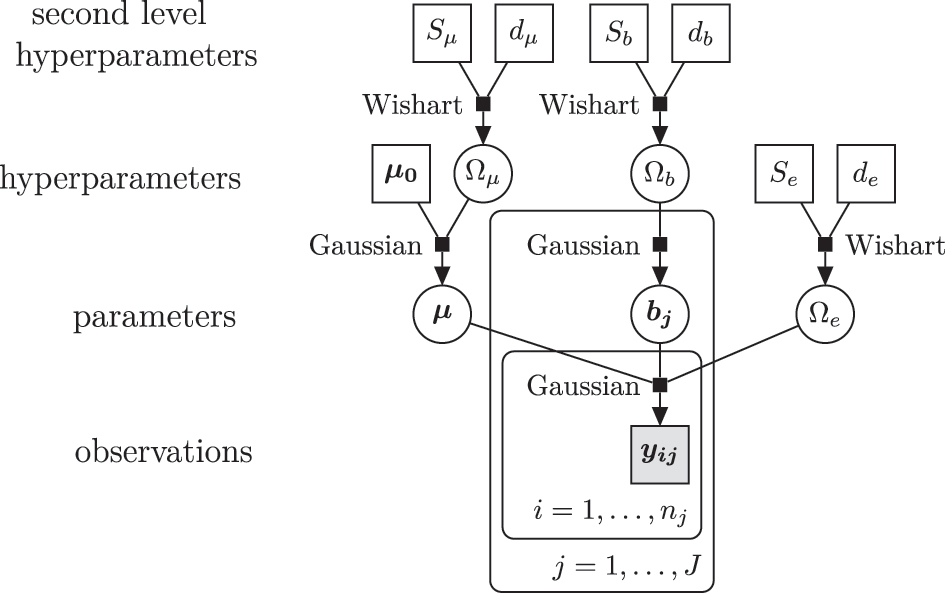
A graphical representation of the MBA with conjugate priors. The overall mean, μ , and the precision matrix, Ω _e , are assumed to be independent.

We approximate the posterior parameters by using Gibbs sampling [28], [29]. To apply the Gibbs sampler (see Algorithm 1), the full conditional posterior distributions for each of the unknown parameters of θ = μ , { μ j } j = 1 J , Ω e , Ω μ , Ω b are calculated as follows:

where in this section y is an n _j  × J × K data matrix and

3.1 One-class classification

One-class classification (OCC) algorithms are used in classification when only one class, called the “target” class, is fully known and the others are either absent or poorly sampled [30], [31], [32]. Doping detection constitutes a challenging topic in forensic toxicology, as standard binary classification procedures, such as the Naive Bayes classifier, are unsuitable due to the severe class imbalance. Consequently, doping detection can be framed as a one-class classification problem since measurements from doped athletes can be difficult to obtain, either due to the elaborated techniques that athletes use to avoid testing, or due to the undetectable use of banned substances.

For doping analysis, full information is provided on non-doped athletes who have been voluntarily tested, but limited knowledge is available for athletes who have received doping regimens. Thus, the samples from athletes with normal concentration values are treated as the “target” class. The focus is on studying whether there is evidence that new samples from athletes, whose doping status is unknown, are compatible with the known normal class of samples, or whether they show an abnormal pattern and should be considered as outliers. A classifier, that is a function which assigns each input data point to a class, accounting for other confounding factors such as sex, cannot be constructed with known standard rules in the case of imbalanced classes. In a machine learning context, the main purpose is to infer a classifier from a limited set of training data noting that, in addition to the complexity of unbalanced data, the classifier should also have the capability to deal with longitudinal data, their updating nature as well as potential confounders. We approach the one-class classification problem using a density estimation method applied to the multivariate Bayesian adaptive model introduced in Section 2.2. This model is trained exclusively on the majority class; i.e. normal values from non-doped athletes, as described in the following section.

3.2 Highest posterior predictive density

The Bayesian model specification contributes to hierarchically shift from the prior evidence about population parameters θ to the revised knowledge, expressed in the posterior density p( θ | y ), as new data become available. Using MCMC sampling methods, we can estimate the posterior density function and then approximate the K-variate predictive density function of a 1 × K new observable vector y _n+1 given the data y of dimensionality n _j′ × J′ × K, where J′ = J + 1. Therefore, the predictive density function is calculated as

which is formed by weighting the possible values of θ in the future observation f( y _n+1 | θ ) by how likely we believe they are to occur, p( θ | y ). Note that y consists of both data from the baseline longitudinal population, Y 0 n j × J × K , and all previous n normal recordings of the under study athlete J′, Y n × K = ( y 1 , … , y n ) ⊤ . It is important to highlight that the matrix Y ^n×K is dynamically updated for every sample classified as normal during the classification process. We can use the predictive distribution to provide a useful range of plausible concentration values for each new measurement added to the set of K markers and ratios of an athlete. This only applies to a single measurement at a time and not to the athlete’s entire profile. Specifically, y is the training set and consists of the samples from the “target” class; that is the concentration values from non-EAAS users, which are considered to be within the normal range. As we extend our method from univariate to multivariate, it is important to ensure a sufficient number of observations in the training set to overcome the curse of dimensionality and maintain the accuracy and performance of the model. The main task of the OCC algorithm is to define a classification boundary, such that it accepts as many samples as possible from the normal class, while it minimises the chance of accepting the outlier samples. Hence, the classification is performed by setting a threshold value, γ, on the approximated densities, in such a way that a target (normal) and a non-target (outlier/abnormal) region can be obtained ensuring a low predefined Type I error (false positive rate) α. Therefore, the 100(1 − α)% prediction interval for y _n+1 is the region of the form

where γ is the largest constant such that Pr( Y _n+1 ∈ C _α | y ) ≥ 1 − α [33], which serves as the criterion for classifying new recordings. A new test result y _n+1 is considered to be an outlier if, for at least one biomarker k, the corresponding observable y n + 1 ( k ) is not included in the 100(1 − α)% highest posterior density (HPD) intervals of its conditional probability distribution p k ( y n + 1 ( k ) | y 0 ( k ) , y 1 ( k ) , … , y n ( k ) ) , and normal otherwise.

Based on the decision rule in (9) the lower and upper limits of the HPD are obtained, which define the most credible normal boundaries of future EAAS concentrations or ratios. HPD intervals are robust to the shape of the posterior distribution and are not affected by outliers or skewness. These sample-specific boundaries can be used in detecting potential steroid misuse that may cause abnormally high or low concentration values of biomarkers or ratios, as well as in revealing urine sample replacement or the impact of other confounding factors. It is worth mentioning that there is the usual trade-off in choosing an appropriate α, since lower α values give wider intervals. High α values give narrower intervals implying that an extreme new measurement has a low probability of lying in the interval. Furthermore, note that testing the first measurement of a new athlete is based only on the population thresholds, since n = 0. Population thresholds are presented in Table B.6 of the Supplementary Material and were obtained by Van Renterghem et al. [16]. Further information about population thresholds was derived by Rauth [34] and Kicman et al. [35].

3.3 Continuity assumption

In this one-class classification process, we assume that the continuity assumption holds. This is a general assumption in pattern recognition, according to which points that are close to each other are more likely to share a label. For this purpose, when the model suggests an outlier, then this observation is automatically excluded from the set of recordings that are used to compute the HPD intervals for normal samples. If we do not discard the observations flagged up as outliers, we should expect to learn the noise, and any noise measurements which are considered as normal measurements have a significant impact on the personalised accepted limits. Hence, we cannot expect to infer a good classification in such a case.

4.1 Data summary

The proposed method was applied to athletes’ longitudinal steroid profile data extracted from their ABP. The datasets have been collected by following all the appropriate ethical approval procedures. Individual steroid profiles were analysed according to established methods including gas chromatography-mass spectrometry (GC-MS). Figure 2 represents a real GC-MS multiple reaction monitoring chromatogram produced by an unsuspicious urine sample. The longitudinal dataset includes six endogenous androgenic steroid concentrations and five concentration ratios proposed by WADA (i.e. T, E, A, Etio, A5, B5, T/E, A/T, A/Etio, A5/B5 and A5/E), which were repeatedly collected from each athlete in or out-of-competition.

Figure 2:

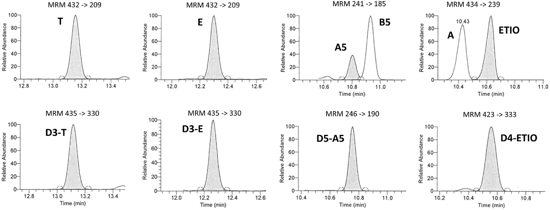
Extracted chromatograms obtained for an unsuspicious urine sample. Shown are the multiple reaction monitoring (MRM) ion transitions employed for the quantification of endogenous steroids (upper part) and their deuterated analogues (lower part).

A total of 1,433 normal urine samples were obtained from 100 athletes (50 males and 50 females), 2,504 samples were obtained from 100 athletes (50 males and 50 females) whose longitudinal steroid profiles contain values classified as atypical, and 462 samples from 29 athletes (15 males and 14 females) with at least one confirmed abnormal value in their steroid profile (Table 1), employing IRMS in line with WADA regulation [24]. Figure A.1 in the Supplementary Material shows that there is severe imbalance between normal (grey) and non-normal (black) samples with the former specifying the majority class. Specifically, out of 4,399 urine samples across all athletes, only 327 (7.43 %) were non-normal values (275 from athletes with atypical samples, and 52 from athletes with abnormal samples). Sample calibration was carried out prior to the analysis according to the estimated real limits of the applied methodology. Limit of detection (LOD) values and limit of quantification (LOQ) values within the steroid profiles of the athletes have been replaced by commonly accepted minimum cut-off values for all markers; i.e. all < LOQ and < LOD values in testosterone and epitestosterone were replaced by 1 ng/mL and 0.1 ng/mL respectively, while for < LOQ and < LOD values in the -diols were replaced by 5 ng/mL and 1 ng/mL, respectively.

Furthermore, single EAAS and ratio measurements of 164 healthy individuals have been provided as part of a separate cross-sectional study, representing a baseline population of which 91 were men and 73 women of age between 18 and 54 [19]. Figure A.2 in the Supplementary Material presents the scatter and density plots for men (black) and women (grey) for all available markers and ratios. The concentrations of markers seem to be slightly separable between men and women. However, this does not apply to the ratios, where the distributions of both sexes seem similar, except for the A/T ratio. The correlation between the various markers and ratios shows that plain markers are more highly correlated compared to the ratios (Figure A.2).

Tables B.2–B.5 in the Supplementary Material summarise the statistics (minimum, 1st quartile; Q1 and 3rd quartile; Q3, mean, median, maximum EAAS values and standard deviation) of the baseline cross-sectional population and the longitudinally-monitored athletes. The boxplots of the mean values of the available longitudinal metabolites and ratios are reported in Figure 3. When available, the WADA limits (lower and/or upper) are denoted by the solid lines based on Table B.6 of the Supplementary Material. Androsterone and Etiocholanolone share the same population thresholds among females and males. When population-specific information is unavailable for certain ratios, the Q3 values derived from the cross-sectional dataset are used as initial population thresholds for the respective ratios.

Figure 3:

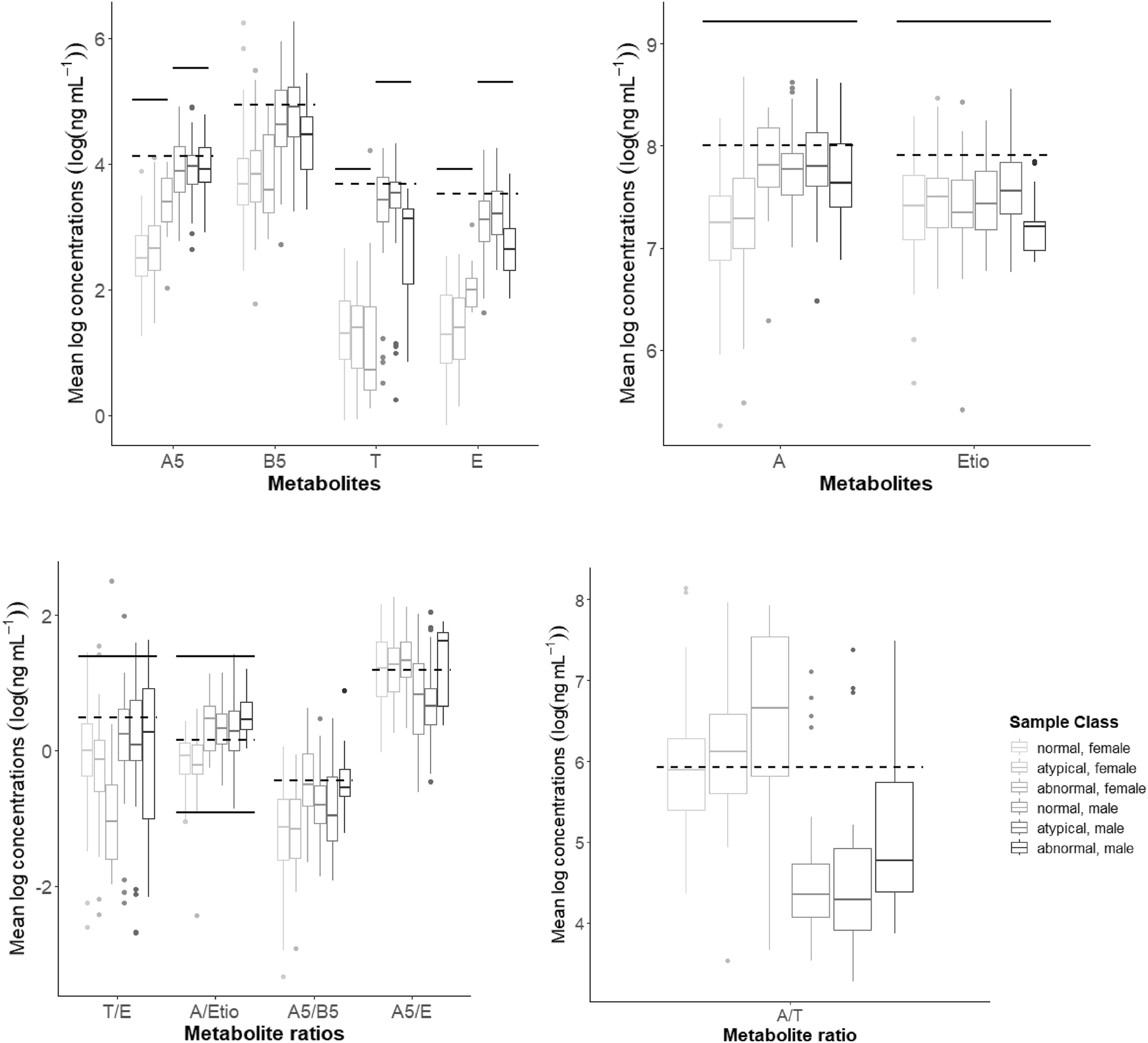
Boxplots for the mean logarithmic values of the metabolite concentrations (ng mL⁻¹) and their ratios from the longitudinal steroid profiles of the 229 athletes by sex and sample class. WADA log-limits are denoted by the solid lines. Dashed lines represent the mean log-concentrations of the metabolites obtained from the baseline cross-sectional population.

4.2 Estimation of highest posterior predictive density

4.2.1 Univariate HPD estimation

Here we fit the univariate Bayesian model to each athlete and each biomarker in the ABP separately. To implement the model, we initially specified the prior distributions for the model parameters as described in Equations (2) and (3). While the correlation between the empirical mean and precision of log-transformed concentration values across all markers was relatively weak, ranging from −0.33 to 0.32, we consider a prior dependency between the parameters μ and τ. We set the hyperparameters κ ₀ = 1, α ₀ = 10, and β ₀ = 1, while we control for possible confounding due to sex differences by setting μ 0 = y ̄ j s , that is the sample mean of the kth marker in its logarithmic scale for male subjects if s = 0, and for females if s = 1, obtained from the baseline cross-sectional dataset. After the burn-in period of 1,000 draws, 5,000 draws for each parameter were sampled from the known joint posterior distribution (Gaussian-Gamma). The out-of-sample predictive distribution of a new test result y _n+1 given the previous recordings y = (y ₁, y ₂, …, y _n ) is computed as

(10) p ( y n + 1 | y ) = ∬ p ( y n + 1 | μ , τ ) p ( μ , τ | y ) d μ d τ ≈ 1 T ∑ t = 1 T τ ( t ) 2 π 1 / 2 e − τ ( t ) 2 ( y n + 1 − μ ( t ) ) 2 ,

where n ≥ 0, and (μ ^(t), τ ^(t)) is the parameter pair of the tth draw obtained through the sampler with total number of iterations T = 5,000. In practice, the integration averaging is performed using an empirical average based on samples from the posterior distribution. At first, we simulate replicates of new data, y _n+1, from the posterior predictive distribution. Then we derive the 95 % HPD interval, using it as a criterion to classify a real data point as either a normal value or an outlier. Unlike the multivariate mixed-effects model in Section 2.2, this model cannot be applied to longitudinal data. Therefore, the available baseline longitudinal population cannot serve as a training set in this case. The univariate model constitutes an unsupervised learning approach, where the sample class is considered unknown. However, in our dataset, the true class for each of the 4,399 EAAS concentrations and ratios of 229 athletes is known, allowing us to estimate the predictive accuracy of the method.

In Figure 4, the A5 and T/E series of a doped athlete are depicted with the blue-solid lines. The red dotted lines are the 95 % HPD intervals of the predictive distribution, which serve as the posterior normal boundaries at each specific time point. Before observing any data, the upper limits are defined by WADA’s population thresholds, when they are available (see Table B.6 in the Supplementary Material). For marker B5, we used the maximum value obtained by the Caucasian population in Van Renterghem et al. [16], while for the remaining ratios (A5/B5, A5/E and A/T) we chose the Q3 values 4, 10 and 10,000, respectively, as reasonable starting thresholds derived from the cross-sectional dataset. The purple dashed lines indicate the usual Z-score upper limits as presented in Sottas et al. [17]. The gold diamonds symbolise the abnormal values in the athlete’s profile, which the model considers as suspicious values that need further investigation. For the T/E ratio in Figure 4(b), there are two additional green dashed-dotted lines that indicate the upper and lower limits of the T/E model with informative priors introduced by Sottas et al. [17]. For example, in Figure 4(a), there are two androsterone samples which are higher than the upper limits, and in Figure 4(b), Sottas’ model identifies four abnormal T/E tests, out of which three are in common with those suggested by the general univariate model.

Figure 4:

A series of 29 longitudinal values of (a) A5 and (b) T/E (blue solid-dotted line) obtained from a doped athlete; the upper and lower limits (red dotted lines) are the 95 % HPD intervals from the univariate Bayesian model; upper limits based on a usual Z-score (purple dashed line); abnormal values are marked with gold diamonds. For (b), upper and lower limits (green dashed-dotted lines) are the 95 % HPD interval from the T/E model of Sottas et al. [17], with its suggested abnormal values indicated by green stars.

Figure A.3(a)–(k) in the Supplementary Material displays the series of the six EAAS along with their five corresponding ratios for the same athlete. Given that the 21st, 22nd and 23rd sample tests of that athlete are confirmed as abnormal, only E, T/E and A5/E were sensitive enough to detect these anomalies within the athlete’s steroid profile. Note that if the model suggests a sample as an outlier, we automatically exclude it from the set of recordings which are used to compute the HPD intervals, because it might have an impact on the validity of the following personalised normal limits.

4.3 Classification performance

In forensic toxicology, high specificity is important, thus a very low false positive rate is required in order to prevent the accusation of an innocent athlete. However, classification accuracy values and measures regarding the majority class such as the overall accuracy, tend to be pretty high because they are computed under the assumption of balanced class distributions. Consequently, we use appropriate metrics for evaluating the classification performance of the models which can deal with the imbalance of the dataset, such as the F1 score and G-mean (Geometric mean) defined as

and

Tables 2 and 3 present the classification performance of the univariate model and the MBA model in comparison with the univariate T/E model proposed by Sottas et al. [17], the univariate Euclidean distance (ED) score model of De Figueiredo et al. [26] and a generalised linear mixed-effects model (GLMM) using a false positive rate α = 0.05. The GLMM model is implemented via the glmer() function from the lme4 package in R [37] to fit a mixed effects logistic regression model with a binomial distribution for the response variable “Class _ij ”, which is a binary variable that represents the class of each observation i of athlete j including the biomarkers and/or ratios as individual level continuous predictors, and a random intercept by athlete ID. The problem of unreliable overall accuracy in binary class classification with imbalanced data through the GLMM has been alleviated by the application of oversampling, as evidenced by the now equivalent values of balanced accuracy and overall accuracy (see Table 3).

The classification using the univariate models suggest the T/E, A/ETIO and A5/E ratios as the most sensitive variables for detecting anomalies in the steroidal profile with higher F1 scores ( F 1 T/E a = 0.19 , F1_A/ETIO = 0.24 and F1_A5/E = 0.23). Regarding the T/E models, the one employing informative priors demonstrates slightly better predictive performance in contrast to the model using semi-informative conjugate priors, as indicated by the improved metrics F 1 T/E b = 0.20 , sensitivity T/E b = 0.32 and balanced accuracy T/E b = 0.59 . In Figure 5, we have also presented the ROC (Receiver Operating Characteristic) curves and the Precision-Recall curves to measure the accuracy of the classification predictions in the various models. According to the ROC curves, the model for the A5/E ratio showed superiority compared to the other univariate models in Figure 5(a), while the model for A/ETIO ratio showed superiority in the Precision-Recall plot. However, the superior performance of the A/ETIO ratio was unexpected based on the current literature, which is an aspect that warrants further investigation. The curve using the model of Sottas et al. [17] for T/E is higher in Figure 5(b), which verifies its higher predictive performance.

Figure 5:

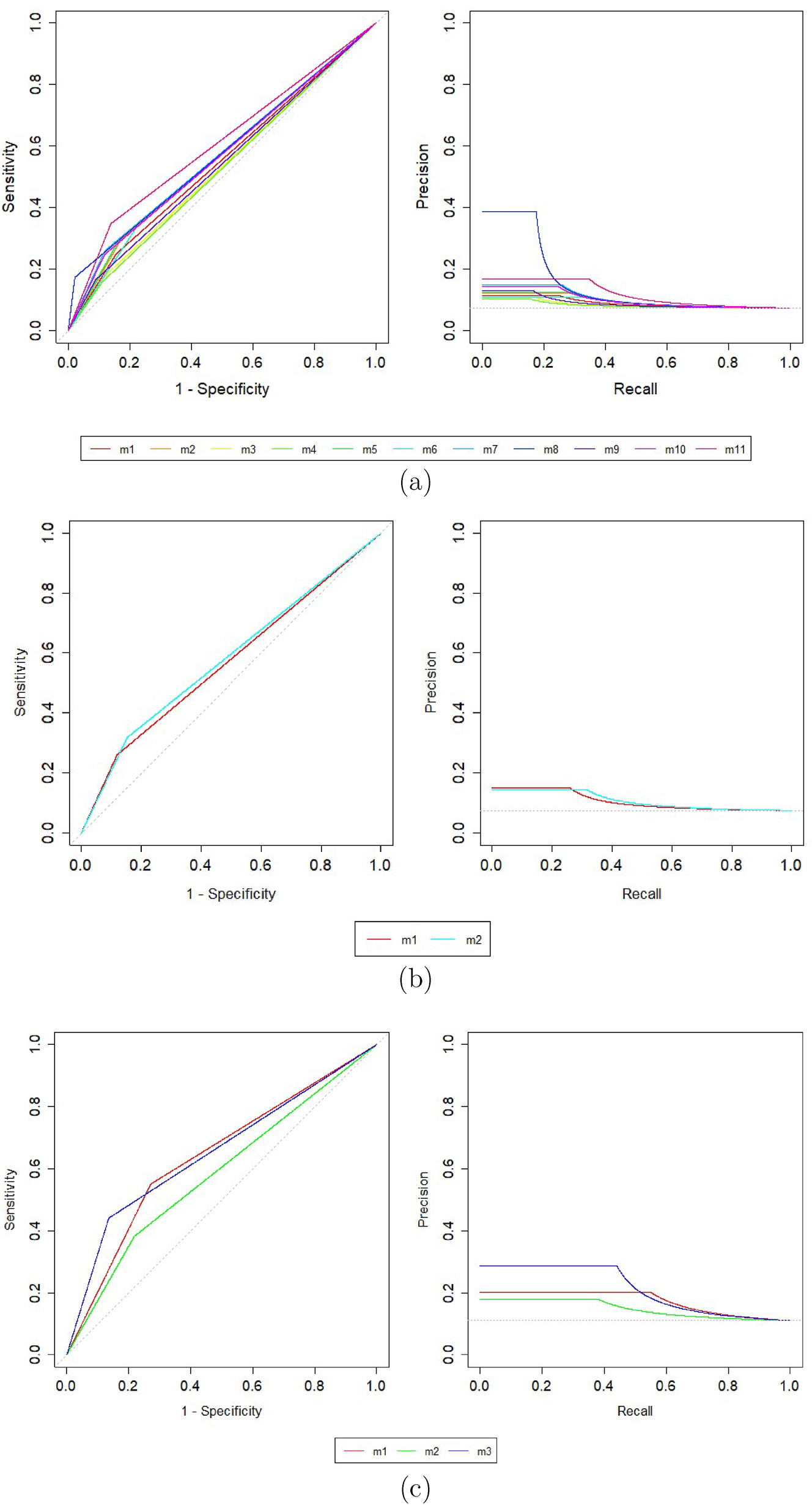
ROC curves obtained from (a) the univariate models (m1: A5, m2: B5, m3: A, m4: ETIO, m5: T, m6: E, m7: T/E, m8: A/ETIO, m9: A/T, m10: A5/B5, m11: A5/E), (b) m1: T/E model versus m2: Sottas’ model for T/E, and (c) the multivariate models (m1: all EAAS markers and ratios, m2: EAAS only, m3: ratios only) applied to the longitudinal test set.

The proposed multivariate Bayesian adaptive (MBA) model has been applied to: (a) EAAS markers only; (b) ratios only; and (c) all EAAS markers and ratios. Evaluating the F1 scores of MBA in Table 2, it appears that MBA achieves an improved classification performance across all models. Further, we observe that the univariate ED score model exhibits considerably higher sensitivity and lower specificity values, indicating a tendency to classify normal values as abnormal. Conversely, in Table 3, the GLMM performance is characterised by significantly higher specificity and lower sensitivity, suggesting a tendency to classify abnormal values as normal. Therefore, their F1 score values are biased towards either very high or very low sensitivity. To address this, we employ the G-mean metric to compare all models, which is the harmonic mean of sensitivity and specificity, as defined in Equation (13). The highest G-mean values are consistently achieved by the multivariate Bayesian adaptive models, which overall outperform univariate (e.g. A5, B5, A) and multivariate models (univariate ED score and GLMM).

As shown in Table 2, between the applications of the MBA model the G-mean and F1 metrics exhibit consistently higher values when compared to their counterparts in the univariate models. Comparing further between the performance of the MBAs, the five available ratios were found to be the most powerful set of variables with the highest metric values F 1 MBA ratios = 0.35 , precision MBA ratios = 0.29 , specificity MBA ratios = 0.87 , balanced accuracy MBA ratios = 0.65 and highest overall accuracy  MBA ratios = 0.82 . While the G-mean value for the model applied to the five ratios ( G − mean MBA ratios = 0.62 ) , is slightly lower that of the corresponding model applied to the six markers and five ratios together ( G − mean MBA all = 0.63 ) , it is important to note that the model focusing on the ratios remains equally powerful despite utilising less information. Similar conclusions about the superiority of the multivariate model, assessed through the use of ratios, can be derived from an examination of the plots in Figure 5(c). Here, the blue lines point to a better relationship between sensitivity and 1-specificity, as well as between precision and recall. In Figure 6, all classification metrics are plotted for the applied models. Once more, the conclusion is clear that the multivariate Bayesian adaptive model (MBA) applied solely to the ratios, consistently delivers the best overall classification performance ( F 1 MBA ratios = 0.35 and G- mean MBA ratios = 0.62 ) compared to the univariate models, the univariate ED score models and the GLMMs.

Figure 6:

Classification metrics per component; i.e. markers and ratios separately, only EAAS, only ratios, all EAAS markers and ratios. T/E₁ corresponds to the T/E model from Section 2.1, while T/E₂ corresponds to the T/E model by Sottas et al. [17]. Subscripts “pre”, “post”, denote pre-oversampling and post-oversampling, respectively.

References

1. Kanayama, G, Pope Jr, HG. History and epidemiology of anabolic androgens in athletes and non-athletes. Mol Cell Endocrinol 2018;464:4–13. https://doi.org/10.1016/j.mce.2017.02.039.Search in Google Scholar PubMed
2. World Anti-Doping Agency. 2021 Anti-doping testing figures [Online]. https://www.wada-ama.org/sites/default/files/2023-01/2021_anti-doping_testing_figures_en.pdf [Accessed 19 Feb 2024].Search in Google Scholar
3. Sottas, PE, Saugy, M, Saudan, C. Endogenous steroid profiling in the athlete biological passport. Endocrinol Metabol Clin 2010;39:59–73. https://doi.org/10.1016/j.ecl.2009.11.003.Search in Google Scholar PubMed
4. World Anti-Doping Agency. Technical document – TD2021EAAS [Online]. https://www.wada-ama.org/sites/default/files/2022-01/td2021eaas_final_eng_v_2.0.pdf [Accessed 19 Feb 2024].Search in Google Scholar
5. Sottas, PE, Robinson, N, Rabin, O, Saugy, M. The athlete biological passport. Clin Chem 2011;57:969–76. https://doi.org/10.1373/clinchem.2011.162271.Search in Google Scholar PubMed
6. Vernec, AR. The athlete biological passport: an integral element of innovative strategies in antidoping. Br J Sports Med 2014;48:817–19. https://doi.org/10.1136/bjsports-2014-093560.Search in Google Scholar PubMed
7. World Anti-Doping Agency. WADA technical document – TD2021APMU [Online]. https://www.wada-ama.org/sites/default/files/resources/files/td2021apmu_final_eng_0.pdf [Accessed 19 Feb 2024].Search in Google Scholar
8. Kuuranne, T, Saugy, M, Baume, N. Confounding factors and genetic polymorphism in the evaluation of individual steroid profiling. Br J Sports Med 2014;48:848–55. https://doi.org/10.1136/bjsports-2014-093510.Search in Google Scholar PubMed PubMed Central
9. Piper, T, Geyer, H, Haenelt, N, Huelsemann, F, Schaenzer, W, Thevis, M. Current insights into the steroidal module of the athlete biological passport. Int J Sports Med 2021;42:863–78. https://doi.org/10.1055/a-1481-8683.Search in Google Scholar PubMed PubMed Central
10. Mareck, U, Geyer, H, Opfermann, G, Thevis, M, Schänzer, W. Factors influencing the steroid profile in doping control analysis. J Mass Spectrom 2008;43:877–91. https://doi.org/10.1002/jms.1457.Search in Google Scholar PubMed
11. Harris, EK. Effects of intra-and interindividual variation on the appropriate use of normal ranges. Clin Chem 1974;20:1535–42. https://doi.org/10.1093/clinchem/20.12.1535.Search in Google Scholar
12. Brooks, RV, Jeremiah, G, Webb, WA, Wheeler, M. Detection of anabolic steroid administration to athletes. J Steroid Biochem 1979;11:913–17. https://doi.org/10.1016/b978-0-08-023796-1.50129-8.Search in Google Scholar
13. Donike, M, Barwald, K, Klostermann, KR, Schanzer, W, Zimmermann, J. Nachweis von exogenem testosteron [detection of exogenous testosterone]. Sport: Leistung und Gesundheit 1983;293–8.Search in Google Scholar
14. Sottas, PE, Robinson, N, Giraud, S, Taroni, F, Kamber, M, Mangin, P, et al.. Statistical classification of abnormal blood profiles in athletes. Int J Biostat 2006;2. https://doi.org/10.2202/1557-4679.1011.Search in Google Scholar
15. Sottas, P-E, Saudan, C, Schweizer, C, Baume, N, Mangin, P, Saugy, M. From population-to subject-based limits of T/E ratio to detect testosterone abuse in elite sports. Forensic Sci Int 2008;174:166–72. https://doi.org/10.1016/j.forsciint.2007.04.001.Search in Google Scholar PubMed
16. Van Renterghem, P, Van Eenoo, P, Geyer, H, Schänzer, W, Delbeke, FT. Reference ranges for urinary concentrations and ratios of endogenous steroids, which can be used as markers for steroid misuse, in a Caucasian population of athletes. Steroids 2010;75:154–63. https://doi.org/10.1016/j.steroids.2009.11.008.Search in Google Scholar PubMed
17. Sottas, P-E, Baume, N, Saudan, C, Schweizer, C, Kamber, M, Saugy, M. Bayesian detection of abnormal values in longitudinal biomarkers with an application to T/E ratio. Biostatistics 2007;8:285–96. https://doi.org/10.1093/biostatistics/kxl009.Search in Google Scholar PubMed
18. Brown, PJ, Kenward, MG, Bassett, EE. Bayesian discrimination with longitudinal data. Biostatistics 2001;2:417–32. https://doi.org/10.1093/biostatistics/2.4.417.Search in Google Scholar PubMed
19. Alladio, E, Caruso, R, Gerace, E, Amante, E, Salomone, A, Vincenti, M. Application of multivariate statistics to the steroidal module of the athlete biological passport: a proof of concept study. Anal Chim Acta 2016;922:19–29. https://doi.org/10.1016/j.aca.2016.03.051.Search in Google Scholar PubMed
20. Amante, E, Pruner, S, Alladio, E, Salomone, A, Vincenti, M, Bro, R. Multivariate interpretation of the urinary steroid profile and training-induced modifications. The case study of a marathon runner. Drug Test Anal 2019;11:1556–65. https://doi.org/10.1002/dta.2676.Search in Google Scholar PubMed
21. Wang, M, Li, Z, Lee, EY, Lewis, MM, Zhang, L, Sterling, NW, et al.. Predicting the multi-domain progression of Parkinson’s disease: a Bayesian multivariate generalized linear mixed-effect model. BMC Med Res Methodol 2017;17:1–10. https://doi.org/10.1186/s12874-017-0415-4.Search in Google Scholar PubMed PubMed Central
22. Xia, YM, Tang, NS. Bayesian analysis for mixture of latent variable hidden Markov models with multivariate longitudinal data. Comput Stat Data Anal 2019;132:190–211. https://doi.org/10.1016/j.csda.2018.08.004.Search in Google Scholar
23. Shamshoian, J, Şentürk, D, Jeste, S, Telesca, D. Bayesian analysis of longitudinal and multidimensional functional data. Biostatistics 2022;23:558–73. https://doi.org/10.1093/biostatistics/kxaa041.Search in Google Scholar PubMed PubMed Central
24. World Anti-Doping Agency. WADA technical document – TD2021IRMS [Online]. https://www.wada-ama.org/sites/default/files/resources/files/td2021irms_final_eng_0.pdf [Accessed 19 Feb 2024].Search in Google Scholar
25. R Core Team. The R project for statistical computing [Online]https://www.r-project.org/ [Accessed 20 Oct 2023].Search in Google Scholar
26. De Figueiredo, M, Saugy, J, Saugy, M, Faiss, R, Salamin, O, Nicoli, R, et al.. A new multimodal paradigm for biomarkers longitudinal monitoring: a clinical application to women steroid profiles in urine and blood. Anal Chim Acta 2023;1267:341389. https://doi.org/10.1016/j.aca.2023.341389.Search in Google Scholar PubMed
27. DeGroot, MH. Optimal statistical decisions. Hoboken, New Jersey, United States: John Wiley & Sons; 2005, 82.Search in Google Scholar
28. Casella, G, George, EI. Explaining the Gibbs sampler. Am Statistician 1992;46:167–74. https://doi.org/10.1080/00031305.1992.10475878.Search in Google Scholar
29. Gelman, A, Carlin, JB, Stern, HS, Dunson, DB, Vehtari, A, Rubin, DB. Bayesian data analysis. Boca Raton, Florida, United States: CRC Press; 2013.10.1201/b16018Search in Google Scholar
30. Minter, T. Single-class classification. In: LARS symposia; 1975:54 p.10.5179/benthos1970.1975.54Search in Google Scholar
31. Bishop, CM. Novelty detection and neural network validation. IEE Proc Vis Image Signal Process 1994;141:217–22. https://doi.org/10.1049/ip-vis:19941330.10.1049/ip-vis:19941330Search in Google Scholar
32. Khan, SS, Madden, MG. One-class classification: taxonomy of study and review of techniques. Knowl Eng Rev 2014;29:345–74. https://doi.org/10.1017/s026988891300043x.Search in Google Scholar
33. Hyndman, RJ. Computing and graphing highest density regions. Am Statistician 1996;50:120–6. https://doi.org/10.1080/00031305.1996.10474359.Search in Google Scholar
34. Rauth, S. Referenzbereiche von urinären Steroidkonzentrationen und Steroidquotienten: ein Beitrag zur Interpretation des Steroidprofils in der Routinedopinganalytik [Ph.D. thesis]. Deutsche Sporthochschule Köln; 1994.Search in Google Scholar
35. Kicman, AT, Coutts, SB, Walker, CJ, Cowan, DA. Proposed confirmatory procedure for detecting 5 alpha-dihydrotestosterone doping in male athletes. Clin Chem 1995;41:1617–27. https://doi.org/10.1093/clinchem/41.11.1617.Search in Google Scholar
36. Eleftheriou, D. Bayesian hierarchical modelling for biomarkers with applications to doping detection and prostate cancer prediction [Ph.D. thesis]. University of Glasgow; 2022.Search in Google Scholar
37. Bates, D, Mächler, M, Bolker, B, Walker, S. Fitting linear mixed-effects models using lme4. J Stat Software 2015;67:1–48. https://doi.org/10.18637/jss.v067.i01.Search in Google Scholar
38. Kotsiantis, S, Kanellopoulos, D, Pintelas, P. Handling imbalanced datasets: a review. GESTS Int Trans Comput Sci Eng 2006;30:25–36.Search in Google Scholar
39. Schapire, RE. Empirical inference. Berlin, Germany: Springer; 2013:37–52 pp.10.1007/978-3-642-41136-6_5Search in Google Scholar
40. Wilkes, EH, Rumsby, G, Woodward, GM. Using machine learning to aid the interpretation of urine steroid profiles. Clin Chem 2018;64:1586–95. https://doi.org/10.1373/clinchem.2018.292201.Search in Google Scholar PubMed
Supplementary Material
This article contains supplementary material (https://doi.org/10.1515/ijb-2024-0019).
© 2025 the author(s), published by De Gruyter, Berlin/Boston
This work is licensed under the Creative Commons Attribution 4.0 International License.
Articles in the same Issue
- Frontmatter
- Research Articles
- Prognostic adjustment with efficient estimators to unbiasedly leverage historical data in randomized trials
- Homogeneity test and sample size of response rates for AC 1 in a stratified evaluation design
- A review of survival stacking: a method to cast survival regression analysis as a classification problem
- DsubCox: a fast subsampling algorithm for Cox model with distributed and massive survival data
- A hybrid hazard-based model using two-piece distributions
- Regression analysis of clustered current status data with informative cluster size under a transformed survival model
- Bayesian covariance regression in functional data analysis with applications to functional brain imaging
- Risk estimation and boundary detection in Bayesian disease mapping
- An improved estimator of the logarithmic odds ratio for small sample sizes using a Bayesian approach
- Short Communication