Regression analysis of interval-censored failure time data under semiparametric transformation models with missing covariates

1 Introduction

This paper discusses regression analysis of interval-censored failure time data arising from semiparametric transformation models in the presence of missing at random covariates. By interval-censored data, we usually mean that the failure time of interest is observed or known only to belong to an interval instead of being known exactly, and they can often occur in various fields such as periodic follow-up studies and clinical trials [1], 2]. Also they include right-censored data as a specific case [3]. For regression analysis of failure time data, semiparametric transformation models have become more popular due to their flexibility in capturing diverse covariate effects [4], [5], [6], [7], [8]. In particular, they include the proportional hazards and odds models as special instances.

One example of interval-censored data that motivated this study is given by the Alzheimer’s Disease Neuroimaging Initiative (ADNI). This longitudinal multi-center follow-up study, launched in 2004, aims to identify the biomarkers for early detection and monitoring of Alzheimer’s Disease (AD). Among others, one variable of interest is the onset of AD conversion [9], 10], and due to the periodic follow-up nature, only interval-censored are available for the occurrence time of AD conversion. Furthermore, there exist missing values on some covariates or biomarkers. More details about the study will be given below.

Missing covariates occur in almost every field and it is well-known that their impact on statistical analyses and the results can be substantial if not properly taken into account [11]. In particular, the missing mechanism plays an important role and two types of commonly studied mechanisms are missing completely at random (MCAR) and missing at random (MAR). Correspondingly two commonly used analysis approaches are the complete-case analysis and the inverse probability weighting (IPW). The former bases the analysis solely on complete cases or excludes the observations with missing values, and it is easy to see that although easily implementable, it may be less efficient and produce biased estimates under some specific MAR schemes [12]. The IPW approach introduces weights to the complete-case analysis aiming to mitigate potential estimation biases associated with the former by modeling the missing mechanism instead of the distribution of partially observed variables [13]. Thus its validity is highly contingent on an accurate model of the missing mechanism. Also as the former, it may be inefficient.

Several methods have been developed for regression analysis of interval-censored failure time data with missing covariates. For example, Wen and Lin [14] considered the problem for current status data, a special case of interval-censored data, meaning that the censoring interval includes either zero or infinity or the failure time of interest is either left- or right-censored. Li et al. [15] and Zhou et al. [16] also investigated the problem for the cases where the failure time follows the additive hazards model and the proportional hazards model, respectively. In particular, the latter relies on high-dimensional integrals, resulting in a complex algorithm that may be challenging to generalize to other hazard models. Nevertheless, there does not seem to exist an established procedure for estimating the semiparametric transformation model based on interval-censored data with missing covariates.

The multiple imputation approach has been commonly used for the analysis of missing data. However, the conventional multiple imputation procedures face challenges when dealing with interval-censored outcomes and can result in substantial biases as pointed out by Zhou et al. [16]. In this paper, we introduce a novel multiple imputation procedure tailored for regression analysis of interval-censored data arising from the semiparametric transformation model under the MAR assumption. The key innovation involves leveraging two predictive scores for each subject and subsequently forming a neighborhood set. This set comprises fully observed data points with similar predictive scores, serving as the imputation set for missing observations. The idea was initially proposed by Long et al. [17] for complete data and later extended to right-censored data under the Cox model by Hsu and Yu [12]. In the proposed method, we use Turnbull’s self-consistency estimator [18] for the predictive scores to integrate survival outcome information, and the sieve maximum likelihood estimation procedure is employed after the imputation. It is intuitive and can be readily implemented using the standard software.

The remainder of the paper is organized as follows. In Section 2, we will first introduce some notation and assumptions that will be used throughout the paper and then discuss the structure of the observed data and the missing mechanism. Section 3 will briefly review the existing estimation procedure for the situation of no missing covariates and the two naive methods mentioned above, and the proposed multiple imputation approach will be presented in Section 4. A simulation study is conducted to assess the performance of the proposed method in Section 5 and suggests that it works well in practical situations. In Section 6, we apply the proposed approach to the ADNI study discussed above, and Section 7 concludes with some discussion and concluding remarks.

2 Notation and assumptions

Consider a failure time study that involves n independent subjects. For subject i, let T _i denote the failure time of interest, and suppose that there exist two sets of covariates denoted by Z i ∈ R p and X i ∈ R q , where X _i contains missing values, and Z _i encompasses all fully observed covariates. In the following, we will assume that given the covariate X i T , Z i T T , T _i follows the class of semiparametric transformation models with the cumulative hazard function given by

In the above, α and β denote q × 1 and p × 1 vector of regression coefficients, respectively. G(⋅) is a pre-specified, strictly increasing transformation link function, and Λ₀(t) denotes an unknown increasing baseline cumulative hazard function.

As mentioned above, the model above offers significant flexibility and includes various widely used models as special cases. For instance, it yields the proportional hazards model and the proportional odds model with G(x) = x and G(x) = log(1 + x), respectively. Also two commonly used classes of transformation functions are the Box-Cox transformation and logarithmic transformations, represented by G(x) = [(1 + x) ^ρ − 1]/ρ and G(x) = log(1 + ρx)/ρ, respectively, with ρ ≥ 0. One can easily show that under the model above, the survival function of T _i takes the form S ( t ∣ X i , Z i ) = exp − G Λ 0 ( t ) exp X i T α + Z i T β .

For the observed data, suppose that each subject is observed at a sequence of observation times 0 = V 0 , i < V 1 , i < … < V J i , i , where J _i denotes the number of the observation times. Let V i = ( V 0 , i , V 1 , i , … , V J i , i ) and define Δ _i = 1 if subject i is right-censored or if T i > V J i , i and zero otherwise. Furthermore, let (L _i , R _i ] denote the smallest interval to which T _i is observed to belong and define the vector of missing indicators χ i = ( χ i , 1 , … , χ i , q ) T with χ _i,j = 1 if X _i,j is fully observed and χ _i,j = 0 if X _i,j is missing, j = 1, …, q. Also we define χ ̃ i [ 1 ] = ∏ j = 1 q χ i , j , denoting whether the individual has no missing values. The observed data then take the form O = { O i } i = 1 n , where O _i = {L _i , R _i , Δ _i , Z _i , χ _i , χ _i × X _i }. In this context, when χ _i,j = 0, we have X i j = N A . Additionally, we define that 0 × N A = N A .

In the following, for simplicity, we will assume that the missing mechanism is MAR [19] or we have

and

In other words, the probability that data are missing depends only on the observed parts but not on the missing parts. The MAR reduces to MCAR if the probability above is constant [20], 21]. Note that here for mathematical simplicity, we assume that the missing mechanism relies solely on the covariates that have no missing components, not the covariates that contain some missing values.

3 Naive estimation procedures

In this section, we will first briefly review the estimation approach when there were no missing covariates and then introduce two aforementioned naive estimation procedures for the missing covariates. Note that under the assumptions above, if we have the full data without missing, the benchmark log-likelihood function has the form

For the situation, several methods have been given in the literature to estimate the unknown parameter θ = ( α , β , Λ₀) [1]. In particular, one can employ the sieve maximum likelihood approach that approximates the unknown function Λ₀(t) using Bernstein polynomials before the maximization [8], 22].

More specifically, define the parameter space Θ = { θ = ( η , Λ 0 ) ∈ B ⊗ M } , where B = { η = ( α T , β T ) T ∈ R p + q : | | η | | ≤ M } with M being a positive constant and M is the collection of all bounded and continuous nondecreasing, nonnegative functions over interval [t _l , t _u ] with 0 ≤ t _l < t _u < ∞. Also define the sieve space Θ n = { θ n = ( η n , Λ 0 n ) ∈ B ⊗ M n } , where η n = α n T , β n T T , and

In the above, M _n ensures that the Λ_0n is bounded and

with the degree m = o(n ^ν ) for some ν ∈ (0, 1). The sieve maximum likelihood estimator of θ is then defined as the value of θ that maximizes the log-likelihood function ℓ ( θ ∣O) over Θ _n . By approximating the nonparametric function using Bernstein polynomials, it transforms the semiparametric problem into a parametric one, making it much easier to handle and manipulate.

Now suppose that there exist missing covariates. As mentioned above, one commonly used approach is the complete-case analysis that bases the estimation only on the samples with complete data and maximizes the observed log-likelihood function

with the use of the sieve approach mentioned earlier. As described above, one advantage of this method is its ease of implementation. However, if the proportion of missing data is large, it can result in significant information loss, reduced efficiency and substantial bias as will be demonstrated in the simulation study below.

As discussed above, instead of the complete-case analysis, one may employ the inverse probability weighted (IPW) approach, which is essentially a two-step approach. It first assumes a model for the probability of being observed as π i ( γ ) = P ( χ ̃ i [ 1 ] = 1 ∣ L i , R i , Δ i , Z i ; γ ) , where γ denotes a vector of unknown parameters. For simplicity, we assume that π _i ( γ ) follows a parametric or semiparametric model and the parameter γ can be consistently estimated [15], 16]. Among others, one commonly used model is the logistic regression model given by π i ( γ ) = exp W i T γ / 1 + exp W i T γ , where W _i is a vector that contains some or all components of (L _i , R _i , Δ _i , Z _i ). Let γ ̂ denote the estimator of γ . The IPW method then maximizes the weighted log-likelihood function

It is easy to see that this approach can make use of the observed information from both complete and incomplete cases and thus is expected to yield more efficient estimators than the complete-case analysis [13]. On the other hand, one drawback is that one needs the correctly specified missing probability to obtain a stable and valid IPW estimator. Furthermore, even with the correctly specified model, the procedure may encounter challenges if some values of π i ( γ ̂ ) are close to 0.

4 Multiple imputation estimation

Now we present the proposed multiple imputation estimation procedure. As mentioned previously, the basic idea behind it is to construct two predictive scores for each individual and then build a neighborhood set that comprises fully observed individuals for each individual with missing information. Subsequently, we generate a pseudo-observation value for the individual with a missing covariate from its neighborhood set for the imputation. After imputing all of the missing values, we treat the imputed dataset as the observed data to carry out the estimation based on the log-likelihood function given in (2) as described in the previous section. In the following, for simplicity, we will focus on the situation of q = 1. The proposed algorithm can be easily generalized to the case where q > 1 and more details on it will be given in Appendix A.

For each individual, we define two predictive scores, ζ ̃ and ζ ̄ , serving as indices for the individual’s values of X and the chance of being missing, respectively. To accomplish this, we propose two working models by generalized linear regression models for the values of X and its missing indicator χ to obtain the predictive scores. For the working models, a straightforward approach is to directly fit models for the values of X and its missing indicator χ using fully observed covariates Z. However, this may not be sufficient, even under right-censored data. White and Royston [23] pointed out that in the simple case of right-censored data from the proportional hazards model with binary variables X and Z, the conditional distribution for X follows a binomial distribution with logit{P(X = 1∣T, Δ, Z)} = a ₀ + a ₁Δ + a ₂ Λ₀(t) + a ₃ Z + a ₄ Z Λ₀(t). This implies that, even under right censoring, one should not only consider fully observed covariates, as the approximate conditional distribution depends on the cumulative baseline hazard, censoring indicator, and the fully observed covariate – all of which need to be included in the working models for predicting the values of X. Hsu and Yu [12] suggested incorporating the observed failure time and the baseline cumulative hazard into the predictive scores under right censoring. However, given our interval censoring setting where T can not be accurately observed and the missing scheme of X can also be dependent on the interval-censored outcomes, a more comprehensive approach is necessary.

A reasonable idea is to incorporate information from the interval-censored survival outcome, cumulative baseline hazard, missing indicator, and fully observed covariates into the working models. To achieve this, we first obtain the nonparametric survival function estimator S ̃ 0 ( t ) by using Turnbull’s self-consistency algorithm [18]. This yields estimators S ̃ 0 ( L ) and S ̃ 0 ( R ) , which, notably, involve information from the cumulative baseline hazard and the interval-censored survival outcome. Consequently, we use W ̃ = { S ̃ 0 ( L ) , S ̃ 0 ( R ) , Δ , Z } as the arguments for the working models. Specifically, we fit a linear/generalized linear regression model (Model H ₁(⋅)) with W ̃ as the covariate to the complete cases to obtain the predictive score for values of X, denoted as ζ ̃ . This score summarizes the relationship between X and W ̃ . Simultaneously, we fit a logistic regression model (Model H ₂(⋅)) with W ̃ as the covariate to the missing indicator χ, obtaining the predictive score for missingness, denoted as ζ ̄ . This score summarizes the relationship between χ and W ̃ .

Given the predictive score ζ i = ( ζ ̃ i , ζ ̄ i ) , we define the distance between two subjects, say, subjects k and j, as

Note that in (5), the first part with weight ω ₁ governs the observed distribution by modeling the relationships between X and W ̃ , highlighting the importance of predictive scores for missing values. In contrast, the second part governs the missing data mechanism by modeling the relationships between χ and W ̃ , emphasizing the significance of predictive scores for being missing. Given that our primary objective is to impute the values of X, a weight ω ₁ relatively close to 1 such as 0.8, is typically sufficient. One can also set ω ₁ to 1 for the MCAR scenario, effectively ignoring the second part. However, including it can enhance the coverage of information in the distance metric and improve the stability of neighbor identification based on this distance. More details are provided below. We further define the neighborhood set by selecting small distances (5) based on two predictive scores and utilize it as the imputation set.

To ensure a proper imputation scheme that fully encompasses the uncertainty in the imputed values, we employ the bootstrap strategy to approximate the uncertainty in parameter estimates [24], [25], [26]. The detailed multiple imputation procedures are outlined as follows.

[Step 1] Bootstrap Sampling.

• Obtain a bootstrap sample B ( s ) = B 1 ( s ) , … , B n ( s ) from the original dataset O. The complete cases within this bootstrap sample are denoted as B obs ( s ) = B [ 1 ] ( s ) , … , B [ n ( s ) ] ( s ) .

[Step 2] Self-Consistency Algorithm.

1. Apply Turnbull’s self-consistency algorithm to B ^(s) to obtain W ̃ ( s ) .

2. Perform the same procedure on O to obtain W ̃ .

[Step 3] Model Fitting.

1. Fit models H ₁(⋅) and H ₂(⋅) using B obs ( s ) and B ^(s), respectively. This will yield the estimates H ̂ 1 ( s ) ( ⋅ ) and H ̂ 2 ( s ) ( ⋅ ) .

2. Calculate the initial predictive scores ζ ̃ 0 ( s ) for each individual in B obs ( s ) and ζ ̄ 0 ( s ) for each individual in B ^(s).

3. Standardize the scores by subtracting the sample mean and dividing by the standard deviation, resulting in standardized scores ( ζ ̃ ( s ) , ζ ̄ ( s ) ) for the individual in B obs ( s ) .

[Step 4] Impute Missing Values for X.

1. For each missing value X _k associated with individual O _k in O, apply the estimated working models H ̂ 1 ( s ) ( ⋅ ) and H ̂ 2 ( s ) ( ⋅ ) to compute its initial predictive score.

2. Standardize these scores by subtracting the sample mean of the bootstrap predictive scores and dividing by the standard deviation of the bootstrap predictive scores, resulting in standardized scores ( ζ ̃ k , ζ ̄ k ) .

3. Use the pre-specified ω ₁ to calculate the distance D _k = {D(k, [1]), …, D(k, [n ^(s)])} between O _k and the individuals in B obs ( s ) as

   D ( k , [ j ] ) = ω 1 ζ ̃ k − ζ ̃ [ j ] ( s ) 2 + ( 1 − ω 1 ) ζ ̄ s − ζ ̄ [ j ] ( s ) 2 1 / 2 , j = 1 , … , n ( s ) .

4. Define a neighborhood set consisting of nearest neighbor (NN) subjects from B ^(s) by sorting distances in ascending order. Then, randomly draw a pseudo observation value for X _k from the observed values of X ^(s) within this neighborhood set.

[Step 5] Final Estimation.

After completing the imputation for all missing covariates, proceed with the sieve maximum likelihood procedure using the log-likelihood function to obtain the final estimator θ ̂ ( s ) = ( α ̂ ( s ) , β ̂ ( s ) , Λ ̂ 0 ( s ) ) .

The entire imputation procedure will be repeated K times, generating K multiple imputed data sets. Then the overall estimates and their variances will be obtained by applying Rubin’s combination rule [27]:

and

respectively. In equations (7) and (8), the second term accounts for the between-imputation variance, while the first term corresponds to the within-imputation variance. To calculate the within-imputation variance, various approaches can be employed. One method is the profile likelihood function method [28], while another involves the inverse of the Hessian matrix of the log-likelihood function [29]. In the following, we adopt the latter approach, treating ℓ( θ ∣O) as a function of the finite-dimensional parameters after the sieve. This approach is straightforward to implement and has shown strong performance in numerical studies. For the numerical studies below, the Quasi-Newton algorithm, a tool of unconstrained nonlinear optimization, built-in fminunc in Matlab is used.

5 A simulation study

In this section, we present some results obtained from a simulation study conducted for assessing the finite sample performance of the multiple imputation estimation procedure proposed in the previous sections. In the study, it was assumed that there existed a 2-dimensional observed covariate Z = ( Z 1 , Z 2 ) T , where Z ₁ follows a normal distribution with mean 0 and variance 0.5 and Z ₂ was generated from the Bernoulli distribution with the success probability of 0.5. For the missing covariate X, we explored both continuous and discrete scenarios: (i) X was generated from the normal distribution with the mean Z ₁ and variance of 1; (ii) X was generated from the Bernoulli distribution with the success probability 1/{1 + exp(−0.3 + 0.9Z ₁) + exp(0.3 − 0.6Z ₂)}. Given the covariates, the failure times T’s were generated from the semiparametric transformation model (1) with Λ₀(t) = t ^0.8, α = −0.8, β ₁ = 0.5, β ₂ = −0.6, and the logarithmic transformations G(x, ρ) = log(1 + ρx)/ρ for different values of ρ. Note that as mentioned above, with ρ = 0, the model corresponds to the proportional hazards model (PH), whereas with ρ = 1, it corresponds to the proportional odds model (PO).

For the generation of censoring intervals L _i and R _i , each subject was assumed to undergo examinations at k equally spaced time points within the interval (0.02, 2.48). At each time point, a subject was examined or observed for the events of interest with a probability of 1 − q, independent of the examinations at other time points. For subject i, L _i and R _i were then defined as the last actual observation time before T _i and the first actual observation time after T _i . For the results given below, we set k = 10 and q = 0.2, resulting in the right censoring rate ranging from 20 % to 30 %. For the missing mechanism, we considered a MAR scenario with P ( χ = 1 ∣ O ) = { 1 + exp ( − 1.5 − 0.5 Z 1 + 0.5 L + 0.5 R ) } − 1 , which leads to a missing rate on X around 40–50 %,

For comparison, in addition to the proposed imputation approach, we also considered the full data analysis (FULL), complete-case analysis (CCA) and the IPW approach. Note that the full data analysis can serve as a benchmark, representing the situation with no missing covariate. For the IPW approach, two missing scheme working models were used: one correctly specified (IPW–I), involving W = ( Z T , L , R ) T in the logistics model of π, and the other misspecified (IPW-II), involving only W = Z in the logistics model. The variance estimation of the IPW estimates was obtained based on the non-parametric bootstrap procedure with 100 bootstrap samples. For the proposed approach, we set m = 3 for the Bernstein polynomials and ω ₁ = 0.8, and K = 10 rounds of imputations were performed. Different values of the size of the neighborhood set NN, including 1, 3, 5, and 10, were considered. The results presented below are based on 1000 replications with the sample sizes of n = 200 or 400.

Tables 1 and 2 present the results for the continuous X and the discrete X under the PH model, respectively. They include the estimated bias (Bias) given by the average of the estimates minus the true value, the sample standard deviation (SD) of the estimates, the average of the estimated standard errors (ESE), and the 95 % empirical coverage probability (CP). One can see that the proposed model performs well for all situations considered. In particular, the bias is comparable to that given by the full data analysis and the coverage probabilities consistently approach the 95 % nominal level. In contrast, complete-case analysis yielded severe biases, and the IPW estimator requires the correctly specified missing scheme working model to give valid results. Furthermore, the results indicate that the varying sizes of NN yielded similar results. In addition, we also considered the PO model instead of the Cox model and studied the situation of q = 2. All of the obtained results are given in the Supplementary Material to save space and give similar conclusions.

Note that in the above, it was assumed that the covariate X was related to the covariate Z . To further evaluate the robustness of the proposed method, we also considered the situation where X is independent of Z and Table 3 gives the estimation results obtained with n = 200, X following the normal distribution with the mean 0 and the variance of 0.5, and the other set-ups being the same as in Table 1. One can see that they are similar to those given in Table 1 and again suggest that the proposed method performs well.

As discussed and shown above, the proposed method can and also is expected to perform better than the CCA and IPW procedures in the presence of missing values. On the other hand, it is well-known that the three methods can give similar performances if the missing rate is low. Thus, as pointed out by a reviewer, it would be helpful to give a guideline on when CCA should not be used. For this, we repeated the study giving Table 3 under PO model and different missing rates by changing the parameter γ ₀ in the missing mechanism P ( χ = 1 ∣ O ) = { 1 + exp ( − γ 0 − 0.5 Z 1 + 0.5 L + 0.5 R ) } − 1 . Figure 1 presents the empirical biases for α, β ₁ and β ₂ for the missing rate ranging from 3 % to 70 %. One can see that the proposed method, whether using 1 or 5 neighbors, maintains consistently small bias, with deviations fluctuating within 0.1 of the true value. In contrast, the CCA approach only gave reasonable bias for β ₂ under the missing rate 8 %. Similarly, the IPW approach with a misspecified logistic model performs even worse, requiring an even lower missing rate to be valid. This highlights the importance of carefully selecting the correct model structure for π, as failure to do so will likely result in invalid analysis outcomes. Moreover, even with the correctly specified missing scheme, the IPW approach shows good performance for β ₃ only when the missing rate is below 50 %. Beyond that, bias becomes pronounced, likely because the failure time model relies solely on complete cases, and when missing data is extensive, the available information from complete cases is insufficient, affecting the results.

Figure 1:

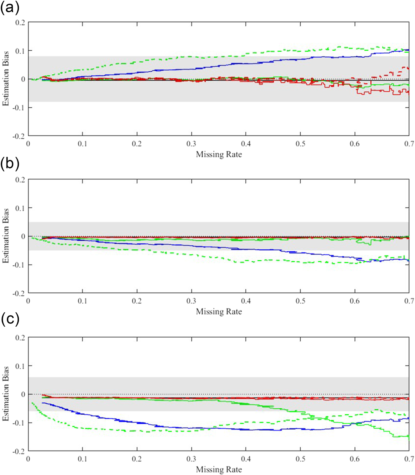
Estimation bias under different missing rate with n = 200: Comparison of methods: FULL (Black, solid line), CCA (BLUE, solid line), IPW-I (Green, solid line), IPW-II (Green, dashed line), NN-1 (Red, solid line), and NN-5 (Red, dashed line). Only 1 and 5 neighbors are used for nearest neighbor imputation. (a) Estimation biases of α. (b) Estimation biases of β ₁. (c) Estimation biases of β ₂.

6 An application

Now we apply the methodology proposed in the previous sections to the ADNI data discussed before. In the study, the participants are classified into three groups, cognitively normal (CN), mild cognitive impairment (MCI) and Alzheimer’s disease (AD). As discussed above, one of the variables of interest is the onset of AD conversion, and given the nature of the study, only interval-censored data are available on it. More specifically, the onset is only known to fall within the interval between the last observation time when the conversion had not occurred and the first observation time when it had already occurred.

In the analysis below, following others [30], 31], we will focus on the participants in the MCI group with the goal of determining the relationship between the time from the baseline visit date to AD conversion, the failure time of interest, and eight covariates. These covariates are AGE, GENDER, two AD assessment scale test results (ADAS11 and ADAS13), middle temporal gyrus volume (MIDTEMP), Rey Auditory Verbal Learning Test score of immediate recall (RAVLT), functional assessment questionnaire score (FAQ), and APOE4, a gene widely known to be related to AD. The dataset consists of 383 subjects with 213 converting to AD during the study.

In general, individuals were scheduled for follow-up examinations approximately every six months, although some visits were missed. Of the 383 participants, 170 were lost to follow-up before a recorded AD conversion. According to information from the ADNI website, 34 participants died during the follow-up period. Among them, 21 had been diagnosed with AD prior to death, while 13 had not. For ease of interpretation, we introduced a dummy variable based on the following criteria: individuals were categorized as aged 75 and above or below 75. In addition, approximately 20 % or 76 of the MIDTEMP values are missing and there are also three missing values on each of ADAS13 and FAQ. For simplicity, we will exclude the six subjects with missing values on ADAS13 or FAQ.

A more comprehensive summary of the eight covariates used in the analysis is provided in Table 4.

Tables 5 and 6 present the analysis results given by the proposed approach, IPW approach and CCA approach under the PH and PO models. For the IPW approach, the logistic regression was used to model the missing probabilities and we considered two situations, setting W = Z as the covariate (IPW-I) or W = ( Z T , L , R ) T as the covariate (IPW-II). The standard errors of IPW were estimated based on 300 bootstrap samples. For the proposed approach, different neighborhood set sizes (1, 5, and 10) and different values of ω ₁ (0.8, 0.5, and 0.3) were considered. The degree of Bernstein polynomials m = 3 was used in the estimation procedure.

One can see from Tables 5 and 6 that all methods suggested that the factors ADAS13, MIDTEMP, RAVLT, FAQ and APOE4 were significant predictors of the AD conversion. More specifically, it seems that the AD conversion was negatively correlated with MIDTEMP and RAVLT but positively related to ADAS13, FAQ, and APOE4. In addition, all methods also indicated that the factors GENDER and ADAS11 had no significant effects on AD conversion. On the factor AGE, all of the proposed methods suggest that it did not have a significant effect on the AD conversion but both the CCA and IPW approaches overestimated its effect and indicated that it was negatively significantly related to the AD conversion. In other words, contrary to the common belief, they suggest that older subjects had a lower risk of AD conversion. A possible explanation for this is that the resulting estimates are seriously biased. Note that as mentioned above, the results on the factor MIDTEMP, which suffers missing values, are consistent across all methods. This may be because of its extremely significant effects.

As pointed out by a reviewer, our current analysis does not account for death as a competing risk under interval censoring. Since the number of such cases is small, as noted earlier, we believe this limitation is unlikely to affect the main conclusions. Nonetheless, it would be valuable to consider this aspect in future work [32].

7 Discussion and concluding remarks

In this paper, we discussed regression analysis of interval-censored failure time data arising from semiparametric transformation models in the presence of missing covariates. For the problem, we proposed a novel nonparametric multiple imputation procedure by integrating multiple imputations with the sieve maximum likelihood estimation. The method makes use of two predictive scores for each individual and then a neighborhood set for imputations. An extensive simulation study was performed and indicates that the proposed approach performs well and can yield better and more efficient estimators than the complete-case analysis and IPW methods in general.

It is noteworthy that the proposed estimation procedure relies solely on simple maximum likelihood regression, rendering it computationally straightforward. This sets it apart from the existing literature on MAR and general interval-censored data, which entails a more intricate formulation [16]. In particular, the approach given in Zhou et al. [16] involves calculating expected values for missing covariates, introducing significant complexity, especially when handling multiple covariates with missing values and requiring the computation of high-dimensional integrals. Despite incorporating multiple imputation steps, the proposed procedure maintains a swift calculation speed, making it easily implementable using existing packages in standard software such as the icenReg package in R [33]. Furthermore, we extended the proportional hazards model utilized in Zhou et al. [16] to a much broader class of semiparametric transformation models.

In the preceding sections, the focus has been on semiparametric transformation models. However, it should be straightforward to generalize the idea to other models such as the additive hazards models and Cox-Aalen models. Also in the above, we have assumed the independent or non-informative interval censoring and sometimes one may face informative censoring [34], 35]. The idea discussed above can be generalized to this latter situation too but may not be straightforward. For example, with informative interval censoring, one usually needs to model or formulate the censoring mechanism.

Another important assumption made above is that the missing mechanism is MAR or the missingness depends solely on the observed values. It is apparent that sometimes one may encounter more complex mechanisms where the missingness could be related to both observed and missing values, which is usually referred to as nonignorable missing or missing not at random [36]. It would be useful to generalize the proposed method to such situations.

References

1. Sun, J. The statistical analysis of interval-censored failure time data. New York: Springer; 2006.Search in Google Scholar
2. Sun, J, Chen, D. Emerging topics in modeling interval-censored survival data. Switzerland: Springer Nature; 2022.10.1007/978-3-031-12366-5Search in Google Scholar
3. Kalbfleisch, JD, Prentice, RL. The statistical analysis of failure time data. Hoboken: John Wiley & Sons; 2011.Search in Google Scholar
4. Fine, J, Ying, Z, Wei, L. On the linear transformation model for censored data. Biometrika 1998;85:980–6.10.1093/biomet/85.4.980Search in Google Scholar
5. Chen, K, Jin, Z, Ying, Z. Semiparametric analysis of transformation models with censored data. Biometrika 2002;89:659–68. https://doi.org/10.1093/biomet/89.3.659.Search in Google Scholar
6. Zhang, Z, Zhao, Y. Empirical likelihood for linear transformation models with interval-censored failure time data. J Multivariate Anal 2013;116:398–409. https://doi.org/10.1016/j.jmva.2013.01.003.Search in Google Scholar
7. Zeng, D, Mao, L, Lin, D. Maximum likelihood estimation for semiparametric transformation models with interval-censored data. Biometrika 2016;103:253–71. https://doi.org/10.1093/biomet/asw013.Search in Google Scholar PubMed PubMed Central
8. Zhou, Q, Hu, T, Sun, J. A sieve semiparametric maximum likelihood approach for regression analysis of bivariate interval-censored failure time data. J Am Stat Assoc 2017;112:664–72. https://doi.org/10.1080/01621459.2016.1158113.Search in Google Scholar
9. Weiner, MW, Veitch, DP, Aisen, PS, Beckett, LA, Cairns, NJ, Green, RC, et al.. The alzheimer’s disease neuroimaging initiative: a review of papers published since its inception. Alzheim Dement 2013;9:e111–e1 https://doi.org/10.1016/j.jalz.2013.05.1769.Search in Google Scholar PubMed PubMed Central
10. Weiner, MW, Veitch, DP, Aisen, PS, Beckett, LA, Cairns, NJ, Cedarbaum, J, et al.. Impact of the alzheimer’s disease neuroimaging initiative, 2004 to 2014. Alzheim Dement 2015;11:865–84. https://doi.org/10.1016/j.jalz.2015.04.005.Search in Google Scholar PubMed PubMed Central
11. Little, A, Rubin, DB. Statistical analysis with missing data. New York: Wiley; 2002.10.1002/9781119013563Search in Google Scholar
12. Hsu, C-H, Yu, M. Cox regression analysis with missing covariates via nonparametric multiple imputation. Stat Methods Med Res 2019;28:1676–88. https://doi.org/10.1177/0962280218772592.Search in Google Scholar PubMed PubMed Central
13. Lou, Y, Ma, Y, Du, M. A new and unified method for regression analysis of interval-censored failure time data under semiparametric transformation models with missing covariates. Stat Med 2024a;43:2062–82. https://doi.org/10.1002/sim.10035.Search in Google Scholar PubMed
14. Wen, C-C, Lin, C-T. Analysis of current status data with missing covariates. Biometrics 2011;67:760–9. https://doi.org/10.1111/j.1541-0420.2010.01505.x.Search in Google Scholar PubMed
15. Li, H, Zhang, H, Zhu, L, Li, N, Sun, J. Estimation of the additive hazards model with interval-censored data and missing covariates. Can J Stat 2020a;48:499–517. https://doi.org/10.1002/cjs.11544.Search in Google Scholar
16. Zhou, R, Li, H, Sun, J, Tang, N. A new approach to estimation of the proportional hazards model based on interval-censored data with missing covariates. Lifetime Data Anal 2022;28:335–55. https://doi.org/10.1007/s10985-022-09550-y.Search in Google Scholar PubMed
17. Long, Q, Hsu, C-H, Li, Y. Doubly robust nonparametric multiple imputation for ignorable missing data. Stat Sin 2012;22:149. https://doi.org/10.5705/ss.2010.069.Search in Google Scholar
18. Turnbull, BW. The empirical distribution function with arbitrarily grouped, censored and truncated data. J Roy Stat Soc B 1976;38:290–5. https://doi.org/10.1111/j.2517-6161.1976.tb01597.x.Search in Google Scholar
19. Rubin, DB. Inference and missing data. Biometrika 1976;63:581–92. https://doi.org/10.2307/2335739.Search in Google Scholar
20. Little, RJ, Rubin, DB. Statistical analysis with missing data. Hoboken: John Wiley & Sons; 2019.10.1002/9781119482260Search in Google Scholar
21. Allison, P. Missing data. Thousand Oaks, CA: Sage; 2001.Search in Google Scholar
22. Du, M, Lou, Y, Sun, J. Estimation and variable selection for interval-censored failure time data with random change point and application to breast cancer study. J Am Stat Assoc 2025:1–12. https://doi.org/10.1080/01621459.2024.2441522.Search in Google Scholar
23. White, IR, Royston, P. Imputing missing covariate values for the cox model. Stat Med 2009;28:1982–98. https://doi.org/10.1002/sim.3618.Search in Google Scholar PubMed PubMed Central
24. Heitjan, D F, Little, R J. Multiple imputation for the fatal accident reporting system. J Roy Stat Soc Series C Appl Stat 1991;40:13–29. https://doi.org/10.2307/2347902.Search in Google Scholar
25. Lou, Y, Ma, Y, Xiang, L, Sun, J. A multiple imputation approach for flexible modelling of interval-censored data with missing and censored covariates. Comput Stat Data Anal 2025:108177. https://doi.org/10.1016/j.csda.2025.108177.Search in Google Scholar
26. Nielsen, SF. Proper and improper multiple imputation. Int Stat Rev 2003;71:593–607. https://doi.org/10.1111/j.1751-5823.2003.tb00214.x.Search in Google Scholar
27. Rubin, D B. Multiple imputation for nonresponse in surveys. New York: John Wiley & Sons; 1987.10.1002/9780470316696Search in Google Scholar
28. Huang, J, Rossini, A. Sieve estimation for the proportional-odds failure-time regression model with interval censoring. J Am Stat Assoc 1997;92:960–7. https://doi.org/10.2307/2965559.Search in Google Scholar
29. Chen, D-GD, Sun, J, Peace, KE. Interval-censored time-to-event data: methods and applications. Boca Raton: CRC Press; 2012.10.1201/b12290Search in Google Scholar
30. Li, K, Chan, W, Doody, RS, Quinn, J, Luo, S, Initiative, ADN, et al.. Prediction of conversion to alzheimer’s disease with longitudinal measures and time-to-event data. J Alzheim Dis 2017;58:361–71. https://doi.org/10.3233/jad-161201.Search in Google Scholar
31. Li, S, Wu, Q, Sun, J. Penalized estimation of semiparametric transformation models with interval-censored data and application to alzheimer’s disease. Stat Methods Med Res 2020b;29:2151–66. https://doi.org/10.1177/0962280219884720.Search in Google Scholar PubMed
32. Leffondré, K, Touraine, C, Helmer, C, Joly, P. Interval-censored time-to-event and competing risk with death: is the illness-death model more accurate than the cox model? Int J Epidemiol 2013;42:1177–86. https://doi.org/10.1093/ije/dyt126.Search in Google Scholar PubMed
33. Anderson-Bergman, C. icenreg: regression models for interval censored data in r. J Stat Software 2017;81:1–23. https://doi.org/10.18637/jss.v081.i12.Search in Google Scholar
34. Du, M, Zhou, Q. Analysis of informatively interval-censored case-cohort studies with application to hiv vaccine trials. Commun Math Stat 2023;13:195–215. https://doi.org/10.1007/s40304-022-00322-6.Search in Google Scholar
35. Lou, Y, Sun, J, Wang, P. Semiparametric cure regression models with informative case k interval-censored failure time data. Stat Sin 2026;36:1–22.10.5705/ss.202022.0343Search in Google Scholar
36. Du, M, Li, H, Sun, J. Regression analysis of censored data with nonignorable missing covariates and application to alzheimer disease. Comput Stat Data Anal 2021;157:107157. https://doi.org/10.1016/j.csda.2020.107157.Search in Google Scholar
Supplementary Material
This article contains supplementary material (https://doi.org/10.1515/ijb-2024-0016).
© 2025 Walter de Gruyter GmbH, Berlin/Boston
Articles in the same Issue
- Frontmatter
- Research Article
- The gROC curve and the optimal classification
- Review
- Leveraging external information by guided adaptive shrinkage to improve variable selection in high-dimensional regression settings
- Research Articles
- Enhanced doubly robust estimate with semiparametric models for causal inference of survival outcome
- Two-sample empirical likelihood method for right censored data