GAMLSS for high-variability data: an application to liver fibrosis case

1 Introduction

In many applicative studies, the average level of certain response variables cannot be controlled unless variability in its measurements is previously reduced. This happens very often in medical studies when the interest lies in determining the presence of some diseases and the relevant level of progression, through the use of some laboratory measurements. Those are characterized by high-variability between observations and no gold standard exists; or, alternatively, when repeated measurements with high-variability are available for the same patient. In both cases, it is essential to know the within-subject variability in order to establish the presence of the disease. Clinicians must understand variability in measurements both qualitatively and quantitatively and endeavour to reduce that variability before trying to use data to establish a patient’s health condition.

In fact, when data exhibit high-variability, any model fit in order to derive an average behaviour of the phenomenon under study will be characterized by “overdispersion” [1]. When it is not possible to eliminate variability before analysing the data, it will result in a substantial discrepancy in variance, which constitutes evidence of an inadequate model fit for the high-frequency variations in the outcome. In this regard, [2], [3] obtained results suggesting that the extent of overdispersion can be reduced, but not necessarily eliminated, by fitting more complex stochastic models that better reflect the nature of the observed extra-variability. In this paper, we propose management of the problem caused by overdispersed data by applying the generalized additive model for location, scale and shape framework (GAMLSS) as introduced by [4]. The idea of using a GAMLSS approach for handling our problem comes from the idea of [5] consisting in the use of an EM maximum likelihood estimation algorithm [6] to deal with overdispersed generalized linear models (GLM). As in the GLM case, the algorithm is initially derived as a form of Gaussian quadrature assuming a normal mixing distribution. The GAMLSS specification allows the extension of the Aitkin algorithm to probability distributions not belonging to the exponential family. In particular, aim of this work is to show the importance of using a GAMLSS strutcure when a mixture is used to provide a natural representation of heterogeneity in a finite number of latent classes [7].

From an applicative point of view, the need for the specification of a GAMLSS able to deal with overdispersed data comes from the analysis of Liver fibrosis data. In the Liver fibrosis data, the response variable is liver stiffness measured as wave speed (expressed in m/s) registered by the Acoustic Radiation Force Impulse (ARFI), while the explanatory variables are divided into two groups: patient-specific explanatory variables (sex, age, size and weight) and explanatory variables relevant to the exam (depth, liver segment, patient position). As Figure 1 shows, wave speed data seem to exhibit overdispersion. In particular, data show a variance increasing with the mean (A) and a non-linear relationship between means and the log transformed variances (B) is observed. In this work, the use of a finite mixture model for GAMLSS will be proposed as a solution to the problem of multimodality in determining the presence of liver diseases and to establish its level of severity.

Figure 1:

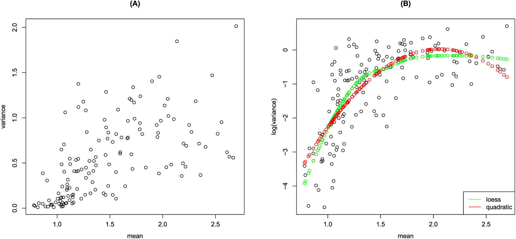
Mean-variance (A) and mean-log(variance) (B) relationships in Liver fibrosis data, in green a fitted curve for loess, in red a fitted curve for quadratic.

The paper is structured as follows: after a brief review of GAMLSS theory (Section 2), an extension of the finite mixture framework to the class of GAMLSS is introduced in Section 3. Section 4 is devoted to an application of the proposed approach to Liver fibrosis data. Some simulation results are reported in Section 5 before presenting our conclusions.

2 GAMLSS modelling: a real application

General Additive Models for Location Scale and Shape were introduced firstly by [8] as a way of overcoming some of the limitations associated with Generalized Linear Models [9] and Generalized Additive Models [10]. They represent a flexible class of models for several reasons. Firstly, they allow the response variable to be selected in a very general family of distributions D including highly skewed and kurtotic continuous and discrete distributions. Moreover, they are a flexible class of models because, once the response distribution has been fixed, all the parameters characterizing the chosen distribution can be modelled by using parametric and/or non-parametric smooth functions of the explanatory variables (i. e. cubic splines, penalized splines, lowess) and/or random effects. Thus, assuming the response variable Y follows a four-parameter distribution Y ∼ D ( θ ) with θ = ( μ , σ , ν , τ ) , where µ and σ are usually location and scale parameters, while ν and τ shape parameters, the formulation of GAMLSS given by [4] is:

where X k is a known fixed effects design matrix of order n × J ′ k , g k ( . ) are known monotonic link functions relating, in a parametric way, the distribution parameters to the explanatory variables X k and h j k represent the non-parametric additive terms. The model in Equation (1) can be extended to allow for the inclusion of non-linear parametric terms in the model, for μ , σ , ν and τ, as discussed in [11]. The vector of parameters β k and the non-parametric terms h j k are estimated by maximizing a penalized likelihood function l p defined as the difference between the log likelihood function of the distribution parameters given the data l = ∑ ​ i = 1 n l o g f Y ( y i | θ i ) = ∑ ​ i = 1 n l o g f Y ( y i | μ i , σ i , ν i , τ i ) and a quadratic penalty term which depends on fixed hyperparameters λ . The penalized log-likelihood l p can be estimated following two basic algorithms. The first one, the CG algorithm, is a generalization of the [12] algorithm that uses the first derivatives and the expected values of the second and cross derivatives of the likelihood function with respect to θ = ( μ , σ , ν , τ ) for a four-parameter distribution. However, for many probability (density) functions, f Y ( y | θ ) , the θ parameters are information orthogonal. In this case, the simpler RS algorithm that does not use the cross derivatives is more suitable. The RS algorithm is a generalization of the algorithm used by [13], [14] for fitting Mean And Dispersion Additive Models (MADAM). Details about the algorithms used to maximize the penalized log likelihood l p can be found in [15]; an application of GAMLSS on Liver fibrosis data is shown below.

Liver fibrosis is one of the 10 most frequent causes of death in the world and consists of excessive accumulation of extracellular matrix proteins, including collagen, which occurs in most types of chronic liver diseases. Advanced liver fibrosis can result in cirrhosis, liver failure, and portal hypertension and often requires liver transplantation [16]. The severity of liver fibrosis can be classified in five stages, based on the Metavir scoring system, from a normal (F0) to a cirrhotic (F4) liver [17]. In medicine, liver biopsy represents the gold standard test for staging liver disease [18]. An alternative diagnostic technique is represented by the Acoustic Radiation Force Impulse (ARFI) [19].

ARFI measures liver stiffness through mechanical excitation of tissue, using acoustic pulses producing shear wave propagation. According to the ARFI principle, the stiffer the tissue, the faster shear waves will propagate. The dataset used in this example consists of ARFI measurements taken in 2013 from 141 patients. As during each elastography, several measurements are gathered, the dataset has a two-step hierarchical structure: a macro “exam level” and a second nested level for the measurements taken during the same exam. The response variable is liver stiffness measured as wave speed (expressed in m/s) registered by ARFI, while the explanatory variables are divided into two groups: patient-specific explanatory variables (sex, age, size and weight) and explanatory variables relevant to the exam (depth, liver segment, patient position).

Since hepatic fibrosis affects the liver patchy, the advantage of obtaining repeated measurements from different parts of liver becomes fundamental. The possibility of obtaining depth data represents the most important innovation of this dataset since data on depth is available for the first time. ARFI allows to measure liver stiffness at different depths starting from 1.5 cm to a maximum of 8 cm. Understanding how wave speed changes when stiffness is measured at different depths represents a very important objective of this study. Moreover, as liver is divided into segments, a four-level (Segment = 5, 6, 7, 8) factor variable has been included in the dataset. Some studies in the literature show how the position of a patient during the examination affects the value of wave speed measured by ARFI [20], [21]. Liver fibrosis data also include information about patient positions: supine (ant), lateral (lat) and prone (pos).

The complexity of the dataset, together with the overdispersion already shown in Figure 1, has led us to consider not only modelling of the location parameter but also use of GAMLSS object in order to provide a structure to the other parameters characterizing the assumed response variable distribution. Among the more than 80 distributions implemented in GAMLSS, we have to search for a continuous and positive skewed distribution in R+ taking kurtosis also into account. Six probability distributions have been selected, and a null model has been fitted for the reduced dataset. In particular, we fitted the following probability distributions: IG (Inverse Gaussian) [22]; BCCG (Box–Cox Cole and Green) [12]; BCPE (Box-Cox Power Exponential) [23]; BCT (Box–Cox generalized t) [11]; GB2 (Generalized Beta 2) [24]; ex-GAUS (exponentially modified Gaussian (EMG) distribution) [25]. The choice of a suitable distribution for the ARFI speed variable relapsed on the Box–Cox Power Exponential (BCPE) distribution. It was introduced by [23] in order to model both skewness and kurtosis in the distribution of a continuous response variable Y.

Once the response variable distribution has been properly specified, the GAMLSS model is selected by comparing various competing models in which different combinations of the components of the model are used. Thus, for example, a set G of link functions ( g 1 , g 2 , g 3 , g 4 ) for the four parameters in θ has to be properly specified. A set of linear predictor terms has to be defined for the four parameters of the assumed response distribution. Selection of the predictor terms can be considered the biggest problem for the model selection procedure due to the high number of variables involved in a linear system of four equations. Moreover, the hierarchical structure of data and the presence of repeated measurements suggest the inclusion of some random effects in order to account for the correlation between observations on the same patient. Therefore, another important aspect in model selection is the inclusion of hyperparameters in the model. The specification of all these components will be based on a measure of global goodness of fit used to compare several models. Each GAMLSS fitted model is generally assessed by using its Global Deviance (GD) given by G D = − 2 l p ( θ ^ ) where l p ( θ ^ ) = ∑ ​ i = 1 n l p i ( θ ^ ) . Two nested models M 0 and M 1 will be compared by using the test statistic Λ = G D 0 − G D 1 which has an asymptotic χ 2 -distribution under M 0 with d = d f M 0 − d f M 1 degrees of freedom. When comparing non-nested GAMLSS, the Generalized Akaike Information Criterion (GAIC) [26] can be used to penalize overfittings. GAIC is obtained by adding a fixed penalty term p to the fitted global deviances, for each effective degree of freedom used in the model ( p = 2 corresponds to the standard Akaike Information Criterion [26], while p = log n is the Bayesian Information Criterion [BIC] [27]).

The model with the smallest GAIC value will be selected. Several GAMLSS models have been fitted to Liver fibrosis data. A grid of penalty values p has been checked, and the respective number of explanatory variables included in the model for each parameter ( μ , σ , ν , τ ) is displayed in Table 1. A penalty p = l o g ( n ) = 8.32 has been chosen looking for a satisfactory trade-off between simplicity of the model and loss of information.

Once the value p for the penalty has been selected, we tried to use a modified version of BCPE distribution using a log link function for parameter µ of the model. Finally, in order to account for the correlation between observations measured on the same patient, a random effect component for the patient grouping factor was included. The selected final model is shown below:

where 1 | p a t i e n t stands for the random effect for the single patient. Results from the fitted model are reported in Table 2.

Age seems to be the most important predictor for wave speed since it enters each equation of the selected model. Its estimated value is positive for all the equations. On the contrary, depth has a negative effect on wave speed; in particular, a unitary increase in depth produces, on average, a 5% decrease ( 1 − e x p ( − 0.048 ) ) in the mean value of wave speed. Segment is significant only for the µ parameter with Segment 5 (baseline) not significantly different from Segment 6. Segment 7 is highly different from baseline with wave speed for Segment 7, on average, 12% ( 1 − e x p ( − 0.128 ) ) lower than that in baseline; the estimated value for Segment 8 is positive with an average effect on the logarithm of speed equal to e x p ( 0.075 ) = 1.077 . For the scale parameter σ, four variables are significant. The negative coefficient for size (the patient height) is an interesting result: when size increases by 1 cm, the variability in wave speed seems to decrease 0.6% ( 1 − e x p ( − 0.920 ) ). No significant differences in variability exist between anterior and lateral positions, while the posterior position results are significantly different with a variability in posterior wave measurements that is 14% higher than for observations in the anterior one. For skewness and kurtosis, the only significant terms are negative intercepts and positive coefficients for age.

3 Mixture models in GAMLSS

When conducting any statistical analysis, it is important to evaluate how well the model fits the data and whether the data meet the assumptions of the model. There are numerous ways to do this and a variety of statistical tests to evaluate deviations from model assumptions. Generally, once a model is fitted, the overall adequacy of the selected model is assessed through the analysis of residuals by using both diagnostic plots and tests. Within the framework of GAMLSS, the analysis of residuals is based on the use of randomized quantile residuals. This class of residuals has been introduced by [28] for regression models with independent responses. They are defined as the standard normal quantiles corresponding to the inverse of the fitted distribution function evaluated for each response value. In particular, let us assume that F ( y ; μ , ϕ ) is the cumulative distribution function of P ( μ , ϕ ) . If F is continuous, then the F ( y i ; μ i , ϕ ) are uniformly distributed on the unit interval. In this case, the quantile residuals are defined by

where Φ ( ⋅ ) represents the cumulative distribution function of the standard normal distribution. Such residuals can also be derived when the response variable is discrete, by including a number of randomization procedures in order to ensure continuous residuals. Dunn and Smyth [28] have shown that such a definition produces residuals that are exactly normal, apart from sampling variability in the estimated parameters. Since the properties of residuals are known, a graphic representation of the quantile residuals against the predictors could represent a diagnostic tool capable of identifying regions of explanatory variables within which the models do not show an adequate fit. In this work, among the several graphical diagnostic tools proposed in the literature, we propose the use of the worm plot of residuals introduced by [29]. The worm plot consists of a number of detrended Q–Q plots split according to certain predictors. In particular, the vertical axis of a worm plot portrays, for each observation, the difference between its location in the theoretical and empirical distributions. The data points in each plot form a worm-like string. The shape of the worm indicates how the data differ from the assumed underlying distribution. A model that fits the data well is characterized by a “flat worm”. The 95 per cent confidence interval is plotted as well in order to delineate the region where the worm should be located most of the times, provided the empirical and theoretical distributions agree.

In a GAMLSS context, worm plots are largely used to derive hints about the positions where the GAMLSS fit needs to be improved, but also to identify particular features in the data [30], such as overdispersion or multimodality. Liver fibrosis data, from a first descriptive analysis, appear to be characterized by high variability; in particular, the worm plot relevant to the selected model, which is summarized in Equation (2) (Figure 2 (A)) exhibits an M-shape pattern that requires improvement in the specified parametric model. In fact, as extensively discussed in the literature, when inadequately modelled, heterogeneity can lead to underestimation of the standard errors of regression parameters, too narrow confidence intervals and too small p-values [5], [31].

Figure 2:

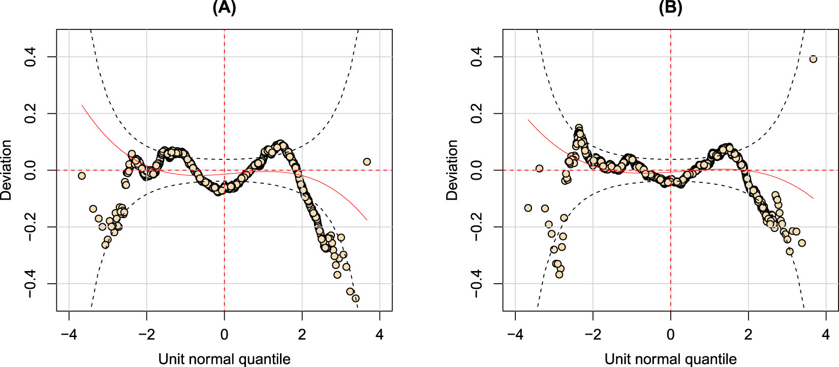
Worm plots for two fitted GAMLSS objects: (A) the worm plot of the BCPEo GAMLSS in Equation (2); (B) the worm plot of the GAMLSS with a finite mixture distribution for the response.

When heterogeneity is due to the presence of subpopulations within an overall population, then a mixture model could be the best solution for representing the probability distribution of observations in the overall population. There is an extensive amount of literature on mixture distributions and their use in modelling data [32], [33], [34], [35]. Yet, the use of mixture distributions for GAMLSS represents a complex and interesting area of research for this class of models.

The aim of this paper is to suggest the use of a mixture approach for GAMLSS when, as in the Liver fibrosis example, data exhibit heterogeneity. The central idea is that the M-shaped pattern in the worm plots could be the result of a spurious appearance of a bimodal distribution. Therefore, the use of a GAMLSS mixture model could be useful for proper identification of the underlying distribution. Thus, as in a standard finite mixture model, let us assume that the response variable Y follows a distribution f that is a mixture of R component distributions f 1 , f 2 , … , f R :

where each component contributes to the total density with weights π r , being the mixing weights, π r > 0 , ∑ r π r = 1 . The natural way to introduce finite mixture distributions in a GAMLSS framework consists in assuming that all the R components of the mixture are represented by GAMLSS models. Moreover, according to the assumptions about the parameters involved in each R component, it is possible to distinguish two different specifications of finite mixture models in GAMLSS [36]. The first one assumes that each density function f r ( y ) depends on a set of parameters θ r with no parameters in common with two or more parameter sets.

This assumption allows the use of different GAMLSS distributions for each conditional distribution component f r ( y ) in the mixture. Alternatively, the second approach allows the R components of the mixture to have parameters in common, that is the parameter sets ( θ 1 , θ 2 , … , θ R ) are not disjoint. Note that since some of the parameters may be common to the R components, the distribution used and the assumed link functions must be the same for all components. An important issue, valid for both the specifications discussed above, is the dependence of the mixing weights on a number of explanatory variables. The possibility to use non constant mixing weights can be applied in all situations where the probability of belonging to one of the R sub-populations could depend on exogenous variables (healthy status, age, exposure to some agents, etc.). However, it is specified that maximization of the likelihood function of a finite mixture model in GAMLSS is carried out using an EM algorithm [6]. The R package gamlss.mx enables fitting of mixtures of distributions with estimated weights, which can also depend on covariates. Figure 2 (B) represents the worm plot for the GAMLSS with predictor terms as in Equation (2) but with the BCPEo replaced by a finite mixture. The comparison of the two worm plots shows the gain in goodness of fit derived from the use of the mixture. The worm becomes flatter and a fewer number of points fall out of the 95 per cent confidence intervals.

4 Mixture GAMLSS and Liver fibrosis: results

As already discussed in the previous Section, the comparison between the worm plots obtained by the two properly specified GAMLSS fits seems to confirm the hypothesis about a bimodality in Liver fibrosis data that could justify the observed high variability. From a medical point of view, a possible explanation of this bimodality is that the two components in the mixture could represent two classes of subjects: healthy and cirrhotic patients.

Once the proposed finite mixture GAMLSS has been fitted, it is possible to derive the estimated posterior probabilities pertaining to the two mixture components for each statistical unit. If the fitted model works well, a correspondence between the estimated probabilities of belonging to a specific sub-population and the objective classification represented by the Metavir score is desired. In order to assess the aforementioned relationship, a graphical representation of the estimated probabilities versus the observed values of speed can be useful. According to the Metavir classification, liver fibrosis is divided into five stages, from F0 to F4, on the basis of the presence of connective tissue in the liver. For simplicity purposes, a three-group classification is used here, as proposed in [20]: F0–F1 (normal liver), F2–F3 (mild fibrosis) and F4 (cirrhosis). The pattern of the scatter plot (Figure 3) suggests a three-category classification for the estimated probabilities, with thresholds derived by visual inspection. By crossing both the categorized variables, a 9-sectors grid is obtained and it is noted that measurements fall within certain specific sectors only. Therefore, this result confirms the hypothesis of a direct relationship between the posterior probabilities and the Metavir staging system, and emphasizes the advantage of using a mixture GAMLSS model for this type of data. In particular, speed values in the category F 0 − F 1 have a 0–69% probability of belonging to the first component of the mixture. The estimated probability reaches the 90% for measurements belonging to cirrhotic patients ( F 4 ). A 3-by-3 table (see Table 3) has been derived from the graph to summarize the results in a quantitative way. Considering all the n = 4129 measurements, the table contains the frequencies observed in each sector of the grid. It is important to emphasize the presence of four zero-cells in the correspondences matrix that implies a considerable association between speed values and the probabilities of falling within a specific mixture component.

Figure 3:

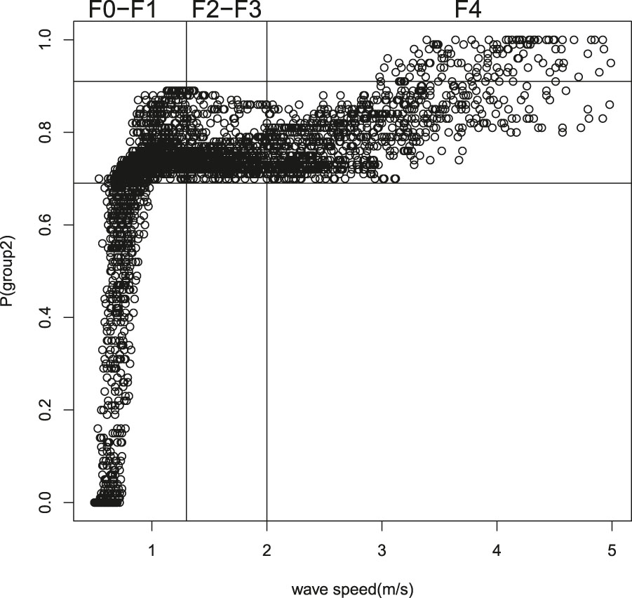
Metavir Stage speed versus mixture posterior probability.

From a medical point of view, this represents an important result because the use of mixture GAMLSS allows to take into account variability in measurements and to derive the disease severity stage through the use of important explanatory variables. Since until now only risk factors have been considered as predictors, it could be also interesting to introduce clinical variables in the dataset. From the existing literature, it is known that laboratory tests play an important role in detecting liver diseases, since anomalous values of alanine transaminase (ALT) and aspartate transaminase (AST) are potential markers of hepatitis. Besides, production of newer serologic markers has been proposed as an aid in determining the degree of liver fibrosis. For this reason, the first clinical variable considered is an indicator variable of anomalous values for the tra ratio index defined as A S T / A L T . Since anomalous values of this index could be symptom related to other liver diseases, an additional clinical variable has been introduced. It is an indicator variable of fibrosing Hepatitis C Virus (HCV). It is based on the diagnosis provided by medical doctors after accurate exams. Like many liver diseases, it is asymptomatic and could culminates in cirrhosis. Thus, high correlation is expected between the presence of HCV and high values of ARFI speed.

The selection model procedure previously described has been implemented including clinical variables and coefficient estimates of the final selected model with the corresponding standard errors are displayed in Table 4. The model has a framework similar to the one in Table 2 except for the clinical variables. Both tra and HCV have an effect on the location parameter with positive coefficients. Moreover, Segment effect is no longer included in the model. Predictor terms for the scale parameter are the same in model 2 while tra has a positive effect on the skewness of the response variable.

Nevertheless, the introduction of clinical variables does not solve the problem of overdispersion. An M-shaped pattern is still present in the worm plot as shown in Figure 4 (A). When a finite mixture is assumed for the response variable an improvement in model fit is again evident Figure 4 (B). Randomized quantile residuals take a flatter worm shape and few points fall out of the 95 per cent confidence intervals.

Figure 4:

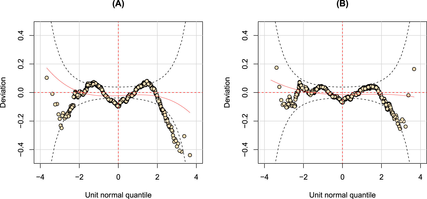
Worm plots for two fitted GAMLSS objects adding clinical variables: (A) the worm plot of the BCPEo GAMLSS in Equation (2); (B) the worm plot of the GAMLSS with a finite mixture distribution for the response.

The conclusions derived from this applicative example show that the processing of data characterized by high-variability cannot be solved by increasing the number of predictor terms in the model. Even the introduction of clinical variables did not help in establishing the severity degree of the disease. Hence, the proposed mixture approach in GAMLSS can be considered the best solution for dealing with overdispersed data.

In Table 5, the estimates of coefficients for the mixture model are presented. It is possible to compare the coefficients tables of the two models: the one in Table 2 and the mixture model one in Table 5. Most of the conclusions derived from the first output are confirmed here. Among predictors, Age is again the most important since it is present in all the equations of the model. Depth has a significant negative effect on Speed. The only liver segment that differs from the baseline (segment 5) is segment 7. As for as log σ is concerned, even in this case there is no significant difference between anterior or lateral position, while the posterior one has a positive effect on the variance. All other coefficients are equally signed and similar in terms of absolute value. Moreover, the new coefficient named MASS is positive and statistically significant. The use of a mixture model is justified and the difference between the two components is positive.

Besides, comparisons between linear GAMLSS and GAMLSS mixture extension are carried out in two ways. Firstly, a comparison in terms of goodness of fit is achieved using Global Deviances (GD). Secondly, the worm plot is used as diagnostic tool and since, according to our hypotheses, the use of a mixture model gets a more flat worm, the h number of points outside the confidence interval bands, is used as criterion for comparison. We wish for a lower GD and a lower h for the mixture model. Mixture model has a lower GD with Δ G D = 34.30 . As we can see from Figure 2, there is a difference between the two worm plots: compared to the one on the left (original model), the second one with the mixture approach is more flat and on the right tail more points are now within the boundaries with a difference of 1355 points.

5 Simulation studies

A number of simulations have been run in order to evaluate the goodness of a mixture approach in GAMLSS when the response variable seems to be bimodal. The starting scenario is very similar to the one in Liver fibrosis data. M = 50 datasets have been simulated with n = 1000 observations. Each dataset includes a response variable Y and three explanatory variables X 1 , X 2 , X 3 . The Y variable is obtained as mixture of two BCPEo distributions with weights of π 1 = 0.75 (the observed proportion of non-cirrhotic patients in the real Liver fibrosis dataset) and π 2 = 0.25 respectively. The three predictors X 1 , X 2 , X 3 are simulated from a normal distribution ( X 1 , X 2 , X 3 ∼ N ( 5,1 ) ). Simulated densities of the two components Y 1 and Y 2 are displayed in Figure 5.

Figure 5:

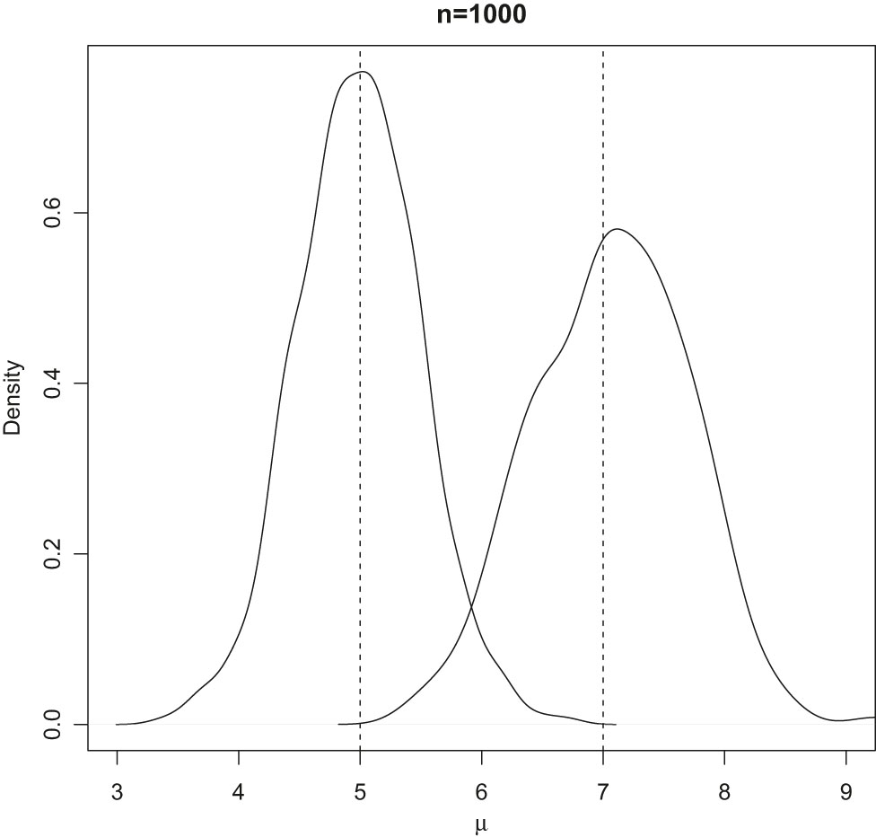
Densities of the two mixture components in Scenario 1.

A GAMLSS involving four parameters ( μ , σ , ν , τ ) has been fitted to these simulated data. The framework used in GAMLSS specification is similar to the final model selected with the real data and it is shown below:

where Y 1 ∼ B C P E o ( 5,0.1 , 1,2 ) and Y 2 ∼ B C P E o ( 7,0.1 , 1,2 ) .

Using the same dataset, a GAMLSS with a finite mixture assumed for the response variable was estimated. Comparisons between standard GAMLSS and the proposed GAMLSS mixture are carried out in two ways. Firstly, a comparison in terms of goodness of fit is achieved using their Global Deviances. Then, worm plots are used as a diagnostic tool. In particular, since according to our hypotheses the use of a mixture model products a flatter worm, the number of points h outside the confidence interval bands is used as a criterion for model comparisons. A lower GD and a lower number of points outside the bandwidths for the mixture model are desirable.

Several scenarios have been simulated by changing a parameter value each time: different mean values for μ 2 have been used in order to check the dependence on the mean values of the selected mixture distributions (scenario 2–5); two different values for the parameter σ 1 relevant to the first BCPEo mixture component have been used σ = 0.25 , 0.5 (scenario 6–7); ν = − 1,0 (scenario 8–9) and τ = 1,3 (scenario 10–11) have been implemented; finally, different weights π 1 for the mixture component have been considered π 1 = 0.5 , 0.9 (scenario 12–13).

Table 6 summarizes all possible scenarios and contains, for each of them, both the average difference in Global Deviance between the standard GAMLSS fit and the model assuming the finite mixture ( Δ G D ¯ ) and the difference between the two fitted models in terms of number of points outside the confidence interval bands ( Δ h ¯ ). Looking at the table, it is possible to note that good results are obtained with the starting scenario characterized by a Δ G D ¯ = 19.4 and a difference in terms of number of points equal to Δ h ¯ = 52 .

Moreover, the table shows that, when the distance between μ 1 and μ 2 decreases, the two approaches appear to be very similar; when this distance increases, the two indicators used for the comparison increase too. When μ 1 and μ 2 are fixed and σ increases (scenario 6–7), the mixture components are flatter and similar results to scenario 2 are obtained where there are no differences between the two approaches. Scenarios for negatively skewed or symmetric distributions (8–9) seem to give better results than the first one. Different values for kurtosis τ = 1,3 (10–11) show that, when low values are selected, the results are similar for both models; instead, when using higher values, the results are similar to scenario 1. Finally, different weights π 1 for the mixing component lead to slight differences between the two fits (12–13).

Similar results are obtained when increasing the number of observations ( n = 2000 ) in the simulated datasets (Table 7). In conclusion, it possible to state that differences in terms of Δ G D ¯ and Δ h ¯ are related to the features of the mixture components: when they do not totally overlap, there is a clear gain in global goodness of fit when using the proposed finite mixture GAMLSS fit rather than the classical GAMLSS approach. On the contrary, when the mixture components are not perfectly separate, the advantage of using a mixture depends on the location and scale parameters of the distributions. Finally, the choice of weights π can also influence the results because opportunely chosen weights allow to weaken roughly high-variability in data.

6 Discussion

The GAMLSS modelling procedures described here are useful for several reasons. First, they prove to be convenient statistical models for dealing with high-variability phenomena. Secondly, they provide information about the relationship between predictive factors, clinical variables and disease risk that is not revealed by the use of standard modelling techniques. GAMLSS could be widely applied to medical research, since high variability and overdispersion are frequently recurring situations when clinical data are analysed. For Liver fibrosis data, a linear GAMLSS model points out that wave speed produced by ARFI is influenced by a number of risk factors. In particular, age of patient, depth and segment of the measurements are the most relevant predictors in the study. In Liver fibrosis data, overdispersion appears when randomized quantile residuals are displayed through the use of worm plots. Specifically, an M-shaped pattern arises and the use of a finite mixture approach in GAMLSS appears to be the best solution for detecting this bimodality. Moreover, a graphical tool is introduced where the estimated posterior probabilities are plotted versus a categorization of wave speed; the resulting pattern confirms the hypothesis that the two identified mixture components are related to the clinical status of the statistical unit. A number of simulation studies have been run in order to evaluate the goodness of a mixture approach in GAMLSS considering similar scenarios for the Liver fibrosis data showing that, when mixture components do not overlap totally, there is a clear gain in global goodness of fit.

Concerning future works, the possibility of solving bimodality problems using this method should be verified through similar datasets and additional simulation studies; this might cover, for example simulated data from other probability distributions, different from the BCPE and data where more than two mixture components are considered.

References

1. Cox, DR. Some remarks on overdispersion. Biometrika 1983;70:269–74. https://doi.org/10.1093/biomet/70.1.269.Search in Google Scholar
2. Kassahun, W, Neyens, T, Faes, C, Molenberghs, G, Verbeke, G. A zero-inflated overdispersed hierarchical poisson model. Statistical Modelling 2014;14:439–56. https://doi.org/10.1177/1471082x14524676.Search in Google Scholar
3. Kassahun, W, Neyens, T, Molenberghs, G, Faes, C, Verbeke, G. A joint model for hierarchical continuous and zero-inflated overdispersed count data. J Stat Comput Sim 2015;85:552–71. https://doi.org/10.1080/00949655.2013.829058.Search in Google Scholar
4. Rigby, RA, Stasinopoulos, DM. Generalized additive models for location, scale and shape. J R Stat Soc Ser C Appl Stat 2005;54:507–54. https://doi.org/10.1111/j.1467-9876.2005.00510.x.Search in Google Scholar
5. Aitkin, M. A general maximum likelihood analysis of overdispersion in generalized linear models. Stat Comput 1996;6:251–62. https://doi.org/10.1007/bf00140869.Search in Google Scholar
6. Dempster, AP, Laird, NM, Rubin, DB. Maximum likelihood from incomplete data via the EM algorithm. J R Stat Soc Ser B 1977; 39:1–38.10.1111/j.2517-6161.1977.tb01600.xSearch in Google Scholar
7. Celeux, G, Diebolt, J. A stochastic approximation type em algorithm for the mixture problem. Stochastics 1992;41:119–34. https://doi.org/10.1080/17442509208833797.Search in Google Scholar
8. Rigby, R, Stasinopoulos, DM. The gamlss project: a flexible approach to statistical modelling. Proceedings of the 16th International Workshop on Statistical Modelling 2001:249–56.Search in Google Scholar
9. Nelder, JA, Wedderburn, RWM. Generalized linear models. J R Stat Soc Ser A 1972;135:370–82. https://doi.org/10.2307/2344614.Search in Google Scholar
10. Hastie, T, Tibshirani, R. Generalized additive models. London: Chapman & Hall; 1990.Search in Google Scholar
11. Rigby, RA, Stasinopoulos, DM. Using the box-cox t distribution in GAMLSS to model skewness and kurtosis. Stat Model 2006;6:209–29. https://doi.org/10.1191/1471082x06st122oa.Search in Google Scholar
12. Cole, TJ, Green, PJ. Smoothing reference centile curves: the LMS method and penalized likelihood. Statistics in Medicine 1992;11:1305–19. https://doi.org/10.1002/sim.4780111005.Search in Google Scholar
13. Rigby, R, Stasinopoulos, D. A semi-parametric additive model for variance heterogeneity. Statistics and Computing 1996a;6:57–65. https://doi.org/10.1007/bf00161574.Search in Google Scholar
14. Rigby, RA, Stasinopoulos, MD. Mean and dispersion additive models. In Statistical theory and computational aspects of smoothing, Springer 1996b:215–30.10.1007/978-3-642-48425-4_16Search in Google Scholar
15. Stasinopoulos, MD, Rigby, RA, Heller, GZ, Voudouris, V, De Bastiani, F. Flexible regression and smoothing: using GAMLSS in R, Chapman and Hall/CRC; 2017.10.1201/b21973Search in Google Scholar
16. Friedman, SL. Liver fibrosis – from bench to bedside. J Hepatol 2003;38:38–53. https://doi.org/10.1016/s0168-8278(02)00429-4.Search in Google Scholar
17. Bedossa, P, Poynard, T. An algorithm for the grading of activity in chronic hepatitis c. Hepatology 1996;24:289–93. https://doi.org/10.1002/hep.510240201.Search in Google Scholar
18. Skelly, MM, James, PD, Ryder, SD. Findings on liver biopsy to investigate abnormal liver function tests in the absence of diagnostic serology. J Hepatol 2001;35:195–9. https://doi.org/10.1016/s0168-8278(01)00094-0.Search in Google Scholar
19. Nightingale, K. Acoustic radiation force impulse (arfi) imaging: a review. Curr Med Imaging Rev 2011;7:328. https://doi.org/10.2174/157340511798038657.Search in Google Scholar
20. Attanasio, M, Enea, M, Rizzo, L. Some issues concerning the statistical evaluation of a screening test: the ARFI ultrasound case. Statistica 2010;70:311–22. https://doi.org/10.6092/issn.1973-2201/3588.Search in Google Scholar
21. Goertz, R, Egger, C, Neurath, M, Strobel, D. Impact of food intake, ultrasound transducer, breathing maneuvers and body position on acoustic radiation force impulse (ARFI) elastometry of the liver. Ultraschall Med 2012;33:380–5. https://doi.org/10.1055/s-0032-1312816.Search in Google Scholar
22. Johnson, NL, Kotz, S, Balakrishnan, N. Continuous univariate distributions. New York: John Wiley & Sons; 1994, vol. 1–2.Search in Google Scholar
23. Rigby, RA, Stasinopoulos, DM. Smooth centile curves for skew and kurtotic data modelled using the box–cox power exponential distribution. Stat Med 2004;23:3053–76. https://doi.org/10.1002/sim.1861.Search in Google Scholar
24. McDonald, JB, YJ Xu. A generalization of the Beta distribution with applications. J Econom 1995;66:133–52. https://doi.org/10.1016/0304-4076(94)01612-4.Search in Google Scholar
25. Grushka, E. Characterization of exponentially modified gaussian peaks in chromatography. Anal Chem 1972;44:1733–8. https://doi.org/10.1021/ac60319a011.Search in Google Scholar
26. Akaike, H. A new look at the statistical model identification. IEEE Trans Autom Control 1974;19:716–23. https://doi.org/10.1109/tac.1974.1100705.Search in Google Scholar
27. Schwarz, G. Estimating the dimension of a model. Ann Stat 1978;6:461–4. https://doi.org/10.1214/aos/1176344136.Search in Google Scholar
28. Dunn, P, Smyth, G. Randomized quantile residuals. J Comput Graph Stat 1996;5:236–44. https://doi.org/10.1080/10618600.1996.10474708.Search in Google Scholar
29. van Buuren, S, Fredriks, M. Worm plot: a simple diagnostic device for modelling growth reference curves. Statistics in Medicine 2001;20:1259–77. https://doi.org/10.1002/sim.746.Search in Google Scholar
30. López, J, Francés, F. Non-stationary flood frequency analysis in continental spanish rivers, using climate and reservoir indices as external covariates. Hydrol Earth Syst Sci 2013;17:3103–42. https://doi.org/10.5194/hess-17-3189-2013.Search in Google Scholar
31. Payne, EH, Hardin, JW, Egede, LE, Ramakrishnan, V, Selassie, A, Gebregziabher, M. Approaches for dealing with various sources of overdispersion in modeling count data: scale adjustment versus modeling. Stat Methods Med Res 2015; 26:1802–23. https://doi.org/10.1177/0962280215588569.Search in Google Scholar
32. Everitt, BS, Hand, DJ. Finite mixture distributions. Monographs on Applied Probability and Statistics. London, New York: Chapman & Hall; 1981.10.1007/978-94-009-5897-5Search in Google Scholar
33. McLachlan, G, Peel, D. Finite mixture models. John Wiley & Sons; 2004.Search in Google Scholar
34. Schlattmann, P. Medical applications of finite mixture models, Springer Science & Business Media; 2009.Search in Google Scholar
35. Titterington, D, Smith, A. Statistical analysis of finite mixture distributions; 1985.Search in Google Scholar
36. Stasinopoulos, D, Rigby, B, Akantziliotou, C. Gamlss: generalized additive models for location scale and shape. R package version, 2–0; 2009.10.32614/CRAN.package.gamlss.addSearch in Google Scholar
© 2020 Andrea Marletta and Mariangela Sciandra, published by De Gruyter, Berlin/Boston
This work is licensed under the Creative Commons Attribution 4.0 International License.
Articles in the same Issue
- Research Articles
- Nonparametric bootstrap inference for the targeted highly adaptive least absolute shrinkage and selection operator (LASSO) estimator
- A Bayesian Framework for Robust Quantitative Trait Locus Mapping and Outlier Detection
- Inference for the Analysis of Ordinal Data with Spatio-Temporal Models
- An iterative algorithm for joint covariate and random effect selection in mixed effects models
- An extended trivariate vine copula mixed model for meta-analysis of diagnostic studies in the presence of non-evaluable outcomes
- Super Learner for Survival Data Prediction
- Model-based random forests for ordinal regression
- A Parametric Bootstrap for the Mean Measure of Divergence
- Derivation of Passing–Bablok regression from Kendall’s tau
- Direct effect and indirect effect on an outcome under nonlinear modeling