
Efficient estimation of pathwise differentiable target parameters with the undersmoothed highly adaptive lasso
-
Mark J. van der Laan
 ,
David Benkeser
,
David Benkeser
 and
Weixin Cai
and
Weixin Cai

Abstract
We consider estimation of a functional parameter of a realistically modeled data distribution based on observing independent and identically distributed observations. The highly adaptive lasso estimator of the functional parameter is defined as the minimizer of the empirical risk over a class of cadlag functions with finite sectional variation norm, where the functional parameter is parametrized in terms of such a class of functions. In this article we establish that this HAL estimator yields an asymptotically efficient estimator of any smooth feature of the functional parameter under a global undersmoothing condition. It is formally shown that the L 1-restriction in HAL does not obstruct it from solving the score equations along paths that do not enforce this condition. Therefore, from an asymptotic point of view, the only reason for undersmoothing is that the true target function might not be complex so that the HAL-fit leaves out key basis functions that are needed to span the desired efficient influence curve of the smooth target parameter. Nonetheless, in practice undersmoothing appears to be beneficial and a simple targeted method is proposed and practically verified to perform well. We demonstrate our general result HAL-estimator of a treatment-specific mean and of the integrated square density. We also present simulations for these two examples confirming the theory.
1 Introduction
We consider the estimation problem in which we observe n independent and identically distributed copies of a random variable with probability distribution known to be an element of an infinite-dimensional statistical model, while the goal is to estimate a particular smooth functional of the data distribution. It is assumed that the target parameter is a pathwise differentiable functional of the data distribution so that its derivative is characterized by its canonical gradient.
A regular asymptotically linear estimator is asymptotically efficient if and only if it is asymptotically linear with influence curve the canonical gradient [1] and a number of general methods for efficient estimation have been developed in the literature. If the model is not too large, then a regularized or sieve maximum likelihood estimator or minimum loss estimator (MLE) generally results in an efficient substitution estimator [2–4]. For a general theory on sieve estimation that also demonstrates sieve-based maximum likelihood estimators that are asymptotically efficient in large models, we refer to [5, 6]. These results generally require a sieve-based MLE that overfits the data (or equivalently, undersmooths the estimated functional parameter) and are only applicable for certain type of sieves [7–10].
An alternative to undersmoothing is to use targeted estimator based on the canonical gradient, such as: the one-step estimator, which adds to an initial plug-in estimator the empirical mean of the canonical gradient at the estimated data distribution [1]; an estimating equations-based estimator, which defines the estimator of the target parameter as the solution of an estimating equation with the estimated canonical gradient as estimating function [11, 12]; and targeted minimum loss-estimation, which updates an initial estimator of the data distribution with an MLE of a least favorable parametric submodel through the initial estimator [13–16]. By using an initial estimator of the relevant parts of the data distribution that converges with respect to L 2-type norm to the truth at a rate faster than n −1/4, such as achieved with the HAL-estimator [17, 18], these three procedures will generally result in an efficient estimator.
In this article we focus on a HAL-MLE, a particular sieve MLE described in [17, 18]. The HAL-MLE is defined as the minimizer of an empirical mean of the loss function (e.g., log-likelihood loss) over a particular class of functions. As such, such estimators could also be referred to as empirical risk minimizers. The particular class over which HAL-MLE minimizes risk are functions that can be arbitrarily well approximated by linear combinations of tensor products of univariate zero order spline-basis functions, but where the L 1-norm of the coefficient vector is constrained. The L 1-norm of the coefficients equals the sectional variation norm of the function [18, 19] so that the HAL-MLE corresponds with minimizing the empirical risk over all cadlag functions with a bound on their sectional variation norm.
The class of k
1-dimensional real-valued cadlag functions with finite sectional variation norm differs from typical smoothness classes that assume pointwise derivatives (e.g., Hölder classes) by assuming a global rather than local constraint. This finite sectional variation norm constraint allows for functions that are discontinuous, but puts a bound on the total variation of the measures generated by the section of the function that sets some of the coordinates equal to the left-origin of its support (a cube). In spite of the constraint, the class of functions with finite section variation norm is reasonably large, including for example any function whose first-order cross derivatives are uniformly bounded. In spite of its size, this class turns out to be a uniform Donsker class with a well-behaved entropy integral. In turn, this Donkser property affords appealing properties of the estimator, such as
The target parameter is defined as a particular smooth real- or Euclidean-valued function of the functional parameter estimated by HAL-MLE, so that the HAL-MLE results in a plug-in estimator of the target parameter. In this case the sieve is indexed by a bound on the L 1-norm. By increasing this bound up to a large, finite value, the sieve includes the total parameter space for the true functional parameter. If the goal is to estimate the functional itself, then the constraint on the L 1-norm is optimally chosen with cross-validation.
In this article we investigate whether and how an appropriately undersmoothed HAL-MLE can be used to produce an efficient plug-in estimator of smooth functions of the functional parameter. There are essentially three key ingredients to establishing efficiency of a plug-in estimator:
negligibility of the empirical mean of the canonical gradient;
control of the second-order remainder; and
asymptotic equicontinuity.
For (i), we argue that since the canonical gradient is a score, we essentially require that HAL-MLE solves a particular score equation. Because HAL-MLE is an MLE, it solves a large class of score equations, and we investigate whether these score equations might also approximate the particular score equation implied by the canonical gradient of the smooth target feature. We find that the larger the L 1-norm of the HAL-MLE, the more such score equations are solved by the HAL-MLE. We also find that the HAL-MLE solves the score equations of paths that ignore the L 1-norm constraint at rate O P (n −2/3), thereby better as the desired o P (n −1/2). Nonetheless, one might need to select a larger L 1-norm than the cross-validation selector to make sure that the basis functions selected by HAL generate enough scores to approximate the desired canonical gradient at the desired precision for the given sample. Either way, by increasing the L 1-norm of the HAL-MLE, the linear span of equations solved by the HAL-MLE will approximate any canonical gradient score equation at the desired precision.
However, in order to satisfy (ii), we must preserve the n −1/4-rate of convergence of achieved by the HAL-MLE, which is naturally achieved when the L 1-norm is selected with cross-validation. Fortunately, the rate of the HAL-MLE is not affected by the size of the L 1-norm as long as it remains bounded and, for n large enough, exceeds the sectional variation norm of the true function. Similarly, the asymptotic equicontinuity condition (iii) will also be satisfied for any bounded L 1-norm, since the class of cadlag functions with a finite sectional variation norm is a Donsker class. In fact, one can prove that this L 1-norm is allowed to slowly converge to infinity as sample size increases without affecting the asymptotic equicontinuity condition and the n −1/4-rate of convergence of the HAL-MLE.
Taken together, our analysis highlights that when selecting the level of undersmoothing of a HAL-MLE, one wants to undersmooth enough to solve the efficient score equation up to an appropriate level of approximation, but in order to reasonable finite-sample performance one should not undersmooth beyond that level. This discussion highlights the need to establish empirical criterion by which the level of undersmoothing may be chosen to appropriately satisfy the conditions required of an efficient plug-in estimator. For that purpose we propose to simply select the L 1-norm till the empirical mean of the canonical gradient is solved at the desired level.
This article is organized as follows. In the next Section 2 we define the HAL-MLE. In Section 3 we establish our main theorem providing the undersmoothing conditions under which the HAL-MLE is asymptotically efficient for any pathwise differentiable parameter. In Section 4 we apply our theorem to the treatment-specific mean example providing a theorem for this particular nonparametric estimation problem. In Section 5 we apply our theorem to a nonparametric estimation problem with target parameter the integrated square of the data density. In Section 6 we demonstrate a simulation study for both examples, providing a practical verification of our theoretical results. We conclude with a discussion in Section 7. Some of the proofs are presented in the Appendices A and B.
2 Defining the functional estimation problem and HAL-MLE
2.1 Functional estimation problem
Suppose we observe
Parameter space for functional parameter
Q
: Cadlag and uniform bound on sectional variation norm. We assume that the parameter space
For a given subset s ⊂ {1, …, k}, Q s : (0 s , τ s ] → IR is defined by Q s (x s ) = Q(x s , 0−s ). That is, Q s is the s-specific section of Q which sets the coordinates in the complement of subset s ⊂ {1, …, k} equal to 0. Since Q s is right-continuous with left-hand limits and has a finite variation norm over (0 s , τ s ], it generates a finite measure, so that the integrals with respect to Q s are indeed well defined. For a given vector x ∈ [0, τ], we define x s = (x(j): j ∈ s). Sometimes, we will also use the notation x(s) for x s .
Note also that
That is, Q(x) is a sum of integrals up to x
s
over all the s-specific edges with respect to the measure generated by the corresponding s-specific section Q
s
. We will refer to Q
s
as a cadlag function as well as a measure. We note that this representation represents Q as an infinitesimal linear combination of indicator basis functions
Note that these basis functions are tensor products over the coordinates j ∈ s of univariate indicator basis functions I(x(j) ≥ u(j)), which are also known as zero-order splines. Note that the L
1-norm of the coefficients in this representation is precisely the sectional variation norm
2.2 Definition of HAL-MLE
Recall
be the HAL-MLE. We will restrict the minimization to Q for which, for all subsets s, dQ
s
(u) is a discrete measure with a finite support {z
s,j
: j = 1, …, n
s
}. That is, for each s, the dQ
s
is absolutely continuous with respect to a discrete counting measure μ
n,s
. We will denote this form of absolute continuity with Q ≪ *μ
n
. In that case, the HAL-MLE is supported by
In this case the HAL MLE can be represented as
and ϕ
j
corresponds with one of the indicator basis functions
As noted earlier, the data adaptive selector C
n
might be selected larger or equal than cross-validation selector
Typically, one is able to prove that the unrestricted MLE (1) will be discrete on a support in which case our μ n -discretization does not restrict the definition of the HAL-MLE. Generally, if O includes observing X where L(Q)(0) depends on Q through Q(X), we recommend to select the support of dQ s as a subset (or whole set) of the observed data X i (s), i = 1, …, n.
3 Efficiency of the HAL MLE for pathwise differentiable target parameters
3.1 Defining the efficient estimation problem and plug-in HAL-MLE
Let
Relevant functional parameter and its loss function: Let
Nuisance parameter for canonical gradient: Let
Here R
20 could have some remaining dependence on P
0 and P, and
Canonical gradient of target parameter in tangent space of loss function: We also assume that this loss function L(Q) is such that there exists a class of submodels
Since the canonical gradient is an element of the tangent space and thereby typically a score of a submodel, this generally holds for Q defined as the density of P and the log-likelihood loss L(Q) = − log Q. However, for any Q there are typically more direct loss functions L(Q), so that the loss-based dissimilarity d 0(Q, Q 0) = P 0 L(Q) − P 0 L(Q 0) directly measures a dissimilarity between Q and Q 0, for which this condition holds as well.
Plug-in HAL-MLE: In this section, we are concerned with analyzing the plug-in estimator Ψ(Q
n
) of Ψ(Q
0), where Q
n
is the C
n
-tuned HAL-MLE
Remark: Target parameter could be component of real target parameter. In many situations the real target parameter is a P → Ψ(Q
1(P), Q
2(P)) for two (or more) functional parameters Q
1 and Q
2. One could apply our efficiency theorem below to the target parameter
this then also establishes asymptotic efficiency of Ψ(Q 1n , Q 2n ) as estimator of Ψ(Q 10, Q 20), under the condition that
This latter term can be viewed as a second order difference of (Q
1n
, Q
2n
) and (Q
10, Q
20) so that the latter condition will generally hold by using the already established rates of convergence
3.2 The HAL MLE solves the unconstrained score-approximation of the efficient influence curve equation by including sparse basis functions
Let
Main idea of result: The HAL-MLE minimizes over a class of functions so that is solves a class of score equations P
n
S
h
(Q
n
) = 0 corresponding with paths
It then remains to approximate the latter
Both of these conditions needed for P n D*(Q n , G 0) = o P (n −1/2) might easily (asymptotically) hold for without any undersmoothing, but either way both will be guaranteed by enough undersmoothing. In practice we find that undersmoothing is important.
The statement of Theorem 1 relies on the following definitions that also provide the basis of the proof of the theorem as outlined above.
Definitions:
Recall we can represent
For notational convenience, we define the extended measure
where we note that ϕ x (u) ≡ I(x ≥ u) reduces to I(x s ≥ u s ) when u is on the edge E s of [0, τ].
Consider the family of paths
(2)Let
For any uniformly bounded h with r(h, Q n ) = 0 we have that for a small enough
Let
Consider the set of scores
(3)where
This is the set of scores generated by the above class of paths if we do not enforce constraint r(h, Q n ) = 0.
We have that Q n solves the score equations P n S h (Q n ) = 0 for any uniformly bounded h satisfying r(h, Q n ) = 0.
Let
We also consider a special case in which
be the set of G’s for which D*(Q n , G) equals a score S h (Q n ) for some uniformly bounded h. One can then define
Let h*(Q n , G 0) be the index so that
Remark: Understanding
As is evident from Theorem 2 below, this approximation G
0n
should aim to approximate G
0 in the sense that R
20(Q
n
, G
0n
, Q
0, G
0) = o
P
(n
−1/2) while also arranging
Convenient notation for finite dimensional spline-representation of Q n : Due to finite support condition Q ≪*μ n in the definition of the HAL-MLE, we have
where ϕ
j
(x) = I(x ≥ u
j
) for the set of indices of all the knot-points {u
j
: j} ⊂ [0, τ], varying over the s-specific edges E
s
of [0, τ] and across the different subsets s ⊂ {1, …, d}. Note β
n
(j) = dQ
n
(u
j
),
The following theorem establishes an undersmoothing condition (5) on C
n
that guarantees
Theorem 1
Consider an approximation
Assume
Then,
Let
and
Regarding (6), if we have
and
Condition (5) is directly verifiable on the data and can thus be used to select the sectional variation norm bound C
n
for the HAL-MLE. For example, one could select a constant a and set C to the smallest value (larger than the cross-validation selector) for which the left-hand side is smaller than
Lemma 1
Consider the special case that O = (Z, X), L(Q)(O) depends on Q through Q(X) only, and
Assume
Then,
The condition (8) can be replaced by
Here P 0 ϕ j and P n ϕ j can be bounded by P 0(X ≥ u j ) and P n (X ≥ u j ), respectively.
Alternatively, we apply Theorem 1 above so that (6) holds if
In [26]; we proved that ∥ Q
n
− Q
0 ∥∞→
p
0 under an absolute continuity condition. However, we expect that the rate of convergence with respect to supremum norm to be close to its rate
3.3 Condition for solving the unconstrained score approximation of the efficient influence curve in terms of number of non-zero coefficients in HAL-MLE fit
Let Q
n
be the HAL-MLE. It solves scores along paths
Let
The following lemma establishes a bound for the latter score equation for z without the orthogonality constraint
Lemma 2
Let J
n
be the number of elements in support
and that, uniformly in z with ∥z∥1 < M for some M < ∞, the random function
We have that for any z/β n < ∞,
Clearly, the first term is o
P
(n
−1/2) as long as J
n
→ ∞. For example, if
Moreover, then
Finally, if for an M < ∞,
Proof
Let z with ∥z∥1 < M and z/β
n
< ∞ be given. We define
In short notation we write
where
We have
Therefore, using that
This completes the proof. □
3.4 Efficiency of the plug-in HAL MLE
The typical general efficiency proof used to analyze the TMLE (e.g., [18]) can be easily generalized to the condition that
Theorem 2
Assume M
1, M
20 < ∞. We have
If
R 2((Q n , G 0n ), (Q 0, G 0)) = o P (n −1/2) and
Otherwise, we assume
R 2((Q n , G 0), (Q 0, G 0)) = o P (n −1/2),
Then, Ψ(Q n ) is asymptotically efficient.
The proof is straightforward, analogue to typical efficiency proof for TMLE, and is presented in the Appendix. Regarding the condition,
However, this equals the P
0-mean of the function
Remark about general impact of undersmoothing on behavior of plug-in HAL-MLE. Though undersmoothing is beneficial for controlling P n D*(Q n , G 0) = o P (n −1/2), it might harm the degree to which the Donsker class condition holds. This puts a clear restriction on the amount of undersmoothing allowed for asymptotic efficiency. The impact of undersmoothing on the second order remainder R 2((Q n , G 0n ), (Q 0, G 0)) is beneficial with respect to the approximation error of G 0 − G 0,n but might make Q n a poor approximation of Q 0. However, in many estimation problems, it appears that undersmoothing reduces the second order remainder as well in the sense that the second order remainder R 2(Q n , G n , Q 0, G 0) can itself be represented as a score P 0 S h (Q n ) for some h, so that undersmoothing reduces the size of the second order remainder. Therefore, undersmoothing may be generally beneficial for the behavior of the estimator as long as its variation norm stays bounded by a universal constant (or a slowly converging constant) as sample size increases.
3.5 Inference for the plug-in undersmoothed HAL-MLE
The undersmoothed HAL-MLE Ψ(Q
n
) is asymptotically linear with influence curve D*(Q
0, G
0) so that it is approximately
This approach for obtaining inference would require the construction of an estimator of G
0, even though the HAL-MLE Q
n
does not require this. To avoid such reliance on an estimator of G
0 and to improve finite sample coverage, we can use the non-parametric bootstrap in which the sampling distribution of n
1/2(Ψ(Q
n
) − Ψ(Q
0)) is estimated with the distribution of
4 Example: HAL-MLE of treatment-specific mean
4.1 Formulation and relevant quantities for statistical estimation problem
Data and statistical model: Let O = (W, A, Y) ∼ P
0, where Y ∈ {0, 1} and A ∈ {0, 1} are binary random variables. Let (A, W) have support [0, τ] ∈ IR
k
, where A ∈ [0, 1] with only support on the edges {0, 1}. Similarly, certain components of W might be discrete so that it only has a finite set of support points in its interval. Note O ∈ [0, τ
o
] = [0, τ] × [0, 1], where [0, τ
o
] is a cube in Euclidean space of same dimension as (W, A, Y). Let
Target parameter, canonical gradient and exact second order remainder: Let
Bounds on sectional variation norm and exact second order remainder: We have
4.2 HAL-MLE
Let
Class of paths absolute continuous with respect to Q n : Consider the following class of paths
where the right-hand side can also be written as Q n (x) + ϵf(h, Q n )(x), where
This defines a path
Set of scores generated by class of paths: The scores generated by this family of paths are given by:
This defines a set of scores
Score equations solved by HAL-MLE:
Let
which can also be written as
The HAL-MLE solves
4.3 Defining approximation G 0n
We define
We note that if
Let
where
4.4 Application of Theorem 2
We need to assume R
2((Q
n
, G
0n
), (Q
0, G
0)) = o
P
(n
−1/2) and
Verification of Assumption 5 of Theorem 2 : Assumption (5) is stating that
We apply the last part of Theorem 1. Since
Given that we have
This reduces to the assumption that
Verification of assumptions of
Lemma 2
: Given our assumptions, it is straightforward to verify the conditions of Lemma 2. This lemma provides the bound
This proves the following efficiency theorem for the HAL-MLE in this particular estimation problem.
Theorem 3
Consider the formulation above of the statistical estimation problem. Let
and
Assumptions:
Given the fit
Alternatively, select the number of knot-points J n (i.e., C n ) so that
Then, Ψ(Q n ) is an asymptotically efficient estimator of Ψ(Q 0).
5 Example: HAL-MLE for the integrated square of the data density
Let O ∼ P
0 be a k
1-variate random variable with Lebesgue density p
0 that is assumed to be bounded from below by a δ > 0 and from above by an M < ∞. Let
Let the statistical model
Let L(Q) = −log p
Q
be the log-likelihood loss function for Q. Let Q
n
be an HAL-MLE bounding the sectional variation norm by a C
n
< C
u
. We wish to establish conditions on C
n
so that
where f(h, Q
n
) = ∫[0,τ]
ϕ
x
(u)h(u)dQ
n
(u), which also equals
where
Let
Plugging this back into the equation, we obtain
We will assume that
Let Π n be the projection operator on the linear span generated by the basis function of Q n , which is of the same dimension as the number of basis functions. The latter difference can also be represented as
or, if we define
which can, in particular, be bounded by the operator norm
Verification of Assumption 5 of Theorem 2 : Assumption (5) is stating that
We apply the last part of Theorem 1. We have
Given that we have
This reduces to the assumption that
Alternatively, as in previous example, by applying Lemma 2, we select the number J
n
of knot-points with non-zero coefficients so that
This proves the following efficiency theorem for the HAL-MLE in this particular estimation problem.
Theorem 4
Let O ∼ P
0 be a k
1-variate random variable with Lebesgue density p
0 that is assumed to be bounded from below by a δ > 0 and from above by an M < ∞. Let p
Q
= c(Q){δ + (M − δ)expit(Q)}, where expit(x) = 1/(1 + exp(−x)), and c(Q) is the normalizing constant defined by ∫p
Q
do = 1, where
Consider the formulation above of the statistical estimation problem. We have
Given the fit
Alternatively, select the number J n of knot-points with non-zero coefficients so that
Let
(13)A sufficient condition is that the operator norm
Then, Ψ(Q n ) is an asymptotically efficient estimator of Ψ(Q 0).
6 Simulation study
Our global undersmoothing conditions only specify a sufficient rate at which the sparsest selected basis function should converge to zero, or at which the number of basis functions selected will converge to infinity, but it does not provide a constant in front of this rate. Thus, it does not immediately yield a practical method for tuning the level of undersmoothing. In our simulation studies, we investigate the targeted L 1-norm selector that is chosen so that the empirical mean of the canonical gradient at the HAL-MLE (indexed by L 1-norm) and possibly a HAL-MLE of the nuisance parameter in the canonical gradient is o P (n −1/2). In extensive simulations, this method appears to give better practical results than several direct implementations of our global undersmoothing criterion (i.e., the choice of constant matters for practical performance). More research will be needed to investigate if one can construct a global undersmoothing selector (according to our theorem) that would result in well behaved efficient plug-in estimators across a large class of target parameters. Our simulations also demonstrate that our targeted selection method for undersmoothing controls the sectional variation norm of the fit, which is a crucial part of the Donsker class or asymptotic equicontinuity condition.
6.1 Simulations for the treatment-specific mean
We simulated a vector W = (W
1, W
2), with W
1 created by drawing Z ∼ Beta(0.85, 0.85) and setting W
1 = 4Z − 2. W
2 was drawn independently from a Bernoulli(0.5) distribution. Given W = w, a binary random variable A was drawn with probability A = 1 equal to
We built our undersmoothed estimator of Ψ(P
0) as follows. We estimate
where
We generated 3000 data sets in this way and computed the undersmoothed HAL estimate. We report the estimator’s bias (scaled by n
1/2), Monte Carlo variance (scaled by n), mean squared error (by n), and the sampling distribution of
As predicted by theory, the bias of the estimator diminishes faster than n −1/2 and the variance of the estimator approaches the efficiency bound in larger samples (Figure 1 and 2). The empirical average of the canonical gradient is appropriately controlled (top right) and our selection criteria for the HAL tuning parameter appears to also satisfy the global criteria stipulated by Eq. (5). At all sample sizes, the sampling distribution of the scaled and centered estimator is well-approximated by the efficient asymptotic distribution.
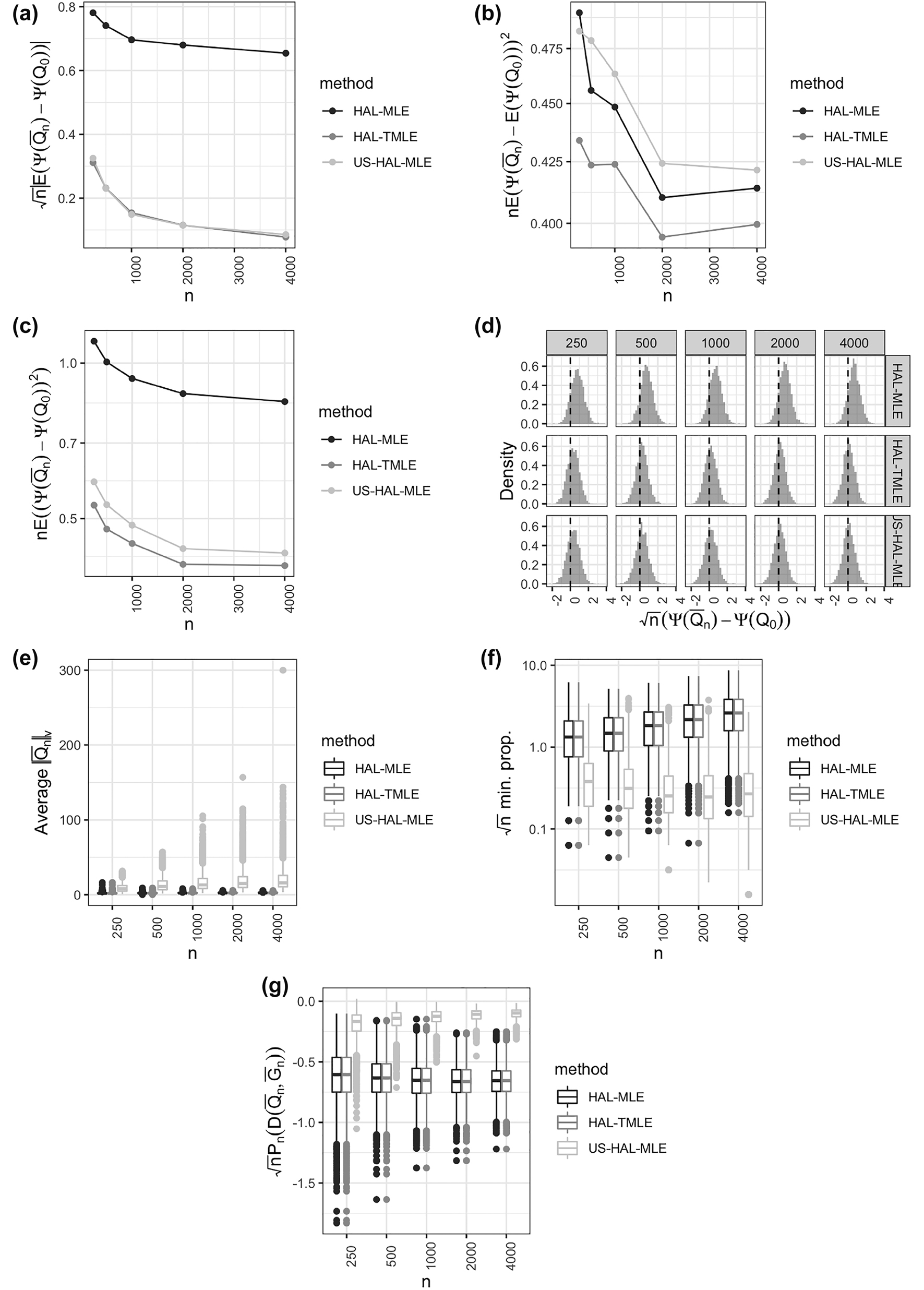
Simulation results for the treatment-specific mean parameter: (a) bias in absolute value, (b) variance, (c) mean-squared error (all scaled by n 1/2), (d) Sampling distribution of scaled and centered estimator, (e) Sectional variation norm of the nuisance parameter, (f) empirical average of quantity given in Eq. (5), (g) sample average of the efficient influence function, evaluated at the sample estimate.
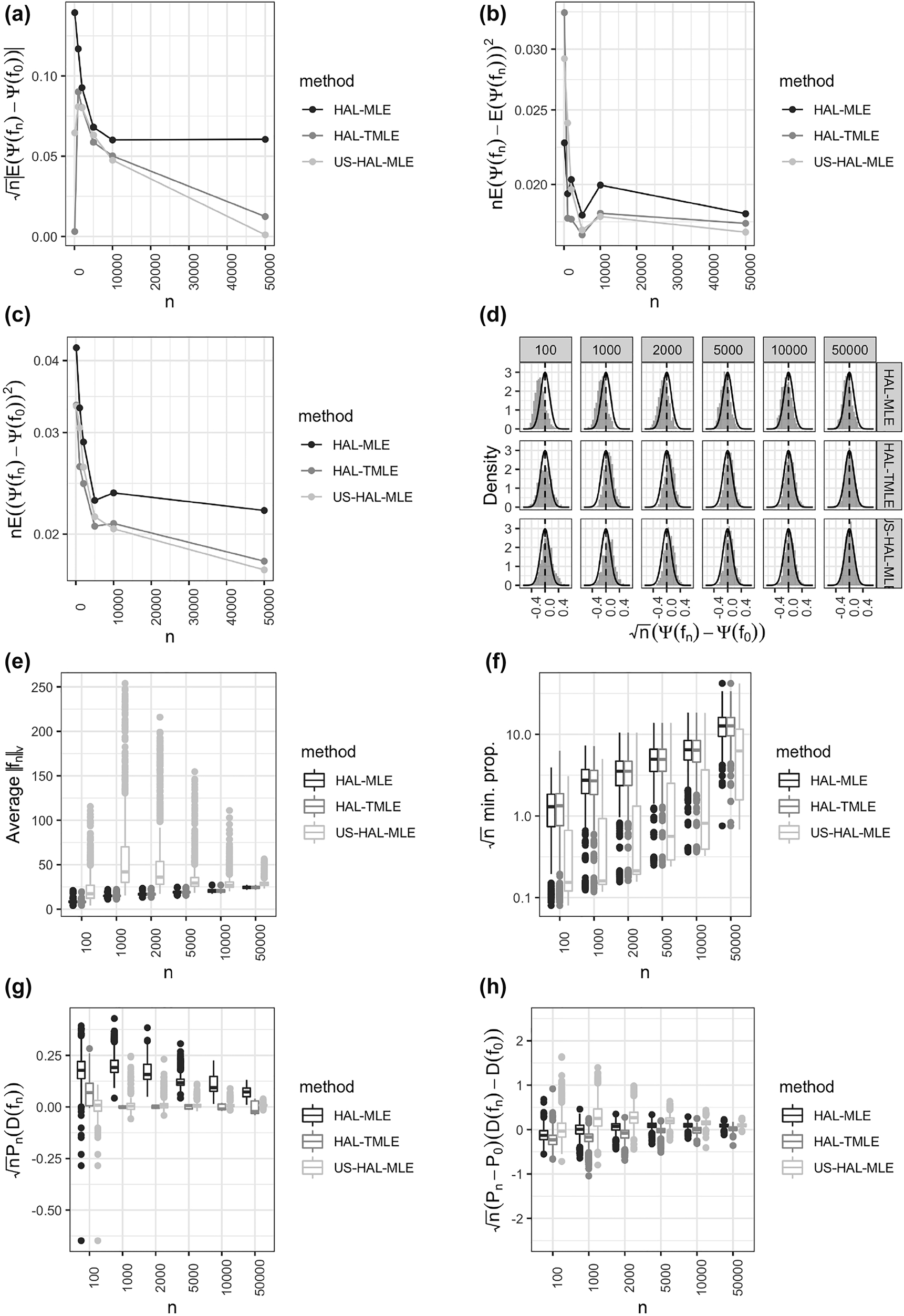
Simulation results for the average density value parameter: (a) bias in absolute value (b) variance (c) mean-squared error (all scaled by n
1/2); (d) Sampling distribution of scaled and centered estimator, (e) Sectional variation norm of the nuisance parameter (f) empirical average of quantity given in Eq. (5), (g) sample average of the efficient influence function, evaluated at the sample estimate, (h)
6.2 Simulations for the integral of the square of the density
We simulated a univariate variable O ∼ N(−4, 5/3) and evaluated the performance of undersmoothed HAL for estimating the integral of the square of the density of O (Section 5). We implemented a HAL-based estimator of the density using an approach similar to the one described in [28]. This approach entails estimating a discrete hazard function using HAL using a pre-specified binning of the real line. For this simulation, we used 320 equidistant bins, and note that the HAL density estimator is robust to this choice, so long as a large enough value is chosen. We sample 1000 data sets for each of several sample sizes ranging from n = 100 to 100,000. We compare the results for undersmoothed HAL to those obtained by using a typical implementation of HAL that selects the level of smoothing based on cross-validation. We compared these estimators on the same criterion described in the previous subsection.
The simulations results reflect what is expected based on theory. In particular, the undersmoothed HAL achieves the efficiency bound in large samples and the scaled-centered sampling distribution of the estimator is well approximated by the efficient asymptotic distribution. We found that our selection criterion for the level of undersmoothing based on the EIF led to control of the variation norm of the resultant fit. On the other hand, results for the HAL estimator with level of smoothing selected via cross-validation demonstrated that this estimator does not have bias that is decreasing faster than n −1/2. Thus, this estimator performs worse in terms of all criteria that we considered. The estimated cross-validated and undersmoothed function paths as well as the true function are illustrated in Figure 3.
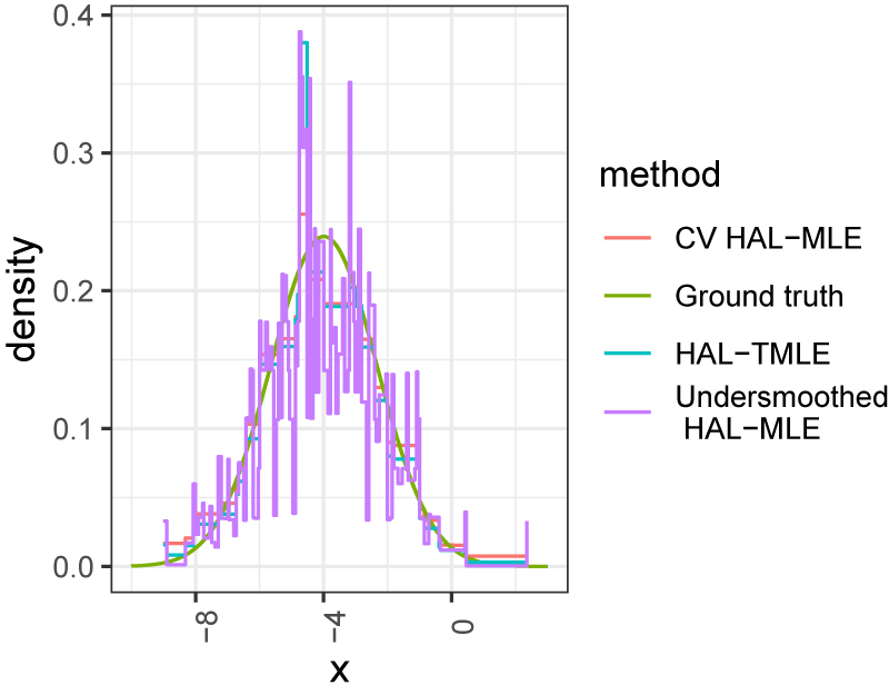
A random realization of the Simulation in Section 7.2 (n = 500).
7 Discussion
In this article we established that for realistic and nonparametric statistical models an overfitted zero-order spline HAL-MLE of a functional parameter of the data distribution results in efficient plug-in estimators of pathwise differentiable functionals of this functional parameter. The statistical model can be any model for which the parameter space of the functional parameter is a (cartesian product of a) subset of the set of multivariate cadlag functions with a universal bound on the sectional variation norm. The undersmoothing condition involves two purposes. Firstly, one wants to undersmooth so that solving the L
1-constrained scores P
n
S
h
(Q
n
) with r(h, Q
n
) = 0 implies solving P
n
S
h
(Q
n
) = o
P
(n
−1/2), and thereby
The undersmoothing conditions presented are not parameter specific, so that such an undersmoothed HAL-MLE will be efficient for any of its smooth functionals. In addition, the undersmoothing of the HAL-MLE does not change its rate of convergence relative to the HAL-MLE optimally tuned with cross-validation, as long as the selected L 1-norm remains uniformly bounded, suggesting that it is still a good estimator of the true functional parameter.
On the other hand, a typical TMLE targeting one particular target parameter will generally only be asymptotically efficient for that particular target parameter, and not even asymtotically linear for other smooth functionals, even if it uses as initial estimator the HAL-MLE tuned with cross-validation. Therefore it appears to be an interesting topic to better understand the sampling distribution of the undersmoothed HAL-MLE in an asymptotic sense and in relation to a sampling distribution of a TMLE using an optimally smoothed (i.e., cross-validation) HAL-MLE as initial estimator. Note, however, that if the TMLE uses an undersmoothed HAL-MLE as initial estimator, than the TMLE step should result in small changes, thereby mostly preserving the behavior of the undersmoothed HAL-MLE. Therefore, the latter type of TMLE might be recommended, inheriting the good global behavior of the HAL-MLE, also in light of the recent work on higher order TMLE [29].
It is also of interest to observe that the second order remainder of the HAL-MLE for a pathwise differentiable functional appears to either be driven by the square of the L 2(P 0)-norm of the HAL-MLE itself with respect to the functional parameter, or, in the case that the efficient influence curve has a nuisance parameter G, a second order remainder might also (or only) involve a product of differences of the HAL-MLE Q n with respect to its true counterpart Q 0 and the difference of a projection G 0,n of the true G 0 with respect to the linear space of basis functions selected by the undersmoothed HAL-MLE Q n . Since G 0,n is a type of oracle estimator of G 0, this suggest that in a model in which our knowledge on G 0 is not any better than our knowledge on Q 0, this HAL-MLE has a good second order remainder that might generally be smaller than what it would be for a TMLE that estimates G 0 with an actual estimator such as the HAL-MLE.
On the other hand, if the statistical model involves particularly strong knowledge on the nuisance parameter G 0, then a TMLE can fully utilize this model on G 0 and thereby obtain a better behaved second order remainder than the one for the overfitted HAL-MLE. One also suspects that a TMLE will be more sensitive to lack of positivity for the target parameter than the undersmoothed HAL-MLE. Therefore, we conjecture that an undersmoothed HAL-MLE might be the preferred estimator in models in which case the estimation of G 0 is as hard as estimation of Q 0, and when lack of positivity is a serious issue, while an HAL-TMLE might be the preferred estimator when estimation of G 0 is easier than estimation of Q 0. These are not formal statements, but indicate a qualitative comparison between the undersmoothed HAL-MLE and a HAL-TMLE using an estimator (HAL-MLE) G n of G 0.
However, this above comparison has an additional twist of interest in favor of the HAL-MLE. That is, if G 0 happens to be a function with relative small variation norm, unknown to the analyst, then we will have much faster convergence of G 0,n to G 0 than if the true G 0 is very complex. As such the undersmoothed HAL-MLE will have a remainder involving a very fast converging G 0,n , possibly faster than the estimator G n used by the TMLE utilizing this simple model. Thus, the HAL-MLE is able to adapt to underlying (unknown) smoothness of G 0, making it even less obvious that TMLE utilizing knowledge on G 0 will do any better. All of this strongly suggest that the TMLE should use an undersmoothed HAL-MLE as initial estimator and make sure that the targeting step does not destroy the score equations already solved by the HAL-MLE. We will address the latter in a future article.
In future research we will address the comparison between undersmoothed HAL-MLE and HAL-TMLE in realistic simulations and by formal comparison by their second order remainders (some of it already shown by [29]). Specifically, in a subsequent article we will marry the TMLE with the HAL-MLE by defining a targeted HAL-MLE that minimizes the empirical risk over the linear span of basis functions (approximating the true cadlag function with finite sectional variation norm) under the L 1-constraint and under the constraint that the Euclidean norm of the empirical mean of the efficient influence curve at the HAL-MLE (as well as at an estimator G n ) is o P (n −1/2). We will show that undersmoothing this targeted HAL-MLE results in an estimator that is still efficient across all smooth functionals, while it is able to fully exploit all knowledge on G 0 for the sake of the specific target parameter. Moving forward it will also be critically important to compare approaches for building confidence intervals and performing hypothesis tests.
A key advantage of a TMLE is that it can utilize any super-learner so that its library can include many other powerful machine learning algorithms, including many variations of the HAL-MLE. In this manner a TMLE using a powerful super-learner might compensate for the favorable property of an undersmoothed HAL-MLE with respect to size of the second order remainder. In another future article we will provide a method that marries a powerful super-learner with HAL-MLE, by using the super-learner as a dimension reduction, and applying HAL-MLE as the meta learning step in an ensemble learner. We will show that an undersmoothed HAL-MLE in this metalearning step will result again in an estimator that is efficient, and possibly super-efficient, for any of its smooth functionals. By actually using a targeted HAL-MLE as meta learning step, we might end up with an estimator that is able to still fully exploit the strengths super-learning, undersmoothed HAL-MLE, and TMLE using a good estimator of G 0, combined in one method.
Undersmoothing of HAL-MLE can also be applied to nuisance parameters such as an HAL-MLE of the censoring and treatment mechanism in an inverse probability of treatment and censoring weighted (IPTCW) estimator. By undersmoothing the HAL-MLE G n of the censoring and treatment mechanism G 0, smooth functionals of G n become asymptotically efficient just as shown in this article for undersmoothed Q n . An analysis of an IPTCW estimator precisely relies on showing that a smooth functional of G n is asymptotically linear. Therefore, in this manner we can show that an IPTCW-estimator that uses an undersmoothed HAL-MLE for estimation of the censoring and treatment mechanism is regular and asymptotically linear and even efficient if the full data model is saturated [30].
Finally, we refer to our accompanying technical report [31] that presents a generalization of this highly adaptive lasso estimator to minimizers of empirical risk over smoothness classes that are spanned by the higher order spline basis functions. The current HAL-MLE corresponds with zero-order spline basis functions. The order of the spline can be selected with cross-validation resulting in an HAL-MLE that also adapts to underlying smoothness. We plan to publish this part in a later article.
Funding source: National Institute of Allergy and Infectious Diseases
Award Identifier / Grant number: 5R01AI074345-09
-
Author contribution: All the authors have accepted responsibility for the entire content of this submitted manuscript and approved submission.
-
Research funding: This work was supported by the National Institute of Allergy and Infectious Diseases (grant number 5R01AI074345-09).
-
Conflict of interest statement: The authors declare no conflicts of interest regarding this article.
Appendix A: Proof of Theorem 1 and Lemma 1
The HAL-MLE has the form
Consider paths (1 + ϵh(j))β n (j) for a bounded vector h, which yields a collection of scores
Let
Thus, by β
n
being an MLE, P
n
S
h
(Q
n
) = 0 for any h satisfying r(h, Q
n
) = 0. Let
This gives
So
where
We note that c
n
(j*) is bounded by ∑
j
∣h*(j)‖β
n
(j)∣. So we can bound this by ∥h*∥∞
C
n
. Thus under the assumption that
For this choice
Therefore, our undersmoothing condition is that
Under this condition we have
Let now
Let
but P
0
S
j
(Q
0) = 0 for all j, since Q
0 = arg min
Q
P
0
L(Q). Therefore,
This proves the second statement of Theorem 1. The third statement is a trivial implication, which completes the proof of Theorem 1. □
Proof of Lemma 1
Consider the special case that O = (Z, X), L(Q)(O) depends on Q through Q(X) only, and
We assume
Then, (16) reduces to
This teaches us that the critical condition (14) holds if
and that for this choice j* we have
Appendix B: Proof of Theorem 2
Let G
0n
be an approximation of G
0, and let D*(Q
n
, G
0n
) be the approximation of D*(Q
n
, G
0) in the space of scores
Theorem 5
Consider the HAL-MLE Q
n
with C = C
u
or C = C
n
. Assume M
1, M
20 < ∞. We have
R 2((Q n , G 0n ), (Q 0, G 0)) = o P (n −1/2) and
Then Ψ(Q n ) is asymptotically efficient at P 0.
Proof
The exact second order expansion at G 0n of the target parameter Ψ yields
Given that
□
This theorem can be easily generalized to a more general approximation
Theorem 6
Consider the HAL-MLE Q
n
with C = C
u
or C = C
n
. Assume M
1, M
20 < ∞. We have
R 2((Q n , G 0), (Q 0, G 0)) = o P (n −1/2),
Then Ψ(Q n ) is asymptotically efficient at P 0.
Therefore, in order to prove Theorem 2, it remains to establish the condition under which (17) holds, which was proven in the previous Appendix A.
B.1 General proof of efficient score equation condition at G 0
This subsection can be skipped for the purpose of proving Theorem 2, but the following result fits here.
Lemma 3
Under the conditions of Theorem 5, if P
n
D*(Q
n
, G
0n
) = o
P
(n
−1/2), then also P
n
D*(Q
n
, G
0) = o
P
(n
−1/2). Under the conditions of Theorem 6, if
Proof
Firstly, we have
In addition, we have
since
To understand the last term, consider the case that
In our general Theorem 5 we assumed R 20(Q n , G 0n , Q 0, G 0) = o P (n −1/2), which certainly implies R 20(Q n , G 0, Q 0, G 0) (which actually equals zero in double robust problems). This then establishes that
For general
References
1. Bickel, PJ, Klaassen, CAJ, Ritov, Y, Wellner, J. Efficient and adaptive estimation for semiparametric models. Berlin, Heidelberg, New York: Springer; 1997.Search in Google Scholar
2. Newey, W. The asymptotic variance of semiparametric estimators. Econometrica 2014;62:1349–82.10.2307/2951752Search in Google Scholar
3. van der Laan, MJ. Causal effect models for intention to treat and realistic individualized treatment rules. In: Technical report 203. Berkeley: Division of Biostatistics, University of California; 2006.10.2202/1557-4679.1022Search in Google Scholar PubMed PubMed Central
4. van der Vaart, AW. Asymptotic statistics. Cambridge, New York; 1998.10.1017/CBO9780511802256Search in Google Scholar
5. Shen, X. On methods of sieves and penalization. Annals of Statitics 1997;252:2555–91. https://doi.org/10.1214/aos/1030741085.Search in Google Scholar
6. Shen, X. Large sample sieve estimation of semiparametric models. In: Chapter in handbook of econometrics, vol 76; 2007.10.1016/S1573-4412(07)06076-XSearch in Google Scholar
7. Giné, E, Nickl, R. A simple adaptive estimator of the integrated square of a density. Bernoulli 2008;14:47–61. https://doi.org/10.3150/07-bej110.Search in Google Scholar
8. Hahn, J. On the role of the propensity score in efficient semiparametric estimation of average treatment effects. Econometrica 1998;2:315–31. https://doi.org/10.2307/2998560.Search in Google Scholar
9. Newey, WK, Robins, JR. Cross-fitting and fast remainder rates for semiparametric estimation. arXiv preprint arXiv:1801.09138 2018.10.1920/wp.cem.2017.4117Search in Google Scholar
10. Newey, WK, Hsieh, F, Robins, JM. Twicing kernels and a small bias property of semiparametric estimators. Econometrica 2004;72:947–62. https://doi.org/10.1111/j.1468-0262.2004.00518.x.Search in Google Scholar
11. Robins, JM, Rotnitzky, A. Recovery of information and adjustment for dependent censoring using surrogate markers. In: AIDS epidemiology. Basel: Birkhäuser; 1992.10.1007/978-1-4757-1229-2_14Search in Google Scholar
12. van der Laan, MJ, Robins, JM. Unified methods for censored longitudinal data and causality. Berlin, Heidelberg, New York: Springer; 2003.10.1007/978-0-387-21700-0Search in Google Scholar
13. van der Laan, MJ. Estimation based on case-control designs with known prevalance probability. Int J Biostat 2008;4:17. https://doi.org/10.2202/1557-4679.1114.Search in Google Scholar PubMed
14. van der Laan, MJ, Gruber, S. One-step targeted minimum loss-based estimation based on universal least favorable one-dimensional submodels. Int J Biostat 2016;12:351–78. https://doi.org/10.1515/ijb-2015-0054.Search in Google Scholar PubMed PubMed Central
15. van der Laan, MJ, Rose, S. Targeted learning: causal inference for observational and experimental data. Berlin, Heidelberg, New York: Springer; 2011.10.1007/978-1-4419-9782-1Search in Google Scholar
16. van der Laan, MJ, Rubin, DB. Targeted maximum likelihood learning. Int J Biostat 2006;2:11.10.2202/1557-4679.1043Search in Google Scholar
17. Benkeser, D, van der Laan, MJ. The highly adaptive lasso estimator. In: 2016 IEEE international conference on data science and advanced analytics (DSAA). Montreal, QC, Canada: IEEE; 2016:689–96 pp.10.1109/DSAA.2016.93Search in Google Scholar PubMed PubMed Central
18. van der Laan, MJ. A generally efficient targeted minimum loss-based estimator. In: Technical report 300. UC Berkeley; 2015. to appear in IJB, 2017 http://biostats.bepress.com/ucbbiostat/paper343.10.1515/ijb-2015-0097Search in Google Scholar PubMed PubMed Central
19. Gill, RD, van der Laan, MJ, Wellner, JA. Inefficient estimators of the bivariate survival function for three models. Ann Inst Henri Poincaré 1995;31:545–97.Search in Google Scholar
20. Polley, EC, Rose, S, van der Laan, MJ. Super learner. In: van der Laan, MJ, Rose, S, editors. Targeted learning: causal inference for observational and experimental data. New York, Dordrecht, Heidelberg, London: Springer; 2011.10.1007/978-1-4419-9782-1_3Search in Google Scholar
21. van der Laan, MJ, Dudoit, S. Unified cross-validation methodology for selection among estimators and a general cross-validated adaptive epsilon-net estimator: finite sample oracle inequalities and examples. In: Technical report 130. Berkeley: Division of Biostatistics, University of California; 2003.Search in Google Scholar
22. van der Laan, MJ, Dudoit, S, van der Vaart, AW. The cross-validated adaptive epsilon-net estimator. Stat Decis 2006;24:373–95.10.1524/stnd.2006.24.3.373Search in Google Scholar
23. van der Laan, MJ, Polley, EC, Hubbard, AE. Super learner. Stat Appl Genet Mol 2007;6:25.10.2202/1544-6115.1309Search in Google Scholar PubMed
24. van der Vaart, AW, Dudoit, S, van der Laan, MJ. Oracle inequalities for multi-fold cross-validation. Stat Decis 2006;24:351–71. https://doi.org/10.1524/stnd.2006.24.3.351.Search in Google Scholar
25. Bibaut, A, van der Laan, MJ. Fast rates for empirical risk minimization over cadlag functions with bounded sectional variation norm. In: Technical report. Berkeley: Division of Biostatistics, University of California; 2019.Search in Google Scholar
26. van der Laan, MJ, Bibaut, A. Uniform consistency of the highly adaptive lasso of infinite dimensional parameters. In: Technical report arXiv:1709.06256. Berkeley: Division of Biostatistics, University of California; 2017.Search in Google Scholar
27. Cai, W, van der Laan, MJ. Nonparametric bootstrap inference for the targeted highly adaptive least absolute shrinkage and selection operator (lasso) estimator. Int J Biostat 2020;16:20170070. https://doi.org/10.1515/ijb-2017-0070.Search in Google Scholar PubMed
28. Diaz Munoz, I, van der Laan, MJ. Super learner based conditional density estimation with application to marginal structural models. Int J Biostat 2011;7:1–20. https://doi.org/10.2202/1557-4679.1356.Search in Google Scholar PubMed
29. van der Laan, MJ, Wang, Z, van der Laan, LWP. Higher order targeted maximum likelihood estimation; 2021.Search in Google Scholar
30. Ertefaie, A, Hejazi, NS, van der Laan, MJ. Nonparametric inverse probability weighted estimators based on the highly adaptive lasso; 2020.Search in Google Scholar
31. van der Laan, MJ, Benkeser, D, Cai, W. Efficient estimation of pathwise differentiable target parameters with the undersmoothed highly adaptive lasso; 2019.Search in Google Scholar
© 2022 Walter de Gruyter GmbH, Berlin/Boston
Articles in the same Issue
- Frontmatter
- Research Articles
- Two-sample t α -test for testing hypotheses in small-sample experiments
- Estimating risk and rate ratio in rare events meta-analysis with the Mantel–Haenszel estimator and assessing heterogeneity
- Estimating population-averaged hazard ratios in the presence of unmeasured confounding
- Commentary
- Comments on ‘A weighting analogue to pair matching in propensity score analysis’ by L. Li and T. Greene
- Research Articles
- Variable selection for bivariate interval-censored failure time data under linear transformation models
- A quantile regression estimator for interval-censored data
- Modeling sign concordance of quantile regression residuals with multiple outcomes
- Robust statistical boosting with quantile-based adaptive loss functions
- A varying-coefficient partially linear transformation model for length-biased data with an application to HIV vaccine studies
- Application of the patient-reported outcomes continual reassessment method to a phase I study of radiotherapy in endometrial cancer
- Borrowing historical information for non-inferiority trials on Covid-19 vaccines
- Multivariate small area modelling of undernutrition prevalence among under-five children in Bangladesh
- The optimal dynamic treatment rule superlearner: considerations, performance, and application to criminal justice interventions
- Estimators for the value of the optimal dynamic treatment rule with application to criminal justice interventions
- Efficient estimation of pathwise differentiable target parameters with the undersmoothed highly adaptive lasso