Maximum Likelihood Estimation in a Semicontinuous Survival Model with Covariates Subject to Detection Limits

1 Introduction

Semicontinuous data are common in medical and biological studies and typically occur when there is a point mass at zero and a continuous, right-skewed distribution over a positive range. Researchers have analyzed this type of data in a variety of applications, including annual medical expenses [1, 2], daily alcohol intake [3], driving scores [4], and health assessment scores [5]. Manning et al. [6], Duan et al. [7], Moulton et al. [8] and Olsen and Schafer [9], among many others, have suggested two-part mixture models for handling both cross-sectional and longitudinal semicontinuous data. In the presence of covariates, the two-part model usually employs logistic regression to model the probability of observing a zero outcome and a continuous regression model to describe the distribution of outcomes above zero.

In the motivating Genetic and Inflammatory Markers of Sepsis (GenIMS) Study, biological measurements were collected on patients admitted to the hospital with community acquired pneumonia (CAP). One of the main purposes of the study was to determine how three cytokine biomarkers are related to survival for patients with CAP. Unlike typical analyses of time-to-event data, the original study investigators were primarily interested in modeling the binary event of surviving at least 90 days [10], based on recommendations by two international expert panels, which suggested that most if not all deaths due to pneumonia and resulting sepsis would have occurred by this time [11, 12]. Alternatively, some recent analyses of the data have directly modeled the available survival times [e.g., [13, 14, 15].

Rather than choosing between a binary and continuous survival outcome, we suggest simultaneously modeling the event of surviving 90 days and the actual survival times for those not surviving to 90 days. In order to frame this problem in a familiar way, we note that for the purposes of the GenIMS study, we may conceptually consider the patients who survived to 90 days as cured from CAP. Though cure rate models have been developed to model long-term survival data [16, 17], a typical cure rate model does not apply for the GenIMS data set since the cure status is known for all individuals and the survival part of the model is truncated. Thus, we instead suggest framing the problem in the context of a semicontinuous regression model, which in this survival modeling context we term a semicontinuous survival model. Unlike in a typical semicontinuous data model, the continuous part of the distribution occurs between zero and 90, while the point mass occurs at 90.

An additional complication with the GenIMS data set is that the biomarker covariates of interest are subject to lower detection limits (DLs). Traditionally, a few common approaches have been taken to handle censoring due to DLs. One approach has been to replace the censored observations using either a function of the DL, such as DL/2 [see [18], or the conditional mean of the censored covariate [19, 20]. These naive substitution methods have been shown to lead to biased parameter estimates in generalized linear models [21, 22, 23, 24, 25, 26, 27] and survival models [13, 14, 15]. An alternative approach only uses complete cases. While this strategy still leads to unbiased parameter estimates as long as censoring is only caused by the DL, efficiency is lost due to the discarding of data.

Several authors have considered more sophisticated approaches to handling DLs in the context of survival data. Langohr et al. [28] and Sattar et al. [15] proposed fully-parametric survival models with an interval-censored predictor while Bernhardt et al. [13] used multiple imputation techniques for accelerated failure time models with left-censored covariates. In the context of semiparametric Cox proportional hazards models with covariates subject to DLs, Lee et al. [29] suggested a partial likelihood approach based on an empirical estimate of the relative risk function using uncensored covariate observations, D’ Angelo and Weissfeld [14] developed an indexing approach where censored covariate values are directly replaced by their conditional expectation given a linear combination of the fully observed covariates, and Chen et al. [30] considered a Bayesian strategy where the censored covariates are modeled parametrically. Recently, [31] suggested using a nonparametric density estimator for a single censored covariate in the context of frailty models.

All of the methods mentioned above for handling covariates subject to DLs in survival models are either statistically naive — such as the DL/2 and complete case methods — or do not consider a model set-up where individuals are no longer considered to experience the event of interest after a fixed time point. In the context of semicontinuous models, which we propose to model this special type of data, the issue of covariates subject to DLs has not been previously considered. Additionally, to our knowledge, prior statistical analyses using semicontinuous regression models have not included a case where the continuous portion of the distribution is bounded above.

In this paper, we propose a straightforward and flexible method for analyzing a semicontinuous survival outcome with covariates subject to DLs, where the interest lies in estimating both the associations of covariates with the survival time for those experiencing the event of interest and the associations of covariates with the probability of surviving to the known “cure time.” We suggest using a truncated accelerated failure time model to model the survival times for those experiencing the event of interest and a logistic regression to model the probability of being cured (surviving to the “cure time”). We propose using a series of mixture of normal regression models to flexibly model the multivariate distribution of the censored covariates, though our modeling strategy allows for a more standard parametric model or even a semiparametric approach. To obtain estimates in this semicontinuous survival model, we develop a Monte Carlo EM algorithm where to estimate the expectation in the E-step, multiple imputations are generated for the censored covariates according to a mixture of normals distribution, and weighted maximum likelihood is applied to the observed and imputed data.

The remainder of the paper is organized as follows. In Section 2, we develop our proposed semicontinuous survival model, including our proposal for the distribution of the covariates. In Section 3, we present a Monte Carlo EM algorithm for obtaining parameter estimates. In Section 4, we summarize the main goals of inference as well as some notes on model checking. In Section 5, we conduct a simulation study comparing our proposed method to naive or less flexible methods. In Section 6, we apply our method to the GenIMS data set. Finally, in Section 7, we briefly review our method and discuss its advantages and shortcomings.

2 Semicontinuous survival model

3 Monte carlo EM algorithm

Unless q is small, eq. (2) may be extremely challenging to maximize directly using algorithms like the Newton-Raphson method, since a potentially high-dimensional integral would need to be evaluated for each individual at each iteration in the maximization procedure. Thus, in order to maximize the likelihood eq. (2), we suggest using an expectation-maximization (EM) algorithm, originally described by [35]. The main advantages of using the EM algorithm for maximization over competing methods are that it is very numerically stable [36] and is convenient in the presence of missing data. Maximization is achieved by iterating between two steps, the E-step and M-step. In the E-step, the expected value of the log-likelihood of the complete data is calculated with respect to the missing data conditional on all of the observed data at a set of current parameter estimates. In the M-step, this expected log-likelihood is maximized to obtain new parameter estimates. In this section, we extend the EM algorithm to handle covariates subject to DLs in the context of a semicontinuous survival model.

Suppose that, without loss of generality, we observe δi=1 for the first r individuals and δij=0 for at least one covariate Xij for the remaining n−r individuals. In the E-step of the EM algorithm, the conditional expected value of the log-likelihood with respect to the missing data can be represented by

A closed form expression of eq. (5) is usually not attainable, so we propose a Monte Carlo approach for estimating this integral, originally suggested by Wei and Tanner [37], in the same spirit as Ibrahim [34] for missing data in parametric regression models and May et al. [38] for generalized linear models with covariates subject to censoring. Specifically, we estimate Qi∗(θ|θ(t)) as

where xil, l=1,⋯,m, are randomly sampled from fiT(xicen|yi,xiobs,zi;θ(t)), the distribution of Xicen|Yi,Xiobs,Zi truncated above at di. Standard Monte Carlo sampling techniques can be used to obtain samples from this distribution by noting that

In practice, we use a random walk Metropolis method [39] with truncated Gaussian proposals.

For the M-step of the EM algorithm, we then maximize eq. (5) with the Monte Carlo estimate eq. (6) replacing Qi∗, i=r+1,⋯,n. This maximization can be done in three separate parts: a maximization for the part involving the parameters in the logistic regression,

a maximization for the part involving the parameters in the distribution of the time-to-event variable for those experiencing an event,

and a maximization for the part involving the parameters in the distribution of the covariates subject to DLs,

The eqs. (7) and (8) can be maximized using standard optimization routines for logistic regression and AFT models, respectively, for a set of r+(n−r)m complete observations, where each of the (n−r)m parts involving the imputed xil values is given weight 1/m. If a series of mixture of normal regressions is used to model the distribution f(xi|zi), we can similarly conduct a series of weighted maximizations for eq. (9) using an EM algorithm for mixture distributions (e.g., [40]). The E and M steps are then iterated until the parameter estimates converge.

We summarize the steps for the proposed Monte Carlo EM algorithm, with additional details and computational tips based on the statistical software R.

1. Obtain initial values for estimating the parameters {β,η,γ}, {βˆ(1),ηˆ(1),γˆ(1)}, by maximizing eq. (2) for the complete cases. The “optim’ function can be used to obtain estimates for β and η in the truncated AFT model while the function “glm” can be used to obtain estimates for γ in the logistic regression model. Obtain initial estimates for the parameters {π,α,τ}, {πˆ(1),αˆ(1),τˆ(1)}, by maximizing eq. (3) with censored Xij values replaced by random draws from a normal distribution truncated above at dij. The function “flexmix” in the flexmix package [41] can be used to obtain these estimates.

2. At the (t+1)th step of the EM algorithm, given the current set of parameter estimates θˆ(t), generate m imputed vectors for each Xicen. The function “metrop” in the mcmc package [42] can be used to efficiently obtain samples.

3. Update θˆ(t) as θˆ(t+1) by maximizing eqs. (7), (8), and (9). The functions flexsurvreg, glm, and flexmix can all handle weighted observations for obtaining maximum likelihood estimates.

4. Repeat steps 2-3 until

   max|θˆ1(t+1)−θˆ1(t)||θˆ1(t)|,⋯,|θˆs(t+1)−θˆs(t)||θˆs(t)|<ϵ,

   where s is the number of elements in θ and ε is a predefined distance. Define the maximum likelihood parameter estimate as θˆ=θˆ(t+1).

In practice, we recommend letting m, the number of Monte Carlo imputations for Xicen, depend on the iteration t by starting with a relatively small m, say 5-15, and increasing m gradually. To obtain variance estimates for θˆ, the method of Louis [43] can be used to estimate the observed information matrix. Alternatively, if it is computationally feasible, standard software can be used to calculate the Hessian matrix for the observed data likelihood eq. (2) at the final set of parameter estimates or bootstrapping can be conducted on the original data set. Finally, we note that the imputations for Xicen could be obtained in semiparametric or nonparametric manner rather than using a mixture of normal regressions. However, we feel that a parametric approach often takes the most advantage of the data information above the DL in order to extrapolate imputations below the DL.

4 Inference and model checking

Recall that the main analysis goals in the semicontinuous survival regression model are to estimate β and γ, the parameters relating the covariates to the continuous and discrete components of the response, and to determine significance of the associations between the covariates and the semicontinuous survival variable.

While estimating β and γ as described in Section 3 is relatively complicated, interpreting βˆ and γˆ is straightforward. Since the binary and continuous parts of the survival model do not share parameters, they can be considered separately (simultaneous maximization is only required due to the censoring on the covariates). Then, in the logistic regression submodel, exp{γj}, j=1,⋯,p+1, represent the multiplicative changes in odds of surviving to time c, while in the AFT submodel, exp{βj}, j=1,⋯,p+1, represent the multiplicative changes in survival times for those experiencing the event of interest before time c.

To assess whether the jth covariate is associated with the survival outcome, the hypothesis test of interest is H0:βj=γj=0 versus Ha:βj≠0 or γj≠0. Since the proposed model is entirely parametric, it is reasonable to calculate the likelihood ratio statistic −2log{LH0(θˆ)/LHa(θˆ)} and compare it to the (1−α)th quantile of a chi-squared distribution with 2 degrees of freedom.

With the proposed parametric modeling scheme, it is important to choose a good model prior to conducting inference. In practice, we suggest fitting several competing models and comparing them using standard tools for assessing fit such as AIC or BIC. For modeling the binary event of surviving to time c, two popular choices are probit and logistic regression, while for modeling the observed survival times less than c, lognormal, exponential, Weibull, gamma, and generalized gamma models, among others, could be considered. Even if these response models are reasonable, a poor imputation model for the censored covariates could bias inference. While we suggested a flexible mixture of normal regressions approach, alternative distributions could be considered. However, we show in Section 5 that the mixture of normals performs well in a variety of scenarios.

After choosing the best model among those considered, residual analyses or goodness-of-fit tests may be of interest to further confirm that the best model is in fact a reasonable model. However, diagnostics are complicated by the censoring on X. One obvious choice for constructing residuals or fitted responses in this scenario is to simply replace the censored values of a covariate by the average of the m values generated at the last iteration of the Monte Carlo EM algorithm. Alternatively, as suggested by [44] and [45], these m imputations could be used to form m multiply imputed data sets after which usual model validation techniques can be conducted repeatedly and summarized appropriately.

5 Simulation study

We conducted simulations to study the performance of our proposed semicontinuous survival model. We set up the simulations to represent a situation similar to that in the GenIMS application described in Section 6, and we compared the proposed method to other practical approaches.

5.1 Single censored covariate: response model known

We generated N = 500 data sets of size n = 200 with a survival response Yi, a single covariate Xi subject to a DL, and a vector of fully observed covariates Zi. Specifically, we generated the covariates Zi1∼iidbeta(3,2)⋅84+18, to represent an “age” variable, and Zi2∼iidBernoulli(0.49), to represent a gender variable with P(male) = 0.49. We also generated a continuous covariate Zi3|Zi1,Zi2∼ind.N(μi=30+5Zi1+0.4Zi2,σ2=20). For the first set of simulations, we let Xi|Zi∼ind.pN(μi=(1,Zi1,Zi2,Zi3)α1,σ2=1)+(1−p)N(μi=(1,Zi1,Zi2,Zi3)α2,σ2=1) where p∼iidBernoulli(0.3) and α=(α1T,α2T)T=(5,−0.03,1,0.05,2,0.08,1,−0.1)T. Values for the DL d, which we did not vary across individuals, were chosen so as to produce either 20% or 40% censoring on the covariate Xi.

The values for α were chosen so that the distribution of Xi|Zi is clearly non-normal for many values of Zi but the marginal distribution of Xi appears plausibly normal. Figure 1 shows a histogram, estimated density, and normal probability plot for 10,000 random samples from the distribution of Xi when there is no censoring as well as a histogram for 10,000 random samples from the distribution Xi|Zi for a randomly generated Zi. While the marginal distribution of Xi appears reasonably normal, assuming normality for the conditional distribution of Xi would not be reasonable. We chose this set-up to demonstrate that it may be wise to choose a flexible distribution for Xi|Zi even if the covariate appears to be marginally distributed according to a normal or another well-known density.

Figure 1:

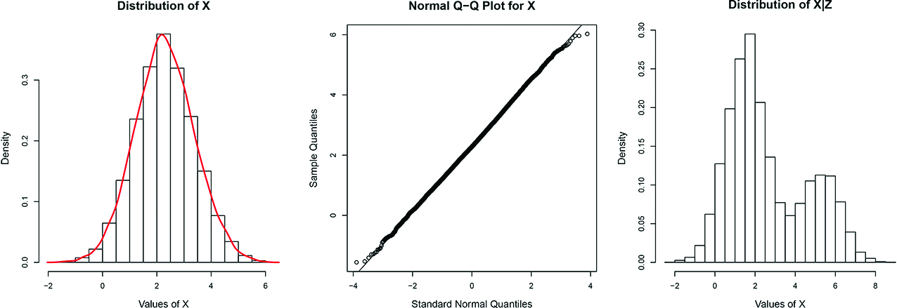
From left to right: (1) Histogram and estimated density for X based on 10,000 randoms samples; (2) Normal q-q plot based on same 10,000 random samples; (3) Histogram for X conditional on a single randomly generated Z based on 10,000 random samples.

We generated the log of the survival response as log(Yi)|Xi,Zi∼ind.TN+log(90)(μi=(1,Xi,ZiT)β,σ2=4), where β=(2,1,−0.01,−1,−0.05)T and TN+log(90) represents a normal distribution truncated above at log(90) since 90 days is the threshold in the GenIMS study. Finally, we let Yi=90 with probability [1+exp{(1,Xi,ZiT)γ}]−1, where γ=(−1,0.7,−0.05,−1,0.03)T so that about 35% of individuals were cured (i.e. Yi=90).

For the simulations in this section, we assumed that the distributional forms of the semicontinuous survival response were known in order to focus on assessing the proposed Monte Carlo EM estimation approach and the use of a mixture of normals to model the covariate subject to censoring. Specifically, we assumed it was known that a truncated normal AFT model describes the distribution of the log event times for those experiencing an event and a logistic regression describes the probability of never experiencing an event (surviving to 90 days). In Section 5.2, we study simulations for alternative time-to-event and binary regression scenarios.

We considered six data analysis approaches: our proposed semicontinuous survival method using a mixture of two normals for the distribution of Xi|Zi (SS-MN), our proposed semicontinuous survival method using a normal to model the distribution of Xi|Zi (SS-N), a multiple imputation method where 100 imputed data sets were generated assuming the semicontinuous survival model and a normal distribution to model Xi|Zi (MI), an AFT and logistic regression model based on complete data where censored Xi values are replaced with DL/2 (DL), an AFT and logistic regression model using only complete cases (CC), and an AFT and logistic regression model based on the omniscient knowledge of the uncensored covariate values (Omni).

For the MI approach, we used an improper imputation strategy based on fixed parameter estimates to generate imputations from f(Xi|Yi,Zi;θ)∝f(Yi|Xi,Zi;β,η,γ)f(Xi|Yi,Zi;θx). Specifically, we used the complete case estimates for β, η, and γ and maximum likelihood estimates for θx based on a censored normal model. Since these fixed estimates are consistent, the multiple imputation estimates will be asymptotically unbiased [46]. We included the multiple imputation estimator in the simulations for the purpose of comparison, though we do not believe it is an advantageous alternative to our proposed maximum likelihood approach for two reasons. First, obtaining imputations in a truncated region is not standard with current software and usual imputation strategies often do not work well with restricted ranges; thus, it is not computationally simpler. Second, it can be shown that this improper multiple imputation strategy is equivalent to a single iteration in an EM algorithm strategy for maximum likelihood [46, 47], which is the proposed approach.

Table 1:

Single censored covariate: comparison of relative bias and standard deviations (in parenthesis below bias) of estimates for (a) the proposed semicontinuous survival model strategy assuming a mixture of normals distribution for the censored covariate (SS-MN) or a normal distribution for the censored covariate (SS-N); (b) the semicontinuous survival model using multiple imputations based on a normal distribution for the censored covariate (MI); (c) an AFT and logistic regression model replacing censored values with DL/2 (DL); (d) an AFT and logistic regression model using only complete cases (CC); (e) an AFT and logistic regression model based on omniscient knowledge of the uncensored covariate data (Omni). Three underlying distributions for X|Z are considered: a mixture of normals (Mixture), a normal distribution, and log-gamma. Estimates that are biased at the 0.05 level (without multiplicity corrections) are in bold.

Cens.	X|Z	Method	β0	β1	β2	β3	β4	γ0	γ1	γ2	γ3	γ4
20%	Mixture	SS-MN	−0.01	−0.01	−0.03	0.01	0.00	0.03	0.05	0.03	0.07	0.08
			(1.13)	(0.19)	(0.01)	(0.43)	(0.01)	(1.13)	(0.17)	(0.02)	(0.50)	(0.01)
		SS-N	−0.02	0.00	−0.04	0.01	0.00	0.04	0.07	0.03	0.07	0.08
			(1.13)	(0.19)	(0.01)	(0.43)	(0.01)	(1.13)	(0.18)	(0.02)	(0.50)	(0.01)
		MI	−0.02	0.00	−0.04	0.01	0.00	0.04	0.07	0.03	0.07	0.08
			(1.14)	(0.19)	(0.01)	(0.43)	(0.01)	(1.13)	(0.18)	(0.02)	(0.50)	(0.01)
		DL	−0.04	0.01	−0.03	0.01	0.00	0.05	0.08	0.02	0.06	0.07
			(1.14)	(0.19)	(0.01)	(0.43)	(0.01)	(1.13)	(0.18)	(0.02)	(0.50)	(0.01)
		CC	0.00	−0.01	−0.02	0.00	−0.01	0.02	0.05	0.03	0.09	0.07
			(1.17)	(0.20)	(0.01)	(0.44)	(0.01)	(1.20)	(0.20)	(0.02)	(0.52)	(0.01)
		Omni	−0.01	−0.01	−0.03	0.01	−0.01	0.02	0.04	0.03	0.08	0.07
			(1.13)	(0.19)	(0.01)	(0.43)	(0.01)	(1.13)	(0.17)	(0.02)	(0.50)	(0.01)
40%	Mixture	SS-MN	0.02	−0.01	0.10	−0.03	−0.02	0.06	0.08	0.02	0.03	0.01
			(1.39)	(0.13)	(0.02)	(0.50)	(0.01)	(1.19)	(0.15)	(0.02)	(0.51)	(0.02)
		SS-N	0.08	−0.05	−0.15	−0.05	0.03	−0.03	−0.01	0.25	0.14	0.47
			(1.39)	(0.13)	(0.02)	(0.50)	(0.01)	(1.21)	(0.12)	(0.02)	(0.52)	(0.02)
		MI	0.06	−0.03	−0.15	−0.05	0.04	0.01	0.03	0.24	0.16	0.40
			(1.42)	(0.14)	(0.02)	(0.50)	(0.01)	(1.31)	(0.15)	(0.02)	(0.60)	(0.02)
		DL	−0.06	0.08	−0.42	−0.04	0.19	0.19	0.24	0.38	0.21	0.79
			(1.44)	(0.15)	(0.02)	(0.52)	(0.02)	(1.17)	(0.15)	(0.02)	(0.48)	(0.02)
		CC	0.04	−0.01	0.15	−0.02	−0.03	0.14	0.17	0.09	0.28	0.10
			(1.74)	(0.21)	(0.02)	(0.59)	(0.02)	(2.17)	(0.31)	(0.03)	(1.76)	(0.03)
		Omni	0.02	−0.01	0.10	−0.02	−0.02	0.06	0.08	0.03	0.02	0.02
			(1.34)	(0.13)	(0.02)	(0.49)	(0.01)	(1.16)	(0.14)	(0.02)	(0.49)	(0.02)
40%	Normal	SS-MN	−0.05	0.01	−0.01	−0.01	−0.02	0.05	0.05	0.03	0.05	0.03
			(1.17)	(0.16)	(0.01)	(0.46)	(0.01)	(1.02)	(0.15)	(0.01)	(0.41)	(0.01)
		SS-N	−0.05	0.00	−0.02	−0.02	−0.02	0.05	0.05	0.04	0.05	0.05
			(1.17)	(0.16)	(0.01)	(0.46)	(0.01)	(1.01)	(0.15)	(0.01)	(0.41)	(0.01)
		MI	−0.07	0.01	−0.03	−0.01	−0.01	0.06	0.07	0.06	0.05	0.07
			(1.20)	(0.16)	(0.01)	(0.46)	(0.01)	(1.06)	(0.16)	(0.02)	(0.42)	(0.01)
		DL	−0.20	0.10	0.53	−0.03	−0.10	0.24	0.20	−0.11	0.10	−0.25
			(1.22)	(0.18)	(0.01)	(0.47)	(0.01)	(0.98)	(0.17)	(0.01)	(0.38)	(0.01)
		CC	−0.06	0.01	−0.01	0.00	−0.02	0.11	0.10	0.09	0.09	0.09
			(1.56)	(0.23)	(0.02)	(0.54)	(0.02)	(1.62)	(0.25)	(0.02)	(0.60)	(0.02)
		Omni	−0.04	0.00	−0.00	−0.02	−0.02	0.03	0.04	0.04	0.04	0.04
			(1.14)	(0.15)	(0.01)	(0.46)	(0.01)	(0.93)	(0.12)	(0.01)	(0.40)	(0.01)
40%	LogGam	SS-MN	−0.07	0.03	−0.01	0.00	0.00	0.07	0.07	0.00	0.05	−0.03
			(1.18)	(0.24)	(0.02)	(0.46)	(0.02)	(1.02)	(0.20)	(0.02)	(0.37)	(0.01)
		SS-N	−0.08	0.07	−0.24	0.06	0.07	0.10	0.17	0.08	−0.02	0.18
			(1.19)	(0.24)	(0.02)	(0.46)	(0.02)	(1.00)	(0.21)	(0.01)	(0.37)	(0.01)
		MI	−0.08	0.07	−0.20	0.06	0.07	0.11	0.17	0.07	−0.01	0.16
			(1.22)	(0.25)	(0.02)	(0.46)	(0.02)	(1.03)	(0.23)	(0.02)	(0.38)	(0.01)
		DL	−0.12	0.02	0.42	−0.09	−0.11	0.17	0.11	−0.09	0.13	−0.24
			(1.21)	(0.24)	(0.02)	(0.46)	(0.01)	(0.97)	(0.20)	(0.01)	(0.35)	(0.01)
		CC	−0.02	0.00	−0.05	0.00	0.01	0.08	0.08	0.08	0.13	0.08
			(1.56)	(0.34)	(0.02)	(0.55)	(0.02)	(1.68)	(0.38)	(0.02)	(0.56)	(0.02)
		Omni	−0.04	0.00	−0.11	−0.03	0.01	0.05	0.05	0.04	0.08	0.05
			(1.10)	(0.20)	(0.01)	(0.43)	(0.01)	(0.94)	(0.15)	(0.01)	(0.36)	(0.01)

Table 1 displays the relative bias and standard deviation (in parentheses) of the parameter estimates for each of the six analysis methods. The relative bias for a parameter θ is estimated as

θˆ−θ0θ0,

where θˆ=∑j=1Nθˆj/N, θˆj is the parameter estimate for the jth simulated data set, and θ0 is the true parameter value. The standard deviations of the parameter estimator is estimated as

∑j=1N(θˆj−θˆ)2N−1.

Relative biases that are statistically significant at the 0.05 level, without multiplicity corrections, are shown in bold. The first two sections in Table 1 give simulation results for two different censoring levels on Xi when the distribution of Xi|Zi is actually a mixture of normals as described previously in the simulation set-up. The last two sections display results when the actual distribution of the censored covariate is normal or log-gamma and centered at (1,Zi1,Zi2,Zi3)α1, with an appropriate shift to preserve the 35% cure rate.

Due to the relatively small sample size for the simulations, there are minimal but statistically significant biases for several of the γ parameter estimates even when using the true data via the Omni analysis. The proposed SS-MN model performs comparably to the Omni analysis, with only slight losses in efficiency due to the covariate censoring, and significantly better than the other competing methods in terms of relative bias. Estimation using the SS-N method is reasonable only when the true distribution of the censored covariate is normal or the censoring percentage is low. While the relative biases for the MI method are similar to those for the SS-N method, the standard deviations of the γ1 and γ4 estimates are 10-20% higher while the standard deviations for the β1 estimate are 3-6% higher. The DL strategy has substantially higher relative biases than the other methods, while the CC method leads to parameter estimates with standard deviations between 20% and 235% higher than the SS-MN method.

References

[1] Smith VE, Preisser JS, Neelon B, Maciejewski ML. A marginalized two-part model for semicontinuous data. Stat Med. 2014;33:4891–4903.10.1002/sim.6263Search in Google Scholar PubMed
[2] Zhou X-H, Tu W. Comparison of several independent population means when their samples contain log-normal and possibly zero observations. Biometrics 1999;55:645–651.10.1111/j.0006-341X.1999.00645.xSearch in Google Scholar PubMed
[3] Liu L, Strawderman RL, Johnson BA, O’Quigley JM. Analyzing repeated measures semi-continuous data, with application to an alcohol dependence study. Stat Meth Med Res. 2016;25:133–152.10.1177/0962280212443324Search in Google Scholar PubMed
[4] Mills ED. Adjusting for covariates in zero-inflated gamma and zero-inflated log-normal models for semicontinuous data. Ph.D. thesis, University of Iowa, 2013.Search in Google Scholar
[5] Su L, Tom BD, Farewell VT. Bias in 2-part mixed models for longitudinal semicontinuous data. Biostatistics 2009;10:374–389.10.1093/biostatistics/kxn044Search in Google Scholar PubMed PubMed Central
[6] Manning Jr. WG, Morris CN, Newhouse JP, Duan N, EB Keeler, Liebowitz A, et al. A two-part model of the demand for medical care: preliminary results from the health insurance study. Health, Econ Health Econ. 1983;1:103–123.Search in Google Scholar
[7] Duan N, Manning Jr. WG, Morris CN, Newhouse JP. A comparison of alternative models for the demand for medical care. J Bus Econ Stat. 1983;1:115–126.10.1080/07350015.1983.10509330Search in Google Scholar
[8] Moulton LH, Curriero FC, Barroso PF. Mixture models for quantitative HIV RNA data. Stat Meth Med Res. 2002;11:317–325.10.1191/0962280202sm292raSearch in Google Scholar PubMed
[9] Olsen MK, Schafer JL. A two-part random-effects model for semicontinuous longitudinal data. J Am Stat Assoc. 2001;96:730–745.10.1198/016214501753168389Search in Google Scholar
[10] Kellum JA, Kong L, Fink MP, Weissfeld LA, Yealy DM, Pinsky MR, et al. Understanding the inflammatory cytokine response in pneumonia and sepsis. Archives of Internal Med. 2007;167:1655–1663.10.1001/archinte.167.15.1655Search in Google Scholar PubMed PubMed Central
[11] Angus DC, Carlet J. Surviving intensive care: a report from the 2002 brussels roundtable. Intensive Care Med. 2003;29:368–377.10.1007/s00134-002-1624-8Search in Google Scholar PubMed
[12] Cohen J, Guyatt G, Bernard GR, Calandra T, Cook D, Elbourne D, et al. New strategies for clinical trials in patients with sepsis and septic shock. Intesive Care Med. 2001;29:880–886.10.1097/00003246-200104000-00039Search in Google Scholar PubMed
[13] Bernhardt PW, Wang HJ, Zhang S. Flexible modeling of survival data with covariates subject to detection limits via multiple imputation. Comput Stat Data Anal 2014;69:81–91.10.1016/j.csda.2013.07.027Search in Google Scholar PubMed PubMed Central
[14] D’ Angelo GD, Weissfeld L. An index approach for the cox model with left censored covariates. Stat Med. 2008;27:4502–4514.10.1002/sim.3285Search in Google Scholar PubMed
[15] Sattar A, Sinha SK, Morris NJ. A parametric survival model when a covariate is subject to left-censoring. J Biomet Biostat. 2012;S3:002. DOI: 10.4172/2155–6180.S3–002.Search in Google Scholar
[16] Berkson J, Gage RP. Survival cure for cancer patients following treatment. J Am Stat Assoc. 1952;47:501–515.10.1080/01621459.1952.10501187Search in Google Scholar
[17] Boag JW. Maxmimum likelihood estimates of the proportion of patients cured by cancer therapy. J R Stat Soc, Ser B. 1949;11:15–53.10.1111/j.2517-6161.1949.tb00020.xSearch in Google Scholar
[18] Hornung RW, Reed LD. Estimation of average concentration in the presence of nondetectable values. Appl Occup Environ Hyg. 1990;5:46–51.10.1080/1047322X.1990.10389587Search in Google Scholar
[19] Austin PC, Hoch JS. Estimating linear regression models in the presence of a censored independent variable. Stat Med. 2004;23:411–429.10.1002/sim.1601Search in Google Scholar PubMed
[20] Giovanini J. Generalized linear mixed models with censored covariates. Ph.D. thesis. Oregon State University, 2008.Search in Google Scholar
[21] Austin PC, Brunner LJ. Type I error inflation in the presence of a ceiling effect. Am Statistician. 2003;57:97–104.10.1198/0003130031450Search in Google Scholar
[22] Bernhardt PW, Wang HJ, Zhang S. Statistical methods for generalized linear models with covariates subject to detection limits. Stat Biosci. 2015;7:68–89.10.1007/s12561-013-9099-4Search in Google Scholar PubMed
[23] Helsel DR. Statistics for censored environmental data using minitab and R, 2nd ed. Wiley, 2012.10.1002/9781118162729Search in Google Scholar
[24] Lubin JH, Colt JS, Camann D, Davis S, Cerhan JR, Severson RK, et al. Epidemiologic evaluation of measurement data in the presence of detection limits. Environ Health Perspect. 2004;112:1691–1696.10.1289/ehp.7199Search in Google Scholar PubMed
[25] Lynn HS. Maximum likelihood inference for left-censored hiv rna data. Stat Med. 2001;20:33–45.10.1002/1097-0258(20010115)20:1<33::AID-SIM640>3.0.CO;2-OSearch in Google Scholar PubMed
[26] Rigobon R, Stoker TM. Estimation with censored regressors: basic issues. Int Econ Rev. 2007;48:1441–1467.10.1111/j.1468-2354.2007.00470.xSearch in Google Scholar
[27] Rigobon R, Stoker TM. Bias from censored regressors. J Bus Econ Stat. 2009;27:340–353.10.1198/jbes.2009.06119Search in Google Scholar
[28] Langohr K, Gomez G, Muga R. A parametric survival model with an interval-censored covariate. Stat Med. 2004;23:309–319.10.1002/sim.1892Search in Google Scholar
[29] Lee S, Park SH, Park J. The proportional hazards regression with a censored covariate. Stat Probab Lett. 2003;61:309–319.10.1016/S0167-7152(02)00394-2Search in Google Scholar
[30] Chen Q, Wu H, Ware LB, Koyama T. A Bayesian approach for the Cox proportional hazards model with covariates subject to detection limit. Int J Stat Med Res. 2014;3:32–43.10.6000/1929-6029.2014.03.01.5Search in Google Scholar PubMed PubMed Central
[31] Sattar A, Sinha SK, Wang X-H, Li Y. Frailty models for pneumonia to death with a left-censored covariate. Stat Med. 2015;34:2266–2280.10.1002/sim.6466Search in Google Scholar PubMed
[32] Quandt R, Ramsey J. Estimating mixutres of normal distributions and switching regression. J Am Stat Assoc. 1978;73:730–738.10.1080/01621459.1978.10480085Search in Google Scholar
[33] Norets A. Approximation of conditional densities by smooth mixtures of regression. Ann Stat. 2010;38:1733–1766.10.1214/09-AOS765Search in Google Scholar
[34] Ibrahim J. Monte Carlo EM for missing covariates in parametric regression models. Biometrics 1999;55:591–596.10.1111/j.0006-341X.1999.00591.xSearch in Google Scholar PubMed
[35] Dempster AP, Laird NM, Rubin DB. Maximum likelihood from incomplete data via the EM algorithm. J R Stat Soc, Ser B. 1977;39:1–38.10.1111/j.2517-6161.1977.tb01600.xSearch in Google Scholar
[36] McLachlan GJ, Krishnan T. The EM Algorithm and Extensions, 2nd ed. John Wiley and Sons, Inc., 2008.10.1002/9780470191613Search in Google Scholar
[37] Wei GC, Tanner MA. A Monte Carlo implementation of the EM algorithm and the poor man’s data augmentation algorithm. J Am Stat Assoc. 1990;85:699–704.10.1080/01621459.1990.10474930Search in Google Scholar
[38] May RC, Ibrahim JG, Chu H. Maximum likelihood estimation in generalized linear models with multiple covariates subject to detection limits. Stat Med. 2011;30:2551–2561.10.1002/sim.4280Search in Google Scholar PubMed PubMed Central
[39] Metropolis N, Rosenbluth AW, Rosenbluth MN, Teller AH, Teller E. Equation of state calculations by fast computing machines. The Journal of Chemical Physics 1953;21:1087–1092.10.1063/1.1699114Search in Google Scholar
[40] Faria S, Soromenho G. Fitting mixtures of linear regressions. J Stat Comput Simul. 2010;80:201–225.10.1080/00949650802590261Search in Google Scholar
[41] Jackson C. 2013 flexmix: flexible parameter survival and multi-slate models. Available at: http://CRAN.R-project.org/package=flexsurv, R package version 0.7.Search in Google Scholar
[42] Geyer CJ. 2016 mcmc: Markov chain Monte Carlo. Available at: http://CRAN.R-project.org/package=mcmc, R package version 0.9-4.Search in Google Scholar
[43] Louis TA. Finding the observed information matrix when using the EM algorithm. J R Stat Soc, Ser B. 1982;44:226–233.10.1111/j.2517-6161.1982.tb01203.xSearch in Google Scholar
[44] Gelman A, Mechelan IV, Verbeke G, Heitjan D, Meulders M. Multiple imputation for model checking: completed-data plots with missing and latent data. Biometrics 1977;61:74–85.10.1111/j.0006-341X.2005.031010.xSearch in Google Scholar PubMed
[45] Bernhardt PW. Model validation and influence diagnostics for regression models with missing covariates. Statistics in Medicine 2018. DOI: 10.1002/sim.7584.Search in Google Scholar PubMed
[46] Wang N, Robins JM. Large-sample theory for parametric multiple imputation procedures. Biometrika 1998;84:935–948.10.1093/biomet/85.4.935Search in Google Scholar
[47] Tsiatis AA. Semiparametric Theory and Missing Data. Springer, 2006.Search in Google Scholar
[48] Cox C, Chu H, Schneider MF, Mu noz A. Parametric survival analysis and taxonomy of hazard functions for the generalized gamma distribution. Stat Med. 2007;23:4352–4374.10.1002/sim.2836Search in Google Scholar PubMed
[49] Lim J, Lee KE, Hahn KS, Park K. Analyzing survival data as binary outcomes with logistic regression. Commun Korean Stat Soc. 2010;17:117–126.10.5351/CKSS.2010.17.1.117Search in Google Scholar
[50] Bernhardt PW. A flexible cure rate model with dependent censoring and a known cure threshold. Stat Med. 2016;25. DOI: 10.1002/sim.7014.Search in Google Scholar PubMed
Supplementary Material
The online version of this article offers supplementary material (DOI:https://doi.org/10.1515/ijb-2017-0058).
© 2018 Walter de Gruyter GmbH, Berlin/Boston
Articles in the same Issue
- Commentary
- A Serious Flaw in Nutrition Epidemiology: A Meta-Analysis Study
- Research Article
- A Fast and Robust Way to Estimate Overlap of Niches, and Draw Inference
- A Spatio-Temporal Model and Inference Tools for Longitudinal Count Data on Multicolor Cell Growth
- Optimal and/or Efficient Two treatment Crossover Designs for Five Carryover Models
- A New Class of Robust Two-Sample Wald-Type Tests
- Estimating Causal Effects from Nonparanormal Observational Data