On the Conditional Power in Survival Time Analysis Considering Cure Fractions

2.1 The exponential survival model

In the simplest way, survival Si of group i at time t can be modelled using the exponential distribution with rate parameter λi>0, i.e.

with the constant hazard

The hazard ratio is defined as

For superiority trials, the test hypotheses are

The parameter λi can be estimated by the maximum likelihood method: Let Di be the number of deaths in group i and Oi be the total observation time of group i one obtains

and with it, the hazard ratio can be estimated as

Examples for the exponential survival model can be found in Figure 1.

2.2 Unconditional power based on the exponential model

According to Andersen [2], one way of defining an appropriate test statistic of the difference in survival is

With Theorem 1 in Section A of the Appendix, one can define the asymptotic power function by

where Φ is the cumulative distribution function of the standard normal distribution and qα is its α-quantile. The mean and variance under the null are specified by μH0=0 and σH02=2/n where n is the required sample size. For mean and variance under the alternative it holds μH1(θ)=logθ and σH12=2/n.

2.3 Conditional power based on the exponential model

Suppose that data (D1,O1,D2,O2)=(d1,o1,d2,o2) at time of interim analysis is available. Let Di∗ be the number of future deaths and Oi∗ be the future total observation time of group i measured from interim analysis until the end of study. Referring to the unconditional test statistic eq. (1) derived in Section 2.2 one obtains

as the conditional test statistic.

Using Theorem 2 in Section A of the Appendix, the asymptotic conditional power function given data (D1,O1,D2,O2)=(d1,o1,d2,o2), reads as follows

where means and variances under the null and under the alternative are

Here, n∗ denotes the remaining sample size, i.e. the total sample size n minus the number of patients included so far. E is the operator for the expected value.

It should be mentioned that the formulae derived here are not exactly the same as those proposed by Andersen [2]. The main difference is our centering of the asymptotic conditional power function (3) on μH0 which is generally not equal to zero in contrast to the unconditional case.

2.4 Survival models with cure fractions

If a relevant cure fraction is observed, the application of the exponential survival model considered above is no longer appropriate. In the literature, two parametric models dealing with cure fractions are most frequently in use: mixture and non-mixture models, cf. Martinez et al. [3]. We favour parametric models due to the availability of maximum likelihood methods. They are easier to interpret and provide higher power in statistical testing than comparable non-parametric models. The mixture model can be formulated as the sum of the proportion of the survivors and the weighted survival of the non-survivors [1]:

with a cure fraction ci∈(0,1) and some ordinary survival function Si0. Thus, one has Si(0)=1 and Si(t)→ci as t→∞.

With the same notation and limit behaviour, the improper survival function of the non-mixture model reads as follows [1]:

In the present paper, we restrict considerations on non-mixture models. They require the specification of proper survival functions Si0. We assume in the following that Si0 are from the exponential, the Weibull, or the Gamma class but consider the exponential class first. It will turn out that for an explicit derivation of power formulae, it is essential to assume proportional hazards for the two treatment groups to be compared. In terms of the non-mixture model, this implies that S10=S20, i.e. rate and/or shape parameters of the above mentioned parametric distributions are assumed to be equal for the two treatment groups, e.g. λ1=λ2 for the exponential class. Thus, the hazard ratio can be expressed as follows:

i.e. the hazard ratio is the ratio of the log-cure fractions. Further considerations and discussions of the non-mixture model can be found in Lambert [1] and Tsodikov et al. [4, 5]. Examples of the parametric survival models considered here can be found in Figure 1.

Figure 1:

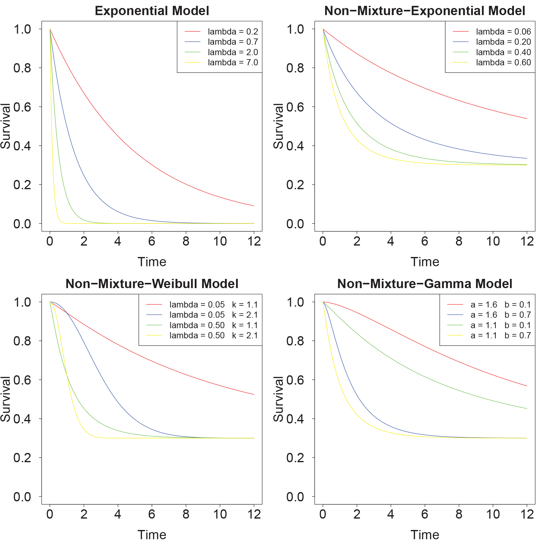
Examples of the four parametric survival models considered here. For the non-mixture models, we assumed a survival fraction of 0.3 throughout this figure.

3.1 Basic requirements

If Si0 are from the exponential class, one has to specify the rate parameters λi>0, i.e. Si0(t)=exp(−λit). The corresponding hazard functions hi for Si are then

(see Lemma 1 in Section B of the Appendix) which yields the hazard ratio

Thus time independence of the hazard ratio can only be achieved if

resulting in eq. (4). For clarification, this does not mean that we assume constant hazards (cf. eq. (5)) as it would be the case for the simple exponential model. Again, we consider the hypotheses

An estimator of the hazard ratio under λ1=λ2 can be defined by

(see Lemma 2 in Section B of the Appendix for more details).

3.2 Power estimate for the unconditional case

Similarly to eq. (1) in Section 2.2, one can start with

as the test statistic of interest, with Di=∑ji=1niΔi,ji and Oi′=∑ji=1ni1−exp−λiˆYi,ji. Here, Δi,ji for patient ji of group i indicates whether the patient is dead (Δi,ji=1) or censored (Δi,ji=0) whereas Yi,ji denotes the time of event or censoring. Using Theorem 3 in Section A of the Appendix, one can define the asymptotic power function via eq. (2) of Section 2.2. Here, the mean and variance under the null are given by μH0=0 and σH02=2n1−c11+log2c1−1 whereas under the alternative it holds that μH1(θ)=logθ and σH12(θ)=n1−c11+log2c1−1+n1−c1θ1+θlogc12−1.

3.3 Power estimate for the conditional case

Again, we consider the situation that data (D1,O1′,D2,O2′)=(d1,o1′,d2,o2′) is available from interim analysis. Let Di∗ denote the number of deaths and let O′i∗ be a function of the future observation time of group i counted from time of interim analysis until final analysis of the study in analogy to the definition of Oi′ at the beginning of Section 3.2. The conditional test statistic can be defined in analogy to eq. (6) in Section 3.2 by

With the help of Theorem 4 in Section A of the Appendix, the asymptotic conditional power function given (D1,O1′,D2,O2′)=(d1,o1′,d2,o2′), can be derived. Using eq. (3) of Section 2.3, corresponding means and variances under the null and the alternative are given by

3.4 Interpretation and comparison of unconditional power estimates

Here, we compare unconditional power estimates under the non-mixture exponential model with those of the simple exponential model. To illustrate the difference between the models, we choose α=5% and select three scenarios for (unconditional) power calculation. Sample size is kept fixed and was calculated to achieve a power of 80% for an initially chosen hazard ratio θ. The formula of Andersen [2] was used for this purpose. Power of the exponential and the non-exponential model were then calculated in dependence on modified hazard ratios. We considered the following scenarios:

Scenario 1: We fix the baseline survival rate c1=30% and choose an initial hazard ratio θ=0.872, resulting in a survival rate c2=35% for the experimental arm. According to Andersen, n=2481 patients are required for 80% power. Keeping the sample size constant and modifying the hazard ratio results in Figure 2 (left panel).

Scenario 2: We set the survival rate of the standard arm to c1=40% and choose an initial hazard ratio of θ=0.756, resulting in a survival rate of c2=50% for the experimental arm. Thus, simulations are performed for n=738 patients. The corresponding relation of hazard ratio and power is displayed in Figure 2 (mid panel).

Scenario 3: We assume a baseline survival rate c1=50% and set the initial hazard ratio to θ=0.621, resulting in a survival rate c2=65% for the experimental arm. Simulations are performed for n=337 patients. The resulting power plot is displayed in Figure 2 (right panel).

Assuming identical sample size and the same hazard ratio, power estimates under the non-mixture model are typically lower than those under the simple exponential model. Keeping the hazard ratio constant, the difference increases with baseline survival (cf. Figure 2). Survival rates can be chosen as one-, five-, or ten-year survival rates, for example, depending on the question of interest. These considerations also hold for the other non-mixture models considered here (non-mixture Weibull and non-mixture Gamma model, see below). In the situation of an interim analysis, available data might raise doubts regarding the survival model originally assumed. This might result in a revision of model parameters resulting in new power estimates. As expected, for both, exponential and non-mixture exponential models, power drops if the effect size is smaller than expected (see Figure 2).

Figure 2:

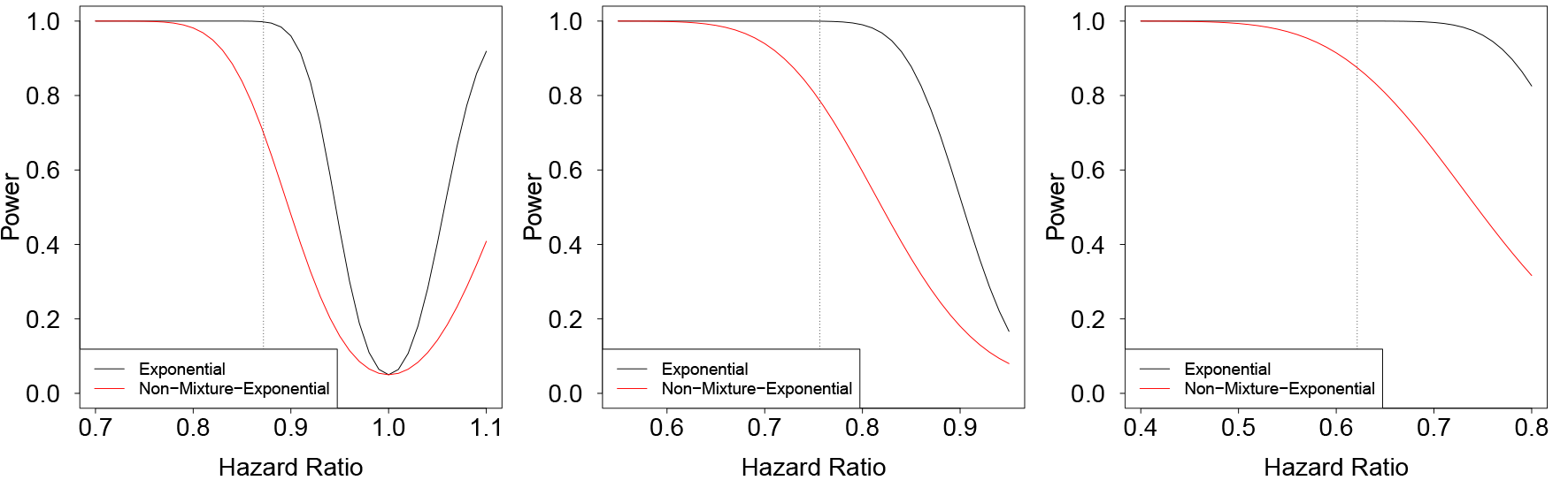
Power for the exponential (black) and the non-mixture exponential model (red) for three different scenarios. Left panel: c1=30%, n=2481. Mid panel: c1=40%, n=738. Right panel: c1=50%, n=337.

Conversely, our formulae can be used to re-calculate the sample sizes for the scenarios considered in Figure 2. Results are shown in Figure 3.

Figure 3:

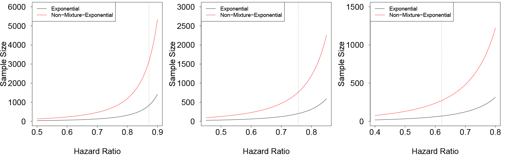
Sample size estimation of the scenarios considered in Figure 2. Sample size is calculated to achieve a power of 80%. Left panel: c1=30%. Mid panel: c1=40%. Right panel: c1=50%.

One can also interpret these results in terms of “information fraction”. Here, information fraction is defined as the ratio of the observed number of events at a given time point to the expected number of events at the end of the study. Then, the question is whether there are differences between the information fraction given a simple exponential model or given a non-mixture model. As mentioned above, event rates differ between both model types. The simple exponential model has a constant hazard whereas the hazard of the non-mixture model changes over time, being high at the early phase of the trial and decreasing to zero in the later phase of the trial. Thus, information fraction of an underlying non-mixture model will be higher at earlier time points and lower at later time points of a study compared to the information fraction under a simple exponential model at the same time points.

3.5 Empirical accuracy of the conditional power estimates

In this section, we illustrate accuracy of our conditional power formula for the non-mixture exponential model by performing a simulation study. The simulation study is implemented in the following way. First, we specify the parameters ci and λi of our non-mixture exponential model, and with it, the hazard ratio θ. Then, we simulate data for a fictive five-year clinical trial based on the above specified survival model under our proportional hazard assumption, i.e. λ1=λ2. Subject recruitment is distributed equally over study duration. We then simulate an interim analysis after 2.5 years by censoring events occurring after the time point of interim analysis. Interim data is used to calculate conditional power assuming a non-mixture exponential model. Further recruitment of subjects is considered within conditional power formula (equally until the end of study). For comparison, we apply the Wald test to the entire data set to decide whether the difference in survival at the end of the study is significant (value 1) or not (value 0). We repeat this simulation procedure 1,000 times and compare the average conditional power with the average of the Wald test decisions which can be interpreted as an empirical power. The following scenarios are considered:

Scenario 1: We choose a baseline survival rate c1=70% and a hazard ratio θ=0.626, resulting in a survival rate c2=80% for the experimental arm. The rate parameters are fixed at λ1=λ2=0.1. We perform simulations for n=500 patients. Conditional power by the non-mixture exponential model yields 32%, the percentage of significant Wald tests was the same (32%).

Scenario 2: We set the survival rate of the standard arm to c1=65% and choose a hazard ratio θ=0.377, resulting in a survival rate of c2=85% for the experimental arm. Finally, we choose λ1=λ2=0.2. Simulations are performed for n=250 patients. Conditional power based on the non-mixture exponential model is 67% while 70% of the Wald tests were significant.

Scenario 3: We assume a baseline survival rate c1=60% and a hazard ratio θ=0.318, resulting in a survival rate c2=85% for the experimental arm. The rate parameters are set to λ1=λ2=0.5. Simulations were performed for n=150 patients. Conditional power of the non-mixture exponential model yields 62% whereas 59% of the Wald tests are significant.

As one can see, conditional power estimates and Wald test results are in good agreement for the selected scenarios. To facilitate further simulations, we provide the corresponding R script as supplement material.

3.6 Alternative parametric assumptions for baseline hazard

The non-mixture exponential model might not be flexible enough to model the data adequately. Two possible alternatives are considered here: the non-mixture Weibull model and the non-mixture Gamma model. We introduce their notation now. The derivation of the (conditional) power functions is similar to that of the non-mixture exponential model. Results are presented in the Appendix.

4.1 The R package CP

We implemented the formulae derived in this paper in the framework of the R package CP which can be downloaded via CRAN. The function ConPwrExp contains the formulae for the exponential model without any cure fraction while the functions for the non-mixture models are ConPwrNonMixExp (exponential survival), ConPwrNonMixWei (Weibull-type survival) and ConPwrNonMixGamma (Gamma-type survival), respectively. A function for the comparison of these four models on the basis of Akaike’s information criterion (AIC) [6] is also included (CompSurvMod). Finally, conditional power according to Andersen (ConPwrExpAndersen) [2] can be calculated which is also based on an exponential model. Output comprises a summary of survival data of the interim analysis, AICs, parameter estimates, and estimates for the conditional power for the chosen model. Plots of the Kaplan-Meier curves and estimated parametric survival curves are provided. Further details and explanation of package parameters are presented in Table 1 and are available via the help pages of CP.

4.2 Clinical example

We applied our methods to an interim analysis of the highCHOEP trial of the German High-Grade Non-Hodgkin’s Lymphoma Study Group (DSHNHL) [7]. The question to be answered by this trial is whether there is a difference in survival between patients treated with either standard dosage chemotherapy (CHOEP) or dose-intensified chemotherapy (highCHOEP). Patients were between 18 and 60 years old and randomly received one of the above mentioned therapies as first-line treatment. At time of interim analysis, a total of 233 (CHOEP: 118, highCHOEP: 115) patients were analysed, revealing 69 (CHOEP: 33, highCHOEP: 36) death events and an aggregated observation time of 4306 (CHOEP: 2191, highCHOEP: 2115) months (see also Table 2).

The initial study was planned under an exponential survival model without cure fractions. A hazard ratio of 0.653 was assumed to be clinically relevant. We calculate conditional power for a total sample size of 389 patients assuming an accrual rate of 5.5 patients per month and group resulting in a final analysis after 14.2 months.

The function CompSurvMod of our R-package CP can now be used to calculate the conditional power for each of the models. Note that the hazard ratio translates into a ratio of log-cure fractions within our non-mixture models assuming proportional hazards. AIC can be used to decide which of the four models fits best. Lower AIC represents the better compromise between model complexity and fit. Calculated likelihoods, AICs, estimated parameters for survival functions and expected future observation times are shown in Table 3.

As one can see in Table 3, at time of interim analysis the estimated hazard ratios θˆ are close to 1.1 which is far away from the expected θ=0.653. With respect to the AIC, the non-mixture model with Weibull-type survival shows the best fit among the four models considered. Table 3 also shows, that compared to the exponential model, all three non-mixture models make a better compromise between data fitting and the number of additional parameters to be estimated. Moreover, the proportional hazard assumption for the non-mixture models, i.e. the equality of the rate, scale, and shape parameters of both groups is justified (Non-mixture-exponential: p = 0.9995, Non-mixture-Weibull: p = 0.3921, Non-mixture-Gamma: p = 0.1337, Likelihood ratio test). Figure 4 illustrates the Kaplan-Meier survival estimates of the interim data in comparison to the estimated parametric survival functions. Again, it can be recognised that the simple exponential model does not fit the data very well, in contrast to the non-mixture models. We present the conditional power curves in Figure 5, i.e. the dependence of power on the true effect size for the four models. The conditional power estimates for the planned effect (θ = 0.653) are: 39.2% for the exponential, 18.6% for the non-mixture exponential, 14.2% for the non-mixture Weibull, and 17.1% for the non-mixture Gamma model. Thus, a considerable difference in power estimates is obtained when switching to non-mixture models. The exponential model clearly over-estimates the conditional power due to over-estimation of the number of additional events. In contrast, differences in power estimates between the non-mixture models are relatively small. For interpreting these conditional power estimates it is necessary to provide further details regarding original study planning. The study was planned under the exponential model with 670 patients to achieve a power of 82%. Total sample size accounts for 10% of patients lost to follow-up or missing data. Due to an amendment prescribing additional treatment with the antibody Rituximab for every newly recruited patient, study analysis was performed for the 389 patients recruited thus far. Using the formula of Andersen, the reduced number of individuals results in a power of 59%. Performing the same calculations using the non-mixture exponential model results in a power of 95% for the 670 originally planned patients and 79% for the 389 available patients. Remembering our comparison of unconditional power estimates in Section 3.4, these results can be explained by two concurrent mechanisms: First, considering cure fractions results in fewer events and thus lower power in the longer perspective. However, events are generated more quickly under the non-mixture exponential model which could result in improved power at a shorter perspective. In other words, the survival curves assuming a simple exponential versus a non-mixture exponential model are typically intersecting if fitted to the same data (see also Figure 4). Thus, it is difficult to predict, which model results in the higher predicted power at a specified time point of final data analysis.

Figure 4:

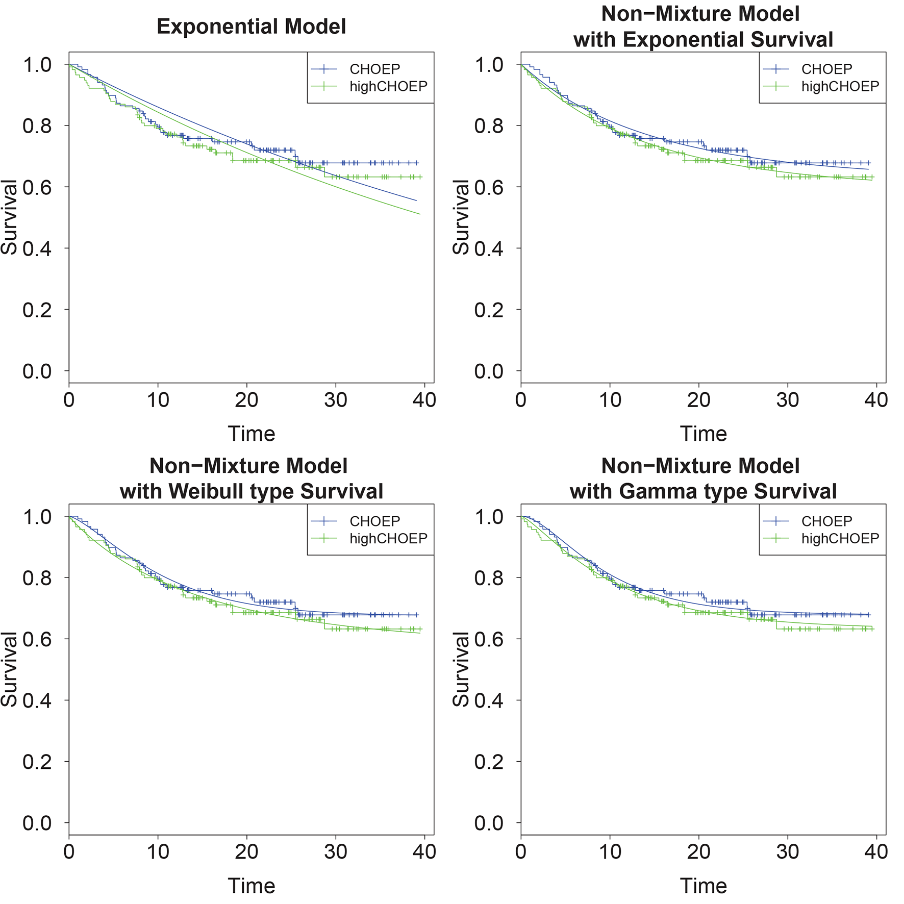
Comparison of parametric models and survival data: While the simple exponential model does not fit the data very well, the non-mixture models result in reasonable fits.

Figure 5:

Conditional power functions: We present conditional power estimates in dependence on the true effect size for each of the models.

5.1 Motivation of the work

Large clinical trials with survival endpoints are often time-consuming and costly. Therefore, interim analyses are common practice. If estimated effect size at time of interim analysis is far below the clinical expectation, conditional power might be a useful aid to evaluate futility of further recruitment which can result in premature termination of the trial. In case of a significant proportion of patients never experiencing an event, simple exponential survival models as proposed by Andersen [2] do not adequately describe the data. In the present paper, we derive conditional power formulae for three non-mixture models assuming cure fractions, namely those of exponential, Weibull, or Gamma type. We restricted our considerations to comparisons of two study arms and assume proportional hazards throughout the paper. Conditional power functions were implemented in an R package and are applied to a clinical data set.

5.2 Modelling Survival Data with Cure Fractions

There are three common types of modelling survival with cure fractions: The parametric, the semi-parametric, and the non-parametric approach, each of them having its own advantages and disadvantages [8]. Since the parametric approach offers a convenient way of testing proportional hazard assumptions and applying maximum likelihood methods for estimation purposes, this kind of modelling is chosen here. Asymptotic normality and unbiasedness of estimates in combination with the delta method allowed us to derive asymptotic distributions of the test statistic considered, which in our case, is the logarithm of the estimator of the hazard ratio.

Fitting piecewise exponential models could be an interesting alternative since it covers both cases, with and without cure fraction. It might also be appropriate for situations for which different event mechanisms could be expected, e.g. during and after an intense therapy. However, we believe that there are also disadvantages to this approach: First, the proportional hazard assumption is less obvious for this setting, especially if there are different event mechanisms to be considered. Without this assumption, the test statistic used in this paper is time dependent complicating all conditional power considerations. Second, the intervals of constant hazards need to be chosen and need to be identical for the treatment arms. This increases the number of free parameters to be determined or requires additional assumptions. Finally, conditional power relies on extrapolation of hazards. Considering a model of piece-wise constant hazards requires assumptions regarding the future of the piecewise behavior. Estimation of hazard ratios differ from exponential to non-mixture models. However, the relevant test statistic is the same. A problem could arise for non-mixture models if the regularity conditions required for asymptotic properties of maximum likelihood estimators are violated. This could occur due to the usage of quasi-probability density functions, i.e. survival functions bounded away from zero. Here, these regularity conditions are fulfilled (proof not shown).

Another approach of modelling survival is provided by the so-called mixture models. These models often give results very similar to those of the non-mixture models [9]. Further details can be found in Boag [10], Berkson and Gage [11], Sposto and Sather [12], and Sposto [13]. A completely different approach to estimating conditional power is via Bayesian methodology. This approach circumvents the issue of asymptotics, is often easier to calculate, and is directly interpretable. However, it faces the problem of specifying appropriate priors [14, 15].

5.3 Proportional Hazard Assumption

We assumed proportional hazards of the two study arms to be compared. In this sense, the non-mixture models as well as the exponential model are related to the Cox model with specified baseline hazard [16]; see Section 2.1 for the exponential model, eq. (5) for the non-mixture model with exponential survival, and Remark 3 for the non-mixture models with Weibull-type survival and Gamma-type survival. For all non-mixture models, proportional hazards imply that the hazard ratio equals the ratio of log-cure fractions. It allows applying the delta method to derive explicit formulae for conditional power. Without this assumption, the hazard ratio within the non-mixture models would be time dependent which causes problems when deriving the asymptotic distribution of the test statistic. Using likelihood methods, it is easy to evaluate appropriateness of the proportional hazard assumption. In our clinical example, this was the case for all assumed parametric families, cf. Section C.1 in the Appendix for the non-mixture exponential model. Due to the high flexibility of the parametric families considered, we believe that the proportional hazard assumption is appropriate for the majority of practical applications.

5.4 Practical Application

We applied our formulae to a data set of a clinical trial for which an interim analysis was performed. We observed considerable differences between power estimates based on a simple exponential model and our non-mixture models. The exponential model clearly did not fit the data well and resulted in an over-optimistic estimate of the conditional power. In contrast, differences between the non-mixture models were small. In general, non-mixture Weibull or non-mixture Gamma models offer a larger flexibility in modelling survival curves compared to the non-mixture exponential model. In practice, we expect larger differences between the exponential, the non-mixture exponential, and the non-mixture Weibull/Gamma models, while the difference between the non-mixture Weibull and the non-mixture Gamma model might be without practical relevance. We demonstrated that AIC can be used to decide which of the parametric models fits the data best. The analysis plan of clinical trials is usually prescribed in the study protocol. Therefore, we recommend the choice of an appropriate parametric model in the planning phase of a clinical trial. This could be identified e.g. on the basis of available historical data observed under the standard treatment. Here, AIC can be an aid for predetermination of a suitable survival model.

5.5 Aspects of Study Design

Our method allows to quantify the difference in power between the exponential and the non-mixture models. Furthermore, our formulae can be used to calculate sample sizes if the shape of the standard arm is known and a relevant hazard-ratio is specified. For conditional power analysis, we assumed that the time point of final analysis is fixed. However, event-driven designs are frequently used alternatives. These can be addressed with our formulae using the hazard functions estimated at the time point of interim analysis. The time point of final analysis is calculated on the basis of these hazards. Typically, this results in different time points for final analysis for different parametric models. E.g. for our example, final analysis was planned for 14.2 months after interim analysis. Alternatively, assuming an event-driven design, 108 events are required to achieve a power of 80%. Under the non-mixture exponential model, this is achieved at 15.2 months after interim analysis resulting in a conditional power of 19.4% (formerly 18.6%). For the exponential model, the time point of final analysis is 18.0 months after interim analysis resulting in a power of 57.0% (formerly 39.2%). Hence, differences in conditional power between models could even be larger for an event-driven design due to shifts in timing of the final analysis. However, this does not hold in general since the exponential model “generates” less events in the early phase but more events in the later phase compared to the non-mixture exponential model. We like to mention here that event-driven designs have the disadvantage that the required number of events might be unachievable if survival fractions or losses to follow-up are underestimated.

5.6 Non-inferiority Trials

The theory and methods proposed in this paper refer to superiority trials. Another important field of application might be non-inferiority trials. We plan to generalise our methods to this situation in the future. In contrast to superiority trials, a clinically relevant non-inferiority margin needs to be defined prior to sample size calculation. As a consequence, definition of test statistics, hypotheses, and derivations of conditional power formulae are more complex because of a composite null hypothesis. For this situation, the (conditional) power depends on both, the non-inferiority margin Δ and the hazard ratio θ.

5.7 Practical Interpretation of Conditional Power Estimates

When interpreting conditional power, one needs to keep in mind the following: Low conditional power indicates low chance to achieve a significant result at the end of the study. This suggests that termination of the study may be warranted. When the alternative is superior to the standard arm, this would result in high power. However, this does not necessarily imply that the trial should be continued. If the alternative is already significant at time of interim analysis (e.g. applying alpha spending), the trial must be terminated due to ethical reasons.

We like to remark that premature termination of clinical trials due to futility is a complex and serious issue. Conditional power is only one particular indicator which can be used. Confidence intervals of the observed effect sizes – here, the observed hazard ratio – is another measure to decide whether the originally postulated hazard ratio is realistic or if the trial should be stopped for futility. Defining strict boundaries for study termination is difficult for both methods as it depends on time and frequency of interim analyses. Moreover, there are several non-statistical aspects which have to be considered: Premature termination of the study can be decided for the above mentioned ethical reasons or if other treatments become standard. Practical reasons could be an over-estimated recruitment rate or an under-estimated loss to follow-up. Economic aspects could also be relevant, e.g. expensive experimental treatments showing low benefit could more likely be discarded. Stopping for futility is often a mixture of statistical methods and other aspects. In particular, for our clinical example, the major reason for stopping the trial was not the reduced conditional power at interim analysis but the fact that treating patients without the novel drug Rituximab was considered ethically not acceptable. However, we believe that in general conditional power is a useful method to support decision-making in clinical trials.

References

1. Lambert PC. Modeling of the cure fraction in survival studies. Stata J. 2007;7:351–375.10.1177/1536867X0700700304Search in Google Scholar
2. Andersen PK. Conditional power calculations as an aid in the decision whether to continue a clinical trial. Control Clin Trials. 1987;8:67–74.10.1016/0197-2456(87)90027-4Search in Google Scholar
3. Martinez EZ, Achcar JA, Jácome AA, Santos JS. Mixture and non-mixture cure fraction models based on the generalized modified Weibull distribution with an application to gastric cancer data. Compute Methods Programs Biomed. 2013;112:343–355.10.1016/j.cmpb.2013.07.021Search in Google Scholar
4. Tsodikov AD, Ibrahim JG, Yakovlev AY. Estimating cure rates from survival data: an alternative to two-component mixture models. J Am Stat Assoc. 2003;98:1063–1078.10.1198/01622145030000001007Search in Google Scholar
5. Tsodikov A, Loeffler M, Yakovlev A. A cure model with time-changing risk factor: an application to the analysis of secondary Leukaemia. Stat Med. 1998;17:27–40.10.1002/(SICI)1097-0258(19980115)17:1<27::AID-SIM720>3.0.CO;2-QSearch in Google Scholar
6. Akaike H. A new look at the statistical model identification. IEEE Trans Automatic Control. 1974;19:716–723.10.1007/978-1-4612-1694-0_16Search in Google Scholar
7. Pfreundschuh M, Zwick C, Zeynalova S, Duehrsen U, Pflueger KH, Vrieling T,et al. Dose-escalated CHOEP for the treatment of young patients with aggressive non-Hodgkin’s lymphoma: II. Results of the randomized high-CHOEP trial of the German High-Grade Non-Hodgkin’s Lymphoma Study Group (DSHNHL). Ann Oncol. 2007;19:545–552.10.1093/annonc/mdm514Search in Google Scholar
8. Altman DG, Bland JM. Parametric v non-parametric methods for data analysis. BMJ. 2009;338:a3167.10.1136/bmj.a3167Search in Google Scholar
9. Achcar JA, Coelho-Barros EA, Mazucheli J. Cure fraction models using mixture and non-mixture models. Tatra Mountains Math Publications. 2012;51:1–9.10.2478/v10127-012-0001-4Search in Google Scholar
10. Boag JW. Maximum likelihood estimates of the proportion of patients cured by cancer therapy. J R Stat Soc Ser B Method. 1949;11:15–53.10.1111/j.2517-6161.1949.tb00020.xSearch in Google Scholar
11. Berkson J, Gage RP. Survival curve for cancer patients following treatment. J Am Stat Assoc. 1952;47:501–515.10.1080/01621459.1952.10501187Search in Google Scholar
12. Sposto R, Sather HN. Determining the duration of comparative clinical trials while allowing for cure. J Chronic Dis. 1985;38:683–690.10.1016/0021-9681(85)90022-0Search in Google Scholar
13. Sposto R. Cure model analysis in cancer: an application to data from the children’s cancer group. Stat Med. 2002;21:293–312.10.1002/sim.987Search in Google Scholar PubMed
14. Ibrahim JG, Chen MH, Sinha D. Bayesian semiparametric models for survival data with a cure fraction. Biometrics. 2001;57:383–388.10.1111/j.0006-341X.2001.00383.xSearch in Google Scholar
15. Yin G, Ibrahim JG. A general class of bayesian survival models with zero and nonzero cure fractions. Biometrics. 2005;61:403–412.10.1111/j.1541-0420.2005.00329.xSearch in Google Scholar PubMed
16. Cox DR. Regression models and life-tables. J R Stat Soc Ser B Methodol. 1972;34:187–220.10.1007/978-1-4612-4380-9_37Search in Google Scholar
17. Greene WH. Econometric analysis. Upper Saddle River:Prentice Hall, 2003.Search in Google Scholar
18. Serfling RJ. Approximation theorems of mathematical statistics. New York:John Wiley & Sons, 1980.10.1002/9780470316481Search in Google Scholar
19. Klein JP, Moeschberger ML. Survival analysis. Techniques for censored and truncated data. New York: Springer Science+Business Media, 2005.Search in Google Scholar
Supplemental Material
The online version of this article (DOI:ijb-2015-0073) offers supplementary material, available to authorized users.
© 2017 Walter de Gruyter GmbH, Berlin/Boston
Articles in the same Issue
- Commentary
- Big Data, Small Sample
- Research Articles
- Parameter Estimation of a Two-Colored Urn Model Class
- Combinatorial Mixtures of Multiparameter Distributions: An Application to Bivariate Data