Influence Re-weighted G-Estimation
-
Benjamin Rich
 and
David A. Stephens
and
David A. Stephens

Abstract
Individualized medicine is an area that is growing, both in clinical and statistical settings, where in the latter, personalized treatment strategies are often referred to as dynamic treatment regimens. Estimation of the optimal dynamic treatment regime has focused primarily on semi-parametric approaches, some of which are said to be doubly robust in that they give rise to consistent estimators provided at least one of two models is correctly specified. In particular, the locally efficient doubly robust g-estimation is robust to misspecification of the treatment-free outcome model so long as the propensity model is specified correctly, at the cost of an increase in variability. In this paper, we propose data-adaptive weighting schemes that serve to decrease the impact of influential points and thus stabilize the estimator. In doing so, we provide a doubly robust g-estimator that is also robust in the sense of Hampel (15).
1 Introduction
The “personalization” of medicine is an area that is receiving ever-growing attention from medical practitioners, statisticians, and computer scientists, to name but some of the interested parties. The U.S. Food and Drug Administration refers to this personalization as “tailoring medical treatment to […] a patient’s genetic, anatomical, and physiological characteristics”, approaches which are “allowing patients to be treated and monitored more precisely and effectively and in ways that better meet their individual needs” [1]. Within the statistics literature, there have been a great variety of methods proposed for estimating optimal personalized treatment strategies, also known as dynamic treatment regimens (DTRs), from regression-based approaches (Schulte et al. [2] provide an excellent review) to classification-based algorithms (e.g. Zhang et al. [3], Zhao [4]). Although there have been some fully parametric approaches considered [5, 6], the majority of estimation approaches have been semi-parametric (e.g. Murphy [7], Orellana et al. [8], Robins [9], van der Laan and Petersen [10], Zhang et al. [11]).
Semi-parametric methods frequently give rise to estimators that are locally efficient, meaning that the estimator’s asymptotic variance achieves the semi-parametric efficiency bound if the true data generating distributing happens to belong to a certain class, yet remain consistent and asymptotically normal (CAN) under broader conditions. This is true, in particular, for any estimator that bears the designation “doubly robust” [12]. In causal inference, doubly robust estimators typically involve the specification of two nuisance models, one modelling the treatment assignment mechanism in terms of confounders (e.g. a propensity score [13]), the other modelling the outcome in terms of confounders and risk factors. The common approach is to specify parametric working models for these nuisance models, though non-parametric alternatives (e.g. trees) could equally be viable. The estimator achieves semi-parametric efficiency if all parametric components, including both nuisance models, are specified correctly.
Depending on the context, one or the other nuisance model may be easier to specify correctly. Randomized trials are one setting where the treatment assignment mechanism is known, for instance. In a pharmacoepidemiological context, it may be possible to construct a realistic propensity score model through consultation with clinicians who understand the factors that are considered in making treatment decisions. The effect of the treatment on a clinical outcome may be more difficult to model as it involves complex biological systems, interactions with genes and environment, etc.; it is plausible that partial model misspecification occurs quite commonly in practice. Since standard estimators are not efficient under partial misspecification, it is natural to look for ways to improve on them. In particular, it would be useful to find a means of making the doubly-robust estimators more stable – further “robustifying” such estimators to influential observations.
In this work, we undertake a data-adaptive approach to increasing the stability of the doubly-robust g-estimators of optimal dynamic treatment regimen structural nested mean models (SNMMs) [9]. In the next section, we review g-estimators of DTRs and present results which will be used to develop our proposed approach, in which the g-estimation equation at each interval is modified to incorporate a weight determined by a prediction of the influence of the individual at that interval.
2 Background
2.1 G-estimation of SNMMs for DTRs
A dynamic treatment regimen is a sequence of functions
Two key features of the blip function are (1) the blip function evaluated at
where
where
We shall now consider a partially misspecified setting, namely we shall suppose that while the treatment or propensity model
2.2 Weighting in estimating equations: some general results
Suppose that we have observed i.i.d. data
Standard M-estimator theory Tsiatis [16] tells us that we can construct an (unweighted) estimator of
and asymptotic variance given by
Now, let
First, we observe that the usual Taylor expansion gives
where
Where Z has the standard normal distribution.
If
We now give a sufficient condition for the consistency of
If the conditional expectation
Proof. If the weights are not data-dependent, then by iterated expectation:
so the usual M-estimator theory also applies to
3 Weighting within the g-estimation framework
For each interval
for
The inner expectation can be shown to zero under the assumptions of consistency and sequential randomization and a correctly specified propensity model.
3.1 Influence-based weighting schemes
Under correct specification of the treatment-free outcome model, Robins [9] gives an expression for a weight function for g-estimation that is optimal in an efficiency sense (under some further assumptions). The weight is proportional to the inverse of the conditional variance
We propose a different approach to constructing weights which seeks to stabilize the standard estimator in a manner which does not depend on correct model specification and can improve its performance as measured by mean squared error in certain cases (as we will see in a simulation study of Section 4).
Data points that are candidates to receive reduced weights in the estimating equation are points with high sample influence. Hinkley [19] and Krasker and Welsch [20] discuss the use of weights constructed as functions of the sample influence in the context of robust regression estimators. Here, the proposal is to identify data points that are highly influential in the estimation of the parameter of interest, and reducing the influence of those individuals through subsequent re-weighting, will stabilize the estimation and make it more robust to misspecification of the nuisance treatment-free outcome model. The sample influence of a data point is, however, constructed from all the available data. Thus, while it is straightforward to describe an algorithm in which weights are constructed such that the weight for individual I is inversely proportional to the sample influence of individual i on the estimate of
3.2 Influence measures in g-estimation
Influence refers to the stability of statistics (e.g. estimators) to perturbations of the data. The mathematical object used to describe the asymptotic stability of an estimator is the influence function (IF) (Hampel et al. [15], Tsiatis [16], Cook and Weisberg [21]). The idea is to consider the distribution function F from which the observed data
where
The IF is a useful theoretical tool, but its use in practice for model diagnostics is limited since it depends on the true data generating distribution, which is only available under correct model misspecification and infinite samples. More useful for diagnostics is the finite sample analogue of the IF, obtained through the jackknife (leave-one-out) approach. Consider
Then, the sample influence (SI) of observation i is obtained from (2) by setting
In standard outcome regression such as
DFBETA
DFFIT
Cook’s distance
for a symmetric and positive definite matrix
Consider now the g-estimator
and
3.3 Influence re-weighted g-estimation
The procedure begins with an initial solution to the weighted g-estimating equations, using some initial set of weights that we denote
where
where
In the proposed family
3.4 Re-weighting “inside-the-loop” and “outside-the-loop”
When g-estimation is applied recursively, there are two different variants of the algorithm for computing a re-weighted estimator depending on the ordering of the calculations. We have called them “inside-the-loop” and “outside-the-loop”, making reference to a programming loop with a loop index j that goes down from K to 1. The two variants are sketched in pseudo-code in Figure 1. Essentially, the distinction is whether the initial estimate of

Algorithms for re-weighting “inside-the-loop” (a) and “outside-the-loop” (b).
3.5 Consistent re-weighting
As stated previously, the estimation procedure described above may have undesirable properties. In particular, because the terms of the estimating equations are not i.i.d. and the conditions of Lemma 1 do not necessarily hold, consistency of the estimator is not assured. We now propose a simple way to adapt the procedure and obtain a different estimator, similarly motivated, that is not subject to these difficulties.
The idea is to construct a set of weights such that the weight for individual i at interval j is a function of the history
The challenge with this approach is in constructing predictive models for the sample influence at each interval. We approached this in two different ways: direct prediction of the compound influence
Unlike the compound influence
Yet a third approach that we considered was to orthogonalize the individual components before prediction. This allows for better prediction in the case where the individual components of
Once the prediction
4 Simulations
Simulations were performed using the basic approach described in Moodie, Richardson, and Stephens [26] but with different parameter settings. The basic setup for the simulation is presented in Figure 2. Note that in this data generating model, the outcome Y can depend on treatments

The basic setup used for simulating data from an SNMM with two treatment intervals.
Simulation scenarios.
| Scenario | Parameter settings |
| 1a | |
| 1b | Like scenario 1a but with |
| 1c | Like scenario 1a but with |
| 1d | Like scenario 1a but with |
| 1e | Like scenario 1a but with |
| and | |
| 1f | Like scenario 1e but with |
Sample sizes
First, simple linear models are considered for the specification of the nuisance treatment-free outcome models, specifically:
Because
For PIBW estimators, influence was predicted using flexible spline models. Specifically, we regressed
The knots for the B-splines were chosen automatically by the bs( ) function in R (an internal knot at the median, and boundary knots at the minimum and maximum by default).
We studied the effect of the tuning parameter
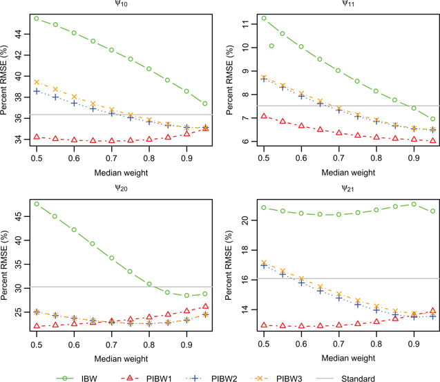
Percent RMSE (based on 100 replications) vs. median weight for scenario 1f with sample size
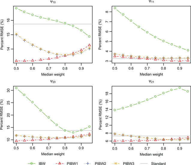
Percent RMSE (based on 100 replications) vs. median weight for scenario 1f with sample size
Based on these findings, the tuning parameter was set to achieve a median weight of 0.7 and 0.9 at intervals 2 and 1 respectively for PIBW1, 0.9 and 0.95 at intervals 2 and 1 respectively for PIBW2 and PIBW3, and 0.97 and 0.99 at intervals 2 and 1 respectively for IBW. Then for each scenario 1,000 new simulation repetitions were performed (using a different seed for the random number generator). The simulation results for scenarios 1a–1f are summarized in Tables 2 and 3 for the two sample sizes
Performance of weighted estimators compared to standard and efficient estimators for scenarios 1a–1f measured by percent RMSE and RMSE relative to the standard estimator (in parentheses) based on 1,000 data sets of size
| Parameter (truth) | Estimator | Scenario | |||||||||||
| 1a | 1b | 1c | 1d | 1e | 1f | ||||||||
| Standard | 28.43 | (1.00) | 12.52 | (1.00) | 29.66 | (1.00) | 35.93 | (1.00) | 28.50 | (1.00) | 37.44 | (1.00) | |
| Efficient | 26.55 | (0.93) | 0.87 | (0.07) | 26.65 | (0.90) | 27.00 | (0.75) | 25.49 | (0.89) | 25.94 | (0.69) | |
| IBW | 28.96 | (1.02) | 13.11 | (1.05) | 30.48 | (1.03) | 37.04 | (1.03) | 28.71 | (1.01) | 36.18 | (0.97) | |
| PIBW1 | 28.52 | (1.00) | 10.95 | (0.87) | 29.28 | (0.99) | 35.32 | (0.98) | 27.81 | (0.98) | 34.87 | (0.93) | |
| PIBW2 | 29.22 | (1.03) | 10.34 | (0.83) | 29.67 | (1.00) | 34.91 | (0.97) | 28.69 | (1.01) | 35.15 | (0.94) | |
| PIBW3 | 29.22 | (1.03) | 10.42 | (0.83) | 29.67 | (1.00) | 34.95 | (0.97) | 28.72 | (1.01) | 35.20 | (0.94) | |
| Standard | 10.55 | (1.00) | 6.07 | (1.00) | 11.52 | (1.00) | 8.05 | (1.00) | 10.96 | (1.00) | 7.75 | (1.00) | |
| Efficient | 9.46 | (0.90) | 0.32 | (0.05) | 10.12 | (0.88) | 5.67 | (0.70) | 9.34 | (0.85) | 4.88 | (0.63) | |
| IBW | 11.19 | (1.06) | 6.38 | (1.05) | 12.07 | (1.05) | 9.72 | (1.21) | 10.79 | (0.98) | 7.28 | (0.94) | |
| PIBW1 | 10.61 | (1.01) | 4.89 | (0.81) | 11.59 | (1.01) | 7.92 | (0.98) | 10.34 | (0.94) | 6.78 | (0.88) | |
| PIBW2 | 11.24 | (1.07) | 4.35 | (0.72) | 12.09 | (1.05) | 7.57 | (0.94) | 11.25 | (1.03) | 6.98 | (0.90) | |
| PIBW3 | 11.22 | (1.06) | 4.36 | (0.72) | 12.12 | (1.05) | 7.59 | (0.94) | 11.28 | (1.03) | 6.99 | (0.90) | |
| Standard | 16.54 | (1.00) | 12.13 | (1.00) | 14.52 | (1.00) | 21.87 | (1.00) | 18.10 | (1.00) | 30.95 | (1.00) | |
| Efficient | 11.50 | (0.70) | 0.39 | (0.03) | 11.16 | (0.77) | 12.69 | (0.58) | 10.42 | (0.58) | 10.95 | (0.35) | |
| IBW | 16.74 | (1.01) | 11.42 | (0.94) | 14.68 | (1.01) | 21.48 | (0.98) | 18.32 | (1.01) | 31.25 | (1.01) | |
| PIBW1 | 16.04 | (0.97) | 11.00 | (0.91) | 13.91 | (0.96) | 23.43 | (1.07) | 15.91 | (0.88) | 25.01 | (0.81) | |
| PIBW2 | 16.33 | (0.99) | 11.46 | (0.95) | 14.21 | (0.98) | 21.42 | (0.98) | 16.87 | (0.93) | 25.70 | (0.83) | |
| PIBW3 | 16.37 | (0.99) | 11.47 | (0.95) | 14.24 | (0.98) | 21.45 | (0.98) | 16.91 | (0.93) | 25.80 | (0.83) | |
| Standard | 15.68 | (1.00) | 13.41 | (1.00) | 17.34 | (1.00) | 14.16 | (1.00) | 15.36 | (1.00) | 15.63 | (1.00) | |
| Efficient | 9.95 | (0.63) | 0.32 | (0.02) | 11.11 | (0.64) | 7.07 | (0.50) | 7.92 | (0.52) | 4.74 | (0.30) | |
| IBW | 20.32 | (1.30) | 17.86 | (1.33) | 22.47 | (1.30) | 22.51 | (1.59) | 16.00 | (1.04) | 19.62 | (1.26) | |
| PIBW1 | 15.43 | (0.98) | 12.22 | (0.91) | 16.11 | (0.93) | 14.88 | (1.05) | 13.46 | (0.88) | 13.06 | (0.84) | |
| PIBW2 | 14.88 | (0.95) | 10.46 | (0.78) | 15.58 | (0.90) | 12.86 | (0.91) | 13.69 | (0.89) | 12.88 | (0.82) | |
| PIBW3 | 14.89 | (0.95) | 10.48 | (0.78) | 15.68 | (0.90) | 12.92 | (0.91) | 13.69 | (0.89) | 12.94 | (0.83) | |
Performance of weighted estimators compared to standard and efficient estimators for scenarios 1a–1f measured by percent RMSE and RMSE relative to the standard estimator (in parentheses) based on 1,000 data sets of size
| Parameter (truth) | Estimator | Scenario | |||||||||||
| 1a | 1b | 1c | 1d | 1e | 1f | ||||||||
| Standard | 12.34 | (1.00) | 5.19 | (1.00) | 12.50 | (1.00) | 16.06 | (1.00) | 12.68 | (1.00) | 15.78 | (1.00) | |
| Efficient | 11.31 | (0.92) | 0.39 | (0.08) | 11.37 | (0.91) | 12.16 | (0.76) | 11.62 | (0.92) | 11.24 | (0.71) | |
| IBW | 12.73 | (1.03) | 5.71 | (1.10) | 12.87 | (1.03) | 16.58 | (1.03) | 12.81 | (1.01) | 15.26 | (0.97) | |
| PIBW1 | 12.24 | (0.99) | 4.51 | (0.87) | 12.35 | (0.99) | 15.91 | (0.99) | 12.55 | (0.99) | 14.90 | (0.94) | |
| PIBW2 | 12.42 | (1.01) | 4.26 | (0.82) | 12.53 | (1.00) | 15.63 | (0.97) | 12.77 | (1.01) | 14.97 | (0.95) | |
| PIBW3 | 12.43 | (1.01) | 4.30 | (0.83) | 12.53 | (1.00) | 15.64 | (0.97) | 12.78 | (1.01) | 14.98 | (0.95) | |
| Standard | 4.81 | (1.00) | 2.60 | (1.00) | 4.86 | (1.00) | 3.45 | (1.00) | 4.80 | (1.00) | 3.08 | (1.00) | |
| Efficient | 4.32 | (0.90) | 0.14 | (0.06) | 4.32 | (0.89) | 2.50 | (0.73) | 4.15 | (0.87) | 2.08 | (0.68) | |
| IBW | 5.72 | (1.19) | 3.59 | (1.38) | 5.59 | (1.15) | 6.59 | (1.91) | 4.79 | (1.00) | 2.92 | (0.95) | |
| PIBW1 | 4.70 | (0.98) | 1.76 | (0.67) | 4.72 | (0.97) | 3.39 | (0.98) | 4.56 | (0.95) | 2.68 | (0.87) | |
| PIBW2 | 4.95 | (1.03) | 1.74 | (0.67) | 5.12 | (1.05) | 3.23 | (0.94) | 4.88 | (1.02) | 2.85 | (0.93) | |
| PIBW3 | 4.95 | (1.03) | 1.75 | (0.67) | 5.12 | (1.05) | 3.24 | (0.94) | 4.88 | (1.02) | 2.85 | (0.93) | |
| Standard | 6.86 | (1.00) | 5.03 | (1.00) | 6.99 | (1.00) | 9.72 | (1.00) | 8.33 | (1.00) | 13.62 | (1.00) | |
| Efficient | 4.98 | (0.73) | 0.18 | (0.04) | 5.08 | (0.73) | 5.51 | (0.57) | 4.88 | (0.59) | 4.96 | (0.36) | |
| IBW | 6.84 | (1.00) | 5.24 | (1.04) | 6.84 | (0.98) | 10.15 | (1.04) | 8.67 | (1.04) | 15.42 | (1.13) | |
| PIBW1 | 6.64 | (0.97) | 4.58 | (0.91) | 6.51 | (0.93) | 10.24 | (1.05) | 7.17 | (0.86) | 10.88 | (0.80) | |
| PIBW2 | 6.79 | (0.99) | 4.72 | (0.94) | 6.59 | (0.94) | 9.63 | (0.99) | 7.63 | (0.92) | 11.53 | (0.85) | |
| PIBW3 | 6.79 | (0.99) | 4.72 | (0.94) | 6.59 | (0.94) | 9.65 | (0.99) | 7.64 | (0.92) | 11.57 | (0.85) | |
| Standard | 7.44 | (1.00) | 5.60 | (1.00) | 7.61 | (1.00) | 6.60 | (1.00) | 6.52 | (1.00) | 6.87 | (1.00) | |
| Efficient | 4.10 | (0.55) | 0.13 | (0.02) | 4.72 | (0.62) | 2.91 | (0.44) | 3.28 | (0.50) | 1.94 | (0.28) | |
| IBW | 15.99 | (2.15) | 15.84 | (2.83) | 16.34 | (2.15) | 19.87 | (3.01) | 8.98 | (1.38) | 15.42 | (2.24) | |
| PIBW1 | 6.98 | (0.94) | 5.11 | (0.91) | 6.80 | (0.89) | 7.09 | (1.07) | 5.76 | (0.88) | 5.27 | (0.77) | |
| PIBW2 | 6.68 | (0.90) | 4.51 | (0.81) | 6.60 | (0.87) | 5.62 | (0.85) | 6.16 | (0.94) | 5.68 | (0.83) | |
| PIBW3 | 6.68 | (0.90) | 4.52 | (0.81) | 6.60 | (0.87) | 5.63 | (0.85) | 6.16 | (0.94) | 5.67 | (0.82) | |
We observe that across these simulation scenarios, there was either no real benefit or a modest reduction in variability from using the PIBW estimators versus the standard unweighted estimator. When the PIBW weighting procedure did appear to be beneficial, most of the benefit was observed at the second interval (scenario 1b is an exception), and in the estimation of
We can gain some insight into why the PIBW estimators performed better than the standard estimator in some scenarios and not in others by looking at the residual plots obtained from fitting the standard estimator. Figure 5 shows plots of residuals at intervals 1 and 2 versus
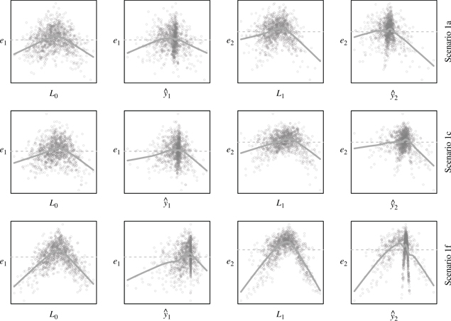
Residual plots for simulation scenarios 1a, 1c and 1f for the standard (unweighted) g-estimator fit using a misspecified linear treatment-free outcome model. A typical data set of size
So far, simple linear models were considered for the specification of the nuisance treatment-free outcome models. Because the true treatment-free outcome model in this simulation setup is piecewise linear (except in the null scenario 2, where it is linear), the linear treatment-free outcome models may fit quite poorly. In fact, for scenario 1f where the proposed estimators performed best, simple residual plots as described by Rich et al. [14] would have revealed the poor fit (Figure 5). Thus, we repeated the previous simulations using a more flexible treatment-free outcome model, specifically:
where
5 Discussion
Locally efficient doubly robust g-estimation is robust to misspecification of the treatment-free outcome model so long as the propensity model is specified correctly, but a price for misspecification is paid in efficiency. The weighting schemes proposed in this manuscript are an attempt to counteract this efficiency loss using weights that are adaptively derived to decrease the impact of influential points and thus stabilize the estimator.
The applicability of this methodology depends on how well or how poorly the misspecified treatment-free outcome model approximates the true model, and correspondingly how close the standard estimator is to the efficient estimator. The residual diagnostics given by Rich et al. [14] are a means of assessing the goodness of fit and in some cases may suggest ways of improving the estimator through alternative specifications of the treatment-free outcome model. In some cases, this may obviate the need for the re-weighting approach, but in more complex, high-dimensional settings, the diagnostic techniques may be insufficient to fully address treatment-free outcome model misspecification so the re-weighting approach may prove to be useful. The simulation results presented in this manuscript suggest that in some settings the use of PIBW estimators can result in important decreases in the variability of the estimator (a 15–20% reduction in RMSE or more was observed in some scenarios).
The re-weighting procedure described involves solving the g-estimating equation at interval j, determining the influence of each individual
The choice of the tuning parameter
Acknowledgements
This work was carried out when the first author was studying in the Department of Epidemiology, Biostatistics, and Occupational Health of McGill University, and receiving support from the Natural Sciences and Engineering Research Council (NSERC) of Canada. Drs. Moodie and Stephens acknowledge support of NSERC of Canada. Dr. Moodie is supported by a Chercheur-Boursier junior 2 career award from the Fonds de recherche du Quebec-Sante (FRQ-S).
References
1. and Drug Administration, U. S. F. Paving the way for personalized medicine FDA’s role in a new era of medical product development, 2013. Available at: http://www.fda.gov/downloads/scienceresearch/specialtopics/personalizedmedicine/ucm372421.pdf.Search in Google Scholar
2. Schulte PJ, Tsiatis AA, Laber EB, Davidian M. Q- and A-learning methods for estimating optimal dynamic treatment regimes. Stat Sci 2014;29:640–661.10.1214/13-STS450Search in Google Scholar PubMed PubMed Central
3. Zhang B, Tsiatis A, Davidian M, Zhang M, Laber E. Estimating optimal treatment regimes from a classification perspective. Stat 2012a;1:103–14.10.1002/sta.411Search in Google Scholar PubMed PubMed Central
4. Zhao Y, Zeng D, Rush A, Kosorok M. Estimating individual treatment rules using outcome weighted learning. J Am Stat Assoc 2012;107:1106–18.10.1080/01621459.2012.695674Search in Google Scholar PubMed PubMed Central
5. Arjas E, Saarela O. Optimal dynamic regimes presenting a case for predictive inference. Int J Biostat 2010;6: Article 10.10.2202/1557-4679.1204Search in Google Scholar PubMed PubMed Central
6. Zajonc T. Bayesian inference for dynamic treatment regimes mobility, equity, and efficiency in student tracking. J Am Stat Assoc 2012;107:80–92.10.1080/01621459.2011.643747Search in Google Scholar
7. Murphy SA. Optimal dynamic treatment regimes. J R Stat Soc Ser B (Stat Methodol) 2003;65:331–55. Available at: http://doi.wiley.com/10.1111/1467-9868.00389.10.1111/1467-9868.00389Search in Google Scholar
8. Orellana L, Rotnitzky A, Robins JM. Dynamic regime marginal structural mean models for estimation of optimal dynamic treatment regimes, part I main content. Int J Biostat 2010;6. Available at: http://www.bepress.com/ijb/vol6/iss2/8/.10.2202/1557-4679.1200Search in Google Scholar
9. Robins JM. Optimal structural nested models for optimal sequential decisions. In: DY Lin, PJ Heagerty, editors. Proceedings of the second Seattle symposium in biostatistics analysis of correlated data. Springer, 2004:189–326. Available at: http://www.biostat.harvard.edu/robins/publications/seattlemay04final.pdf.10.1007/978-1-4419-9076-1_11Search in Google Scholar
10. van der Laan MJ, Petersen ML. Causal effect models for realistic individualized treatment and intention to treat rules. Int J Biostat 2007;3. Available at: http://www.pubmedcentral.nih.gov/articlerender.fcgi?artid=2613338%26tool=pmcentrez%26rendertype=abstract.10.2202/1557-4679.1022Search in Google Scholar PubMed PubMed Central
11. Zhang B, Tsiatis A, Laber E, Davidian M. A robust method for estimating optimal treatment regimes. Biometrics 2012b;68:1010–18.10.1111/j.1541-0420.2012.01763.xSearch in Google Scholar PubMed PubMed Central
12. Tan Z. Bounded, efficient and doubly robust estimation with inverse weighting. Biometrika 2010;97:661–82. Available at: http://biomet.oxfordjournals.org/cgi/doi/10.1093/biomet/asq035.10.1093/biomet/asq035Search in Google Scholar
13. Rosenbaum PR, Rubin DB. The central role of the propensity score in observational studies for causal effects. Biometrika 1983;70:41–55. Available at: http://biomet.oxfordjournals.org/content/70/1/41.short.10.21236/ADA114514Search in Google Scholar
14. Rich B, Moodie EEM, Stephens DA, Platt RW. Model checking with residuals for g-estimation of optimal dynamic treatment regimes. Int J Biostat 2010;6. Available at: http://www.bepress.com/ijb/vol6/iss2/12/.10.2202/1557-4679.1210Search in Google Scholar PubMed
15. Hampel FR, Ronchetti EM, Rousseeuw PJ, Stahel WA. Robust statistics the approach based on influence functions. New York: Wiley, 1986. Available at: http://www.lavoisier.fr/notice/frIWOR363ASRWLKO.html.Search in Google Scholar
16. Tsiatis AA. Semiparametric theory and missing data. New York: Springer, 2006. Available at: http://books.google.ca/books?hl=en26lr=%26id=xqZFi2EMB40C26oi=fnd26pg=PR726dq=tsiatis+semiparametric+missing%26ots=NCe_abJdMv26sig=Bj8z0t1ke6U11qhdIWM5N6OEMRs.Search in Google Scholar
17. Newey WK. Semiparametric efficiency bounds. J Appl Econ 1990. Available at: http://www3.interscience.wiley.com/journal/112749856/abstract.10.1002/jae.3950050202Search in Google Scholar
18. Joffe MM, Brensinger C. Weighting in instrumental variables and G-estimation. Stat Med 2003;22:1285–303. Available at: http://www.ncbi.nlm.nih.gov/pubmed/12687655.10.1002/sim.1380Search in Google Scholar PubMed
19. Hinkley DV. Jackknifing in unbalanced situations. Technometrics 1977;19:285–92. Available at: http://www.jstor.org/stable/1267698.10.1080/00401706.1977.10489550Search in Google Scholar
20. Krasker WS, Welsch RE. Efficient bounded-influence regression estimation. J Am Stat Assoc 1982;77:595–604. Available at: http://www.jstor.org/stable/2287719.10.1080/01621459.1982.10477855Search in Google Scholar
21. Cook RD, Weisberg S. Residuals and influence in regression, New York Chapman and Hall, 1982. Available at: http://purl.umn.edu/37076.Search in Google Scholar
22. Seber GAF, Lee AJ. Linear regression analysis, 2nd ed. Hoboken, NJ: Wiley, 2003.10.1002/9780471722199Search in Google Scholar
23. Belsley DA, Kuh E, Welsch RE. Regression diagnostics identifying influential data and sources of collinearity. New York: Wiley, 1980.10.1002/0471725153Search in Google Scholar
24. Preisser JS, Qaqish BF. Deletion diagnostics for generalised estimating equations. Biometrika 1996;83:551–62.10.1093/biomet/83.3.551Search in Google Scholar
25. Cole SR, Hernán MA. Constructing inverse probability weights for marginal structural models, Am J Epidemiol 2008;168, 656–64, Available at: http://aje.oxfordjournals.org/cgi/content/abstract/kwn164v1.10.1093/aje/kwn164Search in Google Scholar PubMed PubMed Central
26. Moodie EEM, Richardson TS, Stephens DA. Demystifying optimal dynamic treatment regimes. Biometrics 2007;63:447–55.10.1111/j.1541-0420.2006.00686.xSearch in Google Scholar PubMed
Appendix
Simulation results for scenario 1a performance of weighted estimators compared to standard and efficient estimators.
| Parameter (truth) | Estimator | Percent bias (%) | Percent RMSE (%) | Coverage of 95% CI (%) | Percent bias (%) | Percent RMSE (%) | Coverage of 95% CI (%) |
| Standard | –1.62 | 28.3 | 94.9 | 0.26 | 12.4 | 93.7 | |
| Efficient | –0.86 | 26.3 | 93.5 | 0.62 | 11.3 | 94.7 | |
| IBW | –1.44 | 28.8 | 93.7 | 0.64 | 12.8 | 92.4 | |
| PIBW1 | –1.82 | 28.4 | 94.6 | 0.32 | 12.3 | 94.3 | |
| PIBW2 | –2.10 | 29.0 | 93.9 | 0.24 | 12.5 | 94.0 | |
| PIBW3 | –2.09 | 29.0 | 93.9 | 0.24 | 12.5 | 93.9 | |
| Standard | 1.73 | 10.9 | 93.5 | 0.43 | 4.9 | 94.3 | |
| Efficient | 0.38 | 9.6 | 92.8 | 0.25 | 4.3 | 95.4 | |
| IBW | 3.75 | 11.5 | 89.5 | 3.04 | 5.8 | 84.8 | |
| PIBW1 | 2.55 | 10.9 | 93.5 | 0.79 | 4.7 | 94.5 | |
| PIBW2 | 1.67 | 11.6 | 92.8 | 0.45 | 5.0 | 94.6 | |
| PIBW3 | 1.67 | 11.6 | 93.1 | 0.45 | 5.0 | 94.6 | |
| Standard | –0.10 | 16.5 | 92.6 | –0.28 | 6.9 | 96.0 | |
| Efficient | 0.14 | 11.5 | 93.1 | –0.04 | 5.0 | 95.3 | |
| IBW | –0.85 | 16.7 | 86.7 | –0.85 | 7.0 | 89.6 | |
| PIBW1 | 0.17 | 16.1 | 92.6 | –0.16 | 6.7 | 95.8 | |
| PIBW2 | –0.63 | 16.3 | 93.0 | –0.43 | 6.9 | 95.2 | |
| PIBW3 | –0.70 | 16.3 | 92.8 | –0.45 | 6.9 | 95.2 | |
| Standard | 1.27 | 15.9 | 91.6 | 0.94 | 7.5 | 91.8 | |
| Efficient | –0.02 | 9.9 | 88.4 | 0.24 | 4.2 | 94.3 | |
| IBW | 14.18 | 20.5 | 62.0 | 14.64 | 16.1 | 20.2 | |
| PIBW1 | 3.00 | 15.6 | 89.8 | 1.53 | 7.1 | 91.2 | |
| PIBW2 | 1.70 | 15.1 | 91.2 | 0.75 | 6.8 | 93.5 | |
| PIBW3 | 1.91 | 15.1 | 91.4 | 0.79 | 6.8 | 93.5 | |
Simulation results for scenario 1b performance of weighted estimators compared to standard and efficient estimators.
| Parameter (truth) | Estimator | Percent bias (%) | Percent RMSE (%) | Coverage of 95% CI (%) | Percent bias (%) | Percent RMSE (%) | Coverage of 95% CI (%) |
| Standard | 0.40 | 12.5 | 90.7 | 0.07 | 5.12 | 93.7 | |
| Efficient | 0.03 | 0.9 | 93.5 | –0.02 | 0.39 | 94.7 | |
| IBW | 0.67 | 13.2 | 90.0 | 0.45 | 5.59 | 92.3 | |
| PIBW1 | 0.20 | 11.0 | 92.0 | –0.02 | 4.43 | 94.3 | |
| PIBW2 | –0.05 | 10.4 | 92.9 | –0.06 | 4.17 | 95.5 | |
| PIBW3 | –0.13 | 10.4 | 92.8 | –0.08 | 4.21 | 95.5 | |
| Standard | 1.75 | 5.9 | 87.4 | 0.33 | 2.55 | 90.4 | |
| Efficient | –0.01 | 0.3 | 92.3 | 0.00 | 0.14 | 94.4 | |
| IBW | 3.27 | 6.3 | 80.7 | 2.56 | 3.55 | 66.6 | |
| PIBW1 | 2.29 | 4.8 | 86.6 | 0.35 | 1.75 | 92.6 | |
| PIBW2 | 1.22 | 4.3 | 93.5 | 0.06 | 1.75 | 94.3 | |
| PIBW3 | 1.21 | 4.3 | 93.4 | 0.04 | 1.76 | 94.5 | |
| Standard | –0.25 | 12.2 | 91.9 | –0.21 | 5.12 | 95.5 | |
| Efficient | –0.02 | 0.4 | 92.6 | –0.01 | 0.17 | 93.6 | |
| IBW | –2.24 | 11.6 | 85.8 | –2.58 | 5.33 | 84.8 | |
| PIBW1 | 0.19 | 11.1 | 91.3 | –0.03 | 4.63 | 94.7 | |
| PIBW2 | –0.72 | 11.6 | 92.3 | –0.30 | 4.76 | 94.6 | |
| PIBW3 | –0.78 | 11.6 | 92.0 | –0.31 | 4.76 | 94.6 | |
| Standard | 0.83 | 13.3 | 88.7 | –0.27 | 5.65 | 93.8 | |
| Efficient | 0.00 | 0.3 | 90.5 | 0.00 | 0.14 | 94.9 | |
| IBW | 14.89 | 17.9 | 45.8 | 15.18 | 15.79 | 2.7 | |
| PIBW1 | 3.15 | 12.1 | 88.1 | 0.48 | 5.16 | 93.6 | |
| PIBW2 | 1.52 | 10.4 | 92.2 | –0.09 | 4.52 | 95.8 | |
| PIBW3 | 1.79 | 10.4 | 91.8 | –0.02 | 4.52 | 95.8 | |
Simulation results for scenario 1c performance of weighted estimators compared to standard and efficient estimators.
| Parameter (truth) | Estimator | ||||||
| Percent bias (%) | Percent RMSE (%) | Coverage of 95% CI (%) | Percent bias (%) | Percent RMSE (%) | Coverage of 95% CI (%) | ||
| Standard | 1.03 | 29.4 | 93.2 | –0.284 | 12.5 | 94.7 | |
| Efficient | 0.03 | 26.4 | 93.8 | –0.144 | 11.4 | 94.6 | |
| IBW | 1.98 | 30.2 | 92.1 | 0.581 | 12.8 | 93.3 | |
| PIBW1 | 0.58 | 29.1 | 93.4 | –0.275 | 12.4 | 94.5 | |
| PIBW2 | 0.66 | 29.5 | 93.8 | –0.261 | 12.5 | 94.9 | |
| PIBW3 | 0.66 | 29.5 | 93.9 | –0.259 | 12.5 | 94.8 | |
| Standard | 1.34 | 11.6 | 91.2 | 0.311 | 4.8 | 94.7 | |
| Efficient | –0.37 | 10.1 | 91.5 | –0.107 | 4.3 | 94.8 | |
| IBW | 2.84 | 12.1 | 87.6 | 2.450 | 5.5 | 86.5 | |
| PIBW1 | 1.78 | 11.5 | 90.7 | 0.536 | 4.7 | 94.9 | |
| PIBW2 | 1.07 | 12.1 | 91.3 | 0.117 | 5.1 | 94.2 | |
| PIBW3 | 1.08 | 12.1 | 91.2 | 0.122 | 5.1 | 94.3 | |
| Standard | 0.05 | 14.6 | 94.9 | 0.410 | 6.9 | 93.9 | |
| Efficient | –0.41 | 11.2 | 93.9 | 0.252 | 5.0 | 94.5 | |
| IBW | –0.04 | 14.7 | 89.0 | 0.333 | 6.8 | 88.1 | |
| PIBW1 | 0.19 | 13.9 | 93.8 | 0.422 | 6.4 | 94.1 | |
| PIBW2 | –0.22 | 14.3 | 93.2 | 0.280 | 6.5 | 93.7 | |
| PIBW3 | –0.23 | 14.3 | 93.4 | 0.276 | 6.5 | 93.8 | |
| Standard | 1.13 | 17.2 | 92.2 | –0.003 | 7.7 | 95.1 | |
| Efficient | 0.27 | 11.0 | 90.7 | –0.329 | 4.7 | 94.4 | |
| IBW | 15.44 | 22.5 | 65.3 | 14.832 | 16.4 | 25.8 | |
| PIBW1 | 3.24 | 16.1 | 91.2 | 0.622 | 6.8 | 94.3 | |
| PIBW2 | 1.80 | 15.7 | 92.4 | –0.145 | 6.6 | 95.9 | |
| PIBW3 | 2.07 | 15.8 | 92.1 | –0.097 | 6.6 | 96.0 | |
Simulation results for scenario 1d performance of weighted estimators compared to standard and efficient estimators.
| Parameter (truth) | Estimator | ||||||
| Percent bias (%) | Percent RMSE (%) | Coverage of 95% CI (%) | Percent bias (%) | Percent RMSE (%) | Coverage of 95% CI (%) | ||
| Standard | –2.19 | 35.6 | 94.0 | 0.44 | 15.8 | 94.4 | |
| Efficient | –1.84 | 27.1 | 94.1 | 0.09 | 12.0 | 94.6 | |
| IBW | –1.70 | 36.8 | 91.8 | 0.34 | 16.3 | 92.4 | |
| PIBW1 | –1.80 | 35.0 | 93.9 | 0.48 | 15.6 | 94.2 | |
| PIBW2 | –2.47 | 34.9 | 93.9 | 0.21 | 15.4 | 93.3 | |
| PIBW3 | –2.48 | 35.0 | 94.1 | 0.20 | 15.4 | 93.3 | |
| Standard | 1.64 | 8.1 | 90.6 | 0.48 | 3.5 | 93.8 | |
| Efficient | 0.05 | 5.7 | 92.1 | 0.12 | 2.5 | 94.4 | |
| IBW | 6.08 | 9.7 | 76.7 | 5.55 | 6.5 | 49.8 | |
| PIBW1 | 2.92 | 7.9 | 89.5 | 0.78 | 3.4 | 93.9 | |
| PIBW2 | 1.80 | 7.6 | 93.4 | 0.37 | 3.2 | 95.3 | |
| PIBW3 | 1.88 | 7.6 | 93.1 | 0.38 | 3.2 | 95.2 | |
| Standard | 1.50 | 21.9 | 93.2 | –0.54 | 9.6 | 93.9 | |
| Efficient | 1.25 | 12.8 | 91.5 | –0.18 | 5.6 | 94.9 | |
| IBW | –2.11 | 21.7 | 87.2 | –3.74 | 10.0 | 86.0 | |
| PIBW1 | 2.39 | 23.3 | 91.7 | –0.30 | 10.1 | 94.0 | |
| PIBW2 | 1.14 | 21.4 | 92.2 | –0.91 | 9.5 | 93.7 | |
| PIBW3 | 0.87 | 21.4 | 92.2 | –0.99 | 9.5 | 93.5 | |
| Standard | 1.11 | 14.4 | 90.1 | 0.23 | 6.7 | 94.0 | |
| Efficient | –0.04 | 7.1 | 92.3 | 0.01 | 3.0 | 95.7 | |
| IBW | 19.05 | 22.9 | 40.5 | 18.94 | 19.7 | 2.4 | |
| PIBW1 | 3.07 | 15.1 | 87.6 | 0.55 | 7.1 | 92.5 | |
| PIBW2 | 2.56 | 13.2 | 90.1 | 0.51 | 5.7 | 94.1 | |
| PIBW3 | 3.03 | 13.2 | 89.6 | 0.64 | 5.7 | 94.1 | |
Simulation results for scenario 1e performance of weighted estimators compared to standard and efficient estimators.
| Parameter (truth) | Estimator | ||||||
| Percent bias (%) | Percent RMSE (%) | Coverage of95% CI (%) | Percent bias (%) | Percent RMSE (%) | Coverage of 95% CI (%) | ||
| Standard | 1.50 | 28.9 | 93.8 | 0.251 | 12.8 | 93.6 | |
| Efficient | 1.07 | 25.8 | 93.3 | 0.213 | 11.8 | 93.4 | |
| IBW | 1.89 | 29.1 | 92.2 | 0.801 | 12.9 | 92.4 | |
| PIBW1 | 1.52 | 28.3 | 93.8 | 0.159 | 12.7 | 94.0 | |
| PIBW2 | 1.43 | 29.1 | 94.2 | 0.133 | 12.9 | 93.7 | |
| PIBW3 | 1.46 | 29.2 | 94.0 | 0.136 | 12.9 | 93.7 | |
| Standard | 1.81 | 10.9 | 92.6 | 0.386 | 4.7 | 94.0 | |
| Efficient | 0.05 | 9.3 | 91.6 | 0.028 | 4.1 | 93.3 | |
| IBW | 1.89 | 10.8 | 90.2 | 0.446 | 4.8 | 91.0 | |
| PIBW1 | 0.74 | 10.4 | 93.3 | 0.086 | 4.6 | 93.1 | |
| PIBW2 | 1.21 | 11.3 | 92.9 | 0.302 | 4.9 | 93.3 | |
| PIBW3 | 1.21 | 11.3 | 93.0 | 0.299 | 4.9 | 93.3 | |
| Standard | –1.03 | 18.1 | 92.7 | –0.498 | 8.4 | 93.0 | |
| Efficient | –0.06 | 10.5 | 94.6 | –0.299 | 4.8 | 95.0 | |
| IBW | –3.14 | 18.3 | 87.0 | –2.924 | 8.7 | 85.3 | |
| PIBW1 | –1.08 | 15.9 | 93.7 | –0.431 | 7.2 | 93.0 | |
| PIBW2 | –0.47 | 16.7 | 93.7 | –0.242 | 7.6 | 93.0 | |
| PIBW3 | –0.46 | 16.8 | 93.8 | –0.244 | 7.6 | 93.1 | |
| Standard | –0.90 | 15.2 | 91.6 | –0.215 | 6.6 | 94.9 | |
| Efficient | 0.21 | 7.9 | 91.0 | –0.128 | 3.3 | 94.4 | |
| IBW | –6.25 | 15.9 | 77.8 | –6.363 | 9.1 | 66.5 | |
| PIBW1 | –1.23 | 13.4 | 92.4 | –0.479 | 5.7 | 95.5 | |
| PIBW2 | –0.10 | 13.8 | 93.5 | –0.118 | 6.2 | 94.7 | |
| PIBW3 | –0.15 | 13.8 | 93.3 | –0.127 | 6.2 | 94.7 | |
Simulation results for scenario 1f performance of weighted estimators compared to standard and efficient estimators.
| Parameter (truth) | Estimator | ||||||
| Percent bias (%) | Percent RMSE (%) | Coverage of 95% CI (%) | Percent bias (%) | Percent RMSE (%) | Coverage of 95% CI (%) | ||
| Standard | 0.08 | 37.2 | 93.0 | –0.33 | 15.9 | 94.5 | |
| Efficient | –0.62 | 25.8 | 93.6 | –0.04 | 11.4 | 95.5 | |
| IBW | 0.82 | 35.8 | 91.2 | 1.43 | 15.3 | 91.7 | |
| PIBW1 | 0.11 | 34.8 | 92.9 | –0.12 | 15.0 | 94.0 | |
| PIBW2 | –0.38 | 34.9 | 93.2 | –0.21 | 15.1 | 94.1 | |
| PIBW3 | –0.33 | 34.9 | 93.3 | –0.18 | 15.2 | 94.0 | |
| Standard | 1.64 | 7.8 | 89.0 | 0.20 | 3.1 | 92.9 | |
| Efficient | 0.24 | 4.9 | 91.9 | –0.11 | 2.1 | 94.5 | |
| IBW | 1.49 | 7.4 | 84.5 | –0.13 | 3.0 | 88.5 | |
| PIBW1 | 0.46 | 6.8 | 89.2 | –0.19 | 2.7 | 94.7 | |
| PIBW2 | 1.08 | 7.1 | 91.2 | 0.13 | 2.9 | 95.1 | |
| PIBW3 | 1.07 | 7.1 | 91.3 | 0.12 | 2.9 | 95.0 | |
| Standard | –1.31 | 30.8 | 92.9 | 0.45 | 13.6 | 94.7 | |
| Efficient | –0.48 | 11.0 | 92.4 | 0.00 | 4.9 | 94.1 | |
| IBW | –8.65 | 31.1 | 86.5 | –8.04 | 15.5 | 84.0 | |
| PIBW1 | –2.49 | 25.2 | 93.2 | 0.01 | 10.8 | 94.9 | |
| PIBW2 | –1.04 | 25.8 | 93.8 | 0.35 | 11.6 | 95.1 | |
| PIBW3 | –1.04 | 25.9 | 93.5 | 0.34 | 11.6 | 95.1 | |
| Standard | –1.25 | 15.8 | 90.5 | –0.24 | 6.9 | 94.5 | |
| Efficient | –0.13 | 4.7 | 91.4 | –0.03 | 1.9 | 95.5 | |
| IBW | –13.77 | 20.0 | 64.9 | –13.91 | 15.3 | 21.8 | |
| PIBW1 | –2.81 | 13.2 | 90.8 | –0.59 | 5.3 | 94.7 | |
| PIBW2 | –0.59 | 13.1 | 94.3 | 0.11 | 5.7 | 96.3 | |
| PIBW3 | –0.73 | 13.2 | 93.9 | 0.08 | 5.7 | 96.0 | |
Simulation results for scenario 2 performance of weighted estimators compared to standard and efficient estimators.
| Parameter (truth) | Estimator | ||||||
| Percent bias (%) | Percent RMSE (%) | Coverage of 95% CI (%) | Percent bias (%) | Percent RMSE (%) | Coverage of 95% CI (%) | ||
| Standard | –0.093 | 4.34 | 94.0 | –0.102 | 1.98 | 94.3 | |
| Efficient | 0.127 | 3.42 | 98.0 | –0.061 | 1.60 | 96.9 | |
| IBW | –0.147 | 4.40 | 92.4 | –0.107 | 1.99 | 92.5 | |
| PIBW1 | –0.110 | 4.36 | 94.2 | –0.098 | 1.98 | 94.2 | |
| PIBW2 | –0.134 | 4.51 | 93.6 | –0.099 | 2.02 | 94.3 | |
| PIBW3 | –0.135 | 4.51 | 93.6 | –0.100 | 2.02 | 94.4 | |
| Standard | 0.013 | 0.33 | 93.5 | 0.020 | 0.14 | 94.9 | |
| Efficient | 0.032 | 0.41 | 89.4 | 0.035 | 0.17 | 91.3 | |
| IBW | 0.006 | 0.33 | 90.8 | 0.018 | 0.14 | 91.1 | |
| PIBW1 | 0.012 | 0.34 | 93.3 | 0.021 | 0.15 | 94.4 | |
| PIBW2 | 0.013 | 0.37 | 93.4 | 0.020 | 0.16 | 93.9 | |
| PIBW3 | 0.013 | 0.37 | 93.3 | 0.020 | 0.16 | 93.9 | |
| Standard | 0.131 | 5.02 | 94.9 | –0.072 | 2.19 | 96.0 | |
| Efficient | 0.129 | 4.06 | 98.3 | –0.007 | 1.79 | 97.5 | |
| IBW | 0.145 | 5.21 | 86.6 | –0.086 | 2.28 | 88.4 | |
| PIBW1 | 0.174 | 5.12 | 94.7 | –0.070 | 2.21 | 95.9 | |
| PIBW2 | 0.109 | 5.15 | 94.5 | –0.100 | 2.25 | 95.7 | |
| PIBW3 | 0.110 | 5.15 | 94.3 | –0.101 | 2.25 | 95.8 | |
| Standard | –0.020 | 0.28 | 93.3 | –0.001 | 0.12 | 95.8 | |
| Efficient | –0.057 | 0.33 | 86.7 | –0.005 | 0.13 | 92.6 | |
| IBW | –0.015 | 0.28 | 82.3 | 0.000 | 0.12 | 82.4 | |
| PIBW1 | –0.018 | 0.30 | 92.0 | –0.001 | 0.12 | 94.6 | |
| PIBW2 | –0.019 | 0.31 | 92.8 | 0.000 | 0.13 | 94.9 | |
| PIBW3 | –0.019 | 0.31 | 93.0 | 0.000 | 0.13 | 94.7 | |
Simulation results for scenario 3 performance of weighted estimators compared to standard and efficient estimators.
| Parameter (truth) | Estimator | ||||||
| Percent bias (%) | Percent RMSE (%) | Coverage of 95% CI (%) | Percent bias (%) | Percent RMSE (%) | Coverage of 95% CI (%) | ||
| Standard | –2.44 | 45.9 | 93.3 | –0.08 | 20.4 | 94.5 | |
| Efficient | 2.11 | 20.3 | 96.2 | 0.29 | 8.6 | 96.1 | |
| IBW | –3.92 | 37.5 | 81.8 | –2.34 | 15.5 | 81.4 | |
| PIBW1 | –0.81 | 35.1 | 94.9 | –0.37 | 14.2 | 96.5 | |
| PIBW2 | 0.16 | 34.6 | 95.5 | –0.29 | 14.4 | 96.3 | |
| PIBW3 | 0.39 | 35.3 | 95.6 | –0.36 | 14.9 | 96.0 | |
| Standard | 1.43 | 25.1 | 93.5 | 0.03 | 11.1 | 94.5 | |
| Efficient | –0.90 | 11.9 | 97.7 | –0.14 | 5.1 | 97.0 | |
| IBW | 9.65 | 24.7 | 75.7 | 7.29 | 11.4 | 64.8 | |
| PIBW1 | 0.44 | 19.8 | 93.6 | 0.17 | 7.9 | 95.6 | |
| PIBW2 | –0.05 | 19.7 | 94.2 | 0.13 | 8.1 | 96.2 | |
| PIBW3 | –0.05 | 20.1 | 94.3 | 0.18 | 8.3 | 96.3 | |
| Standard | –1.20 | 21.5 | 90.5 | –0.21 | 9.8 | 94.3 | |
| Efficient | –0.77 | 7.9 | 93.8 | –0.03 | 3.2 | 94.4 | |
| IBW | –6.02 | 19.5 | 75.1 | –5.62 | 9.9 | 64.9 | |
| PIBW1 | –1.29 | 15.7 | 92.4 | –0.03 | 6.5 | 94.7 | |
| PIBW2 | –0.87 | 15.1 | 93.4 | 0.21 | 6.6 | 95.3 | |
| PIBW3 | –1.03 | 15.4 | 93.8 | 0.25 | 6.8 | 95.2 | |
| Standard | 0.71 | 13.0 | 90.4 | 0.14 | 5.9 | 94.0 | |
| Efficient | 0.39 | 5.0 | 93.0 | 0.01 | 2.0 | 94.6 | |
| IBW | 0.28 | 12.1 | 76.5 | 0.59 | 5.1 | 75.0 | |
| PIBW1 | 0.80 | 9.6 | 92.0 | 0.03 | 3.9 | 94.5 | |
| PIBW2 | 0.57 | 9.4 | 92.8 | –0.10 | 4.0 | 94.4 | |
| PIBW3 | 0.63 | 9.5 | 92.9 | –0.13 | 4.1 | 94.5 | |
©2016 by De Gruyter
Articles in the same Issue
- Frontmatter
- Editorial
- Special Issue on Data-Adaptive Statistical Inference
- Research Articles
- Statistical Inference for Data Adaptive Target Parameters
- Evaluations of the Optimal Discovery Procedure for Multiple Testing
- Addressing Confounding in Predictive Models with an Application to Neuroimaging
- Model-Based Recursive Partitioning for Subgroup Analyses
- The Orthogonally Partitioned EM Algorithm: Extending the EM Algorithm for Algorithmic Stability and Bias Correction Due to Imperfect Data
- A Sequential Rejection Testing Method for High-Dimensional Regression with Correlated Variables
- Variable Selection for Confounder Control, Flexible Modeling and Collaborative Targeted Minimum Loss-Based Estimation in Causal Inference
- Testing the Relative Performance of Data Adaptive Prediction Algorithms: A Generalized Test of Conditional Risk Differences
- A Case Study of the Impact of Data-Adaptive Versus Model-Based Estimation of the Propensity Scores on Causal Inferences from Three Inverse Probability Weighting Estimators
- Influence Re-weighted G-Estimation
- Optimal Spatial Prediction Using Ensemble Machine Learning
- AUC-Maximizing Ensembles through Metalearning
- Selection Bias When Using Instrumental Variable Methods to Compare Two Treatments But More Than Two Treatments Are Available
- Doubly Robust and Efficient Estimation of Marginal Structural Models for the Hazard Function
- Data-Adaptive Bias-Reduced Doubly Robust Estimation
- Optimal Individualized Treatments in Resource-Limited Settings
- Super-Learning of an Optimal Dynamic Treatment Rule
- Second-Order Inference for the Mean of a Variable Missing at Random
- One-Step Targeted Minimum Loss-based Estimation Based on Universal Least Favorable One-Dimensional Submodels