Nearest-Neighbor Estimation for ROC Analysis under Verification Bias

1 Introduction

The evaluation of the ability of a diagnostic or a screening test to separate diseased from non-diseased subjects is a crucial issue in modern medicine. In fact, before applying a test in a clinical setting, rigorous statistical assessment of its performance in discriminating the disease status from the non-disease status is required.

Typically, in evaluating a diagnostic test’s discriminatory ability, the available data come from medical records of patients who undergo the test. The accuracy of the test under study is ideally evaluated by comparison with a perfect gold standard test, which assesses disease status with certainty. In practice, however, a gold standard may be too expensive, or too invasive or both for regular use. Hence, only a subset of patients undergoes disease verification, and the decision to send a patient to verification is often based on the test result and other patient characteristics. As noted by many authors (see Begg and Greenes [1], Begg [2] and Zhou [3], among others), summary measures of test performance based on data from patients with verified disease status only may be badly biased. This bias is usually referred to as verification bias.

For a diagnostic test that yields a continuous test result, the receiver operating characteristic (ROC) curve is a popular tool for displaying the ability of the test to discriminate between healthy and diseased subjects. The continuous test result can be dichotomized at a specified cutpoint. Given the cutpoint c, the sensitivity Se(c) is the probability of a true positive, i.e., the probability that the test correctly identifies a diseased subject. The specificity Sp(c) is the probability of a true negative, i.e. the probability that the test correctly identifies a non-diseased subject. When one varies the cutpoint throughout the entire real line, the resulting pairs (1-specificity, sensitivity) form the ROC curve. A commonly used summary measure that aggregates performance information of the test is the area under the ROC curve (AUC). See, for example, Zhou et al. [4] as a general reference.

In the presence of verification bias, under the assumption that the true disease status, if missing, is missing at random (MAR), estimation of the ROC curve of a continuous test, i.e., estimation of sensitivity and specificity, has been discussed in Alonzo and Pepe [5], where alternative estimators are reviewed and compared. MAR assumption states that the probability of a subject having the disease status verified is purely determined by the test result and the subjects’ observed characteristics and is conditionally independent of the unknown true disease status. This corresponds to a so-called ignorable missingness, which is often assumed in practice. Estimation of the ROC curve when the true diseased status is subject to non-ignorable missingness is tackled in Fluss et al. [6] and Liu and Zhou [7]. In all these cases, however, inference on the ROC curve requires specification of a parametric regression model for the probability of a subject being diseased and/or verified. A wrong specification of these parametric models affects the behavior of the estimators.

To reduce the effects of model misspecification, He and McDermott [8] propose a method that stratifies the verified sample into several subsamples that have homogeneous propensity scores (the conditional probabilities of verification) and allows correction for verification bias within each subsample. Parametric models are still used to estimate the propensity scores, but since the estimated propensity scores are only used for the purpose of stratification, the estimators of sensitivity and specificity are less sensitive to model misspecification. The method applies to binary tests under the MAR assumption.

In this paper, we propose a fully nonparametric method for the estimation of the ROC curve of a continuous test under verification bias. The proposed method is based on nearest-neighbor imputation and adopts generic smooth regression models for both the probability that a subject is diseased and the probability that it is verified. Our choice is motivated by the results in Ning and Cheng [9], according to which the nearest-neighbor imputation method favorably compares with other nonparametric imputation methods in estimating a population mean.

The estimators for the sensitivity and the specificity obtained by the new approach are shown to be consistent and asymptotically normal under the MAR assumption. Estimation of their variance is also discussed. Some simulation results and an illustrative example show usefulness of our proposal and advantages in comparison with known estimators.

The paper is organized as follows. In Section 2, we give a brief review of existing methods for estimating the ROC curve under verification bias. Section 3 describes the proposed approach, giving theoretical justification. Section 4 presents some results of a simulation study carried out to compare the new method with the existing methods. In Section 5, we illustrate the method with an example, and Section 6 contains details about variance estimation. A concluding discussion is given in Section 7.

2 Background

In this section, we review current bias-correction methods in the presence of verification bias, as presented in Alonzo and Pepe [5]. Let Ti denote the continuous test result from a diagnostic test, and let Di denote the binary disease status, i=1,…,n, where Di=1 indicates the ith patient is diseased and Di=0 indicates the ith patient is free of disease. Let Vi denote the binary verification status of the ith patients, with Vi=1 if the ith patient has the true disease status verified, and Vi=0 otherwise. In practice, some information, other than the results from the test, can be obtained for each patient. Let Xi be a vector of observed covariates for the ith patient that may be associated with both Di and Vi.

When all patients are verified, i.e., Vi=1,i=1,…,n, a complete data set is obtained. In this case, for any cutpoint c, the sensitivity Se(c) and the specificity Sp(c) could be easily estimated by

where I(⋅) is the indicator function. Seˆ(c) and Spˆ(c) are unbiased estimators for Se(c) and Sp(c), respectively.

If not all patients have their disease status verified, several estimators based on the MAR assumption have been proposed. MAR assumption states that the binary responses D and V are mutually independent given the test result T and the covariates X, i.e.,

The so-called full imputation (FI) estimators of Se(c) and Sp(c) are

Parametric models, such as logistic regression models, have to be used to obtain the estimate ρˆi of ρi=Pr(Di=1|Ti,Xi) using only data from verified subjects. Mean score imputation (MSI) is another possible approach that only imputes disease status for subjects who are not in the verification sample. In this case,

The inverse probability weighting (IPW) estimator weights each verified subject by the inverse of the probability that the subject is selected for verification. Therefore, the estimators of Se(c) and Sp(c) are

where πˆi is an estimate of πi=Pr(Vi=1|Ti,Xi). Finally, the semiparametric efficient (SPE) estimators are

Alonzo and Pepe [5] find that SPE estimators are doubly robust in the sense that they are consistent if either πi’s or ρi’s are estimated consistently.

3 The proposal

All the verification bias-corrected estimators of Se(c) and Sp(c) reviewed in the previous section require a regression model to be fitted for a binary response, D or V. The FI and MSI approaches require estimates of ρi’s, whereas the IPW approach requires estimates of πi’s. The SPE approach requires estimates of both ρi’s and πi,’s although only one of the two sets of probabilities needs to be estimated consistently. Typically, suitable generalized linear regression models are employed to this end. However, a wrong specification of such parametric models might strongly affect the behavior of the estimators.

To avoid misspecification problems, in what follows we propose a fully nonparametric approach to the estimation of Se(c) and Sp(c). Our approach is based on the K-nearest-neighbor (KNN) imputation estimator of the mean of a response variable as discussed in Ning and Cheng [9].

Hereafter, we will assume Y=(T,X)T to be a continuous-valued random vector. Let θ1 be the disease prevalence, i.e., θ1=E(D)=Pr(D=1). As θ1 is a mean, following Ning and Cheng [9], for a finite positive integer K and a suitable distance measure, a nearest-neighbor imputation estimator of θ1, based on the sample (Yi,Di,Vi),i=1,…,n, may be defined as

where ρˆKi=1K∑j=1KDi(j), and {(Yi(j),Di(j)):Vi(j)=1,j=1,…,K} is a set of K observed data pairs and Yi(j) denotes the jth nearest neighbor to Yi=(Ti,Xi)T among all Y’s corresponding to the verified patients, i.e., to those Dh’s with Vh=1.

Let θ2=Pr(T≥c,D=1) and θ3=Pr(T≥c,D=0). Then Se(c)=θ2θ1 and Sp(c)=1−θ31−θ1. Similarly to θˆ1, KNN estimators for θ2 and θ3 can be defined as:

Therefore

are KNN imputation estimators for the sensitivity Se(c) and the specificity Sp(c), respectively. The following theorem gives asymptotic normality of SeˆKNN(c) and SpˆKNN(c)

Let ρ(y)=Pr(D=1|Y=y) and π(y)=Pr(V=1|Y=y).

Theorem 1Assume (1) and first-order differentiability of the functionsρ(y)andπ(y). Moreover, assume thatE(1/π(Y))<∞.Then, for a fixed cutpointc,the KNN imputation estimatorsSeˆKNN(c)andSpˆKNN(c)based on the sample(Yi,Di,Vi),i=1,…,n,are consistent and asymptotically normally distributed.

Proof 1SinceE(D2)<∞,Var(D|Y=y)=ρ(y)(1−ρ(y))<∞,ρ(y)andπ(y)are finite and first order differentiable, by Theorem 1 in Ning and Cheng [9], the KNN imputation estimator θˆ1 is consistent and asymptotically normally distributed, that is

It is straightforward to show that estimators SeˆKNN(c) and SpˆKNN(c) are nonparametric version of the MSI estimators, i.e.,

Clearly, by varying c, the pairs (1−SpˆKNN(c),SeˆKNN(c)) give rise to the nonparametric verification bias-corrected estimate of the ROC curve. Moreover, it is worth noting that (2) gives a fully nonparametric estimator for the disease prevalence that is alternative to the estimators, obtained by the FI, MSI, IPW and SPE methods, discussed in Alonzo and Pepe [10].

In practice, the use of our estimators requires to select the neighborhood size K and a suitable distance measure. Such aspects, touched upon in the following section, are discussed in Section S1 of Supplementary Material.

4 Simulation study

In this section, Monte Carlo experiments are used to compare the new method with existing approaches with respect to bias and standard deviation. In particular, we compare the ability of the MSI, IPW, SPE and KNN methods to estimate the sensitivity and the specificity of a test. We do not consider the FI method because of its similarities with the MSI method. As for the KNN method, we give the results for the estimators based on the quite commonly used Euclidean distance and on values of K equal to 1 and 3. This choice is supported by the results of a preliminary simulation study, in which KNN estimators based on various distance measures (Manhattan, Euclidean, Lagrange and Mahalanobis) and on different neighborhood sizes (K=1,3,5,10,20) have been compared (see Supplementary Material, Section S1).

From Section 2, the MSI method requires a parametric model for ρ(y), the IPW method requires a parametric model for π(y), and the SPE method requires both models. A wrong specification of such models may affect the est imation. Hence, in the simulation study we consider two scenarios: (i) the models for ρ(y) and π(y) are both correctly specified, (ii) the models for ρ(y) and π(y) are both misspecified. Scenario (i) allows to evaluate the behavior of the proposed estimators in samples of moderate sizes, where the MSI, IPW and SPE estimators are expected to well behave. On the other side, scenario (ii) allows to look for weaknesses of existing methods and to highlight the potential advantages of the new proposal.

Simulation settings are similar to those in Alonzo and Pepe [5] and He and McDermott [8]. Starting from two independent random variables Z1∼N(0,0.5) and Z2∼N(0,0.5), the disease indicator D is specified as D=I[g(Z1,Z2)>r1]. The threshold r1 determines the disease prevalence (in what follows, we choose r1 to make the disease prevalence 0.25) and different specifications of the function g(Z1,Z2) give rise to different disease processes. The diagnostic test result T and an auxiliary covariate X are generated to be related to D through Z1 and Z2. More precisely, T=h(Z1,Z2)+ε1 and X=f(Z1,Z2)+ε2, for suitable functions h(⋅,⋅) and f(⋅,⋅), where ε1 and ε2 are independent N(0,0.25) random variables, independent also from Z1 and Z2. Finally, the verification probability π is set to be a suitable function of T and X, in accordance with the MAR assumption. The number of replicates in each simulation experiment is 5,000.

1. Models for ρ(y) and π(y) both correctly specified.

where φ(⋅) and Φ(⋅) are the density function and the cumulative distribution function of the standard normal random variable, respectively.

According to the aim of the study in this scenario, we fix two sample sizes, a relatively small one, i.e., n=50, and a moderate one, i.e., n=100. This allows to evaluate the behavior of the proposed estimators in settings where the MSI, IPW and SPE estimators are expected to well behave.

To estimate the conditional disease probabilities, we use a generalized linear model for D given T and X with probit link; this model is correctly specified (see Alonzo and Pepe [5]). The conditional verification probabilities are estimated from a logistic regression model with V as the response and T and X as predictors. Evidently, also this model is correct.

Tables 1 and 2 show Monte Carlo means and standard deviations (in brackets) of the estimators for the sensitivity and the specificity. Results concern the estimators IPW, MSI, SPE and the new proposals 1NN and 3NN, i.e., the KNN estimator with K=1 and K=3, respectively, computed using the Euclidean distance. From the simulation results it is clear that all of the methods behave well if both parametric models for ρ(y) and π(y) are correctly specified, with the IPW method showing slightly poorer performances in some circumstances. In terms of bias and standard deviation, the new proposals compare very well with existing estimators. Moreover, the estimators 1NN and 3NN seem to achieve similar performances, making the choice of the number K of nearest neighbors not particularly crucial (within the range 1–3).

Tables 1 and 2 allow also to gain insight into the effect on results of different variances of T and of different correlations between T and X. By crossing values of α and c giving rise to comparable values of sensitivity or specificity, it is possible to note that, for all considered estimators, the obtained Monte Carlo means and standard deviations are essentially not influenced by the different values of variance and correlation. As far as sensitivity is concerned, for example, one can compare results obtained for α=0.5 and c=0.2 (true sensitivity equal to 0.782), with results obtained for α=1.5 and c=1.2 (true sensitivity equal to 0.784). As for specificity, one can compare results obtained for α=0.5 and c=0.2 (true specificity equal to 0.742), with results obtained for α=1 and c=0.2 (true specificity equal to 0.745) or α=1.5 and c=0.2 (true specificity equal to 0.731).

As pointed out by a Referee, the values chosen for α in Tables 1 and 2 refer to situations where the diagnostic tests perform well, i.e., situations where the true AUC value ranges from 0.85 to 0.97. Performance of estimators in situations where the true AUC value of the test is relatively small (0.59 and 0.71) are given in Section S2, Supplementary Material. Results show the same behavior as the one shown in Tables 1 and 2.

Simulation results allowing to explore the effect of a multidimensional vector of auxiliary covariates are given in Section S4, Supplementary Material. A vector X of dimension 3 is employed. Compared with results in Tables 1 and 2, results in Tables 10 and 11, Supplementary Material, show some loss of efficiency of the KNN estimators with respect to the parametric competitors.

1. Models for ρ(y) and π(y) both misspecified.

We set g(Z1,Z2)=exp[2(Z1Z2)2],h(Z1,Z2)=2(Z1Z2)2, f(Z1,Z2)=2(Z12+Z22), and π(T,X)=0.05+δI[T>1.2]+(1−0.05−δ)I[X>1.95]. In this case, the verification probabilities are: 1 for those subjects with T>1.2 and X>1.95;1−δ for those subjects with T≤1.2 and X>1.95;0.05+δ for those subjects with T>1.2 and X≤1.95; 0.05 otherwise. The values 1.2 and 1.95 correspond roughly to the 92-th and the 86-th percentile of the distributions of T and X, respectively. The value of δ is allowed to range from 0.1 to 0.9 with steps of 0.2. By varying δ, one can vary the strength of the dependence among V,T, and X: small values of δ indicate a strong dependence of V on X, whereas high values of δ indicate a strong dependence of V on T. Finally, for the cutpoint c, we choose three different values, i.e., 0.2,0.4,0.6, that give rise to three different values for the target pair (sensitivity, specificity). The aim in this scenario is to compare the estimators when the complete data set provides a great amount of information, in order to highlight possible weaknesses of competitors of our KNN estimators, in particular their possible inconsistency. Therefore, the required size for generating samples should be high enough to guarantee both reliable estimates from the complete data set and a sufficiently high number of verified healthy and diseased subjects. In the setting of scenario (ii), for δ going from 0.1 to 0.9, the verification rate ranges roughly from 0.29 to 0.18 and, within healthy subjects, from 0.11 to 0.05. This has led us to the choice of n=1000.

To estimate the conditional disease probabilities, we use a generalized linear model for D given T and X with logit link; this model is misspecified. The conditional verification probabilities are estimated from a logistic regression model with V as the response and T as predictor. Clearly, also this model is misspecified.

Table 3 presents Monte Carlo means and standard deviations (across 5,000 replications) for the estimators of the sensitivity and the specificity. Results concern the estimators IPW, MSI, SPE, 1NN and 3NN. Moreover, results for the estimators based on complete data (denoted by “Full” in the table), that is with all cases verified, are also presented. Given the large sample size utilized in this setting, we expect that the Monte Carlo means for the Full estimators represent a good approximation of the true values of the sensitivity and the specificity and they are therefore used as the benchmark values.

Table 3 clearly shows limitations of parametric estimators when models for ρ(y) and π(y) are misspecified. In particular, in terms of bias, the IPW, MSI and SPE methods perform almost always poorly, with high distortion in some cases. Moreover, the Monte Carlo standard deviations shown in the table indicate that the SPE method (and sometime also the IPW method) might yield very unstable estimates. In fact, the SPE estimates may even fall outside the interval (0,1). In our simulations, in the worst case this event happened about 20 times across 5,000 replications.

Overall, the new estimators 1NN and 3NN perform well in terms of both bias and standard deviation. In particular, they yield estimates that are, in all cases, close to the full data estimates (see also results in Section S3, Supplementary Material, where some simulations have been produced for a smaller sample size). The estimator 3NN appears to be slightly more biased than 1NN, but, on the other side, with slightly less variance. Note that in this setting the function π(y) used for the verification process is not smooth. Then, the KNN estimators seem to show also some degree of robustness against violation of smoothness assumptions. This is not surprising because, as stated in Section 2 of Ning and Cheng [9], “the NN rule is basically unaffected by discontinuity of π(y), sparse data or multi-dimensional covariate”.

5 An illustration

To illustrate the application of the method developed in the previous sections, we utilize the Wisconsin Breast Cancer Data, publicly available at the UCI Machine Learning Repository [11]. The construction of the dataset was motivated by the need to accurately diagnose breast masses on the basis, solely, of a Fine Needle Aspiration (FNA). The dataset collects various features which are computed from a digitized image of a FNA of a breast mass, describing characteristics of the cell nuclei present in the image. A total of 30 nuclear features are computed on each of 569 samples, of which 357 are benign and 212 malignant. The dataset has been extensively used in the literature. The interested reader can refer to the UCI Machine Learning Repository documentation for retrieving information about the dataset creation, the description of its attributes, and a list of relevant papers using or citing this data set.

Here, we use one of the features, i.e., the worst radius (WR), as the test to diagnose malignant breast masses, and one of the remaining features, i.e., the worst concave point (WCP), as a covariate giving auxiliary information. Our aim is to estimate the ROC curve of the test WR. To mimic verification bias, a subset of the complete dataset is constructed. In this subset, the test WR and the covariate WCP are known for all samples, but the true status (benign or malignant) is available only for some samples, that we select according to the following mechanism. We select all samples having a value for both WR and WCP above their respective medians; we do not select samples having a value for both WR and WCP below their respective medians; we select all remaining samples with probability equal to 0.95.

Figure 1:

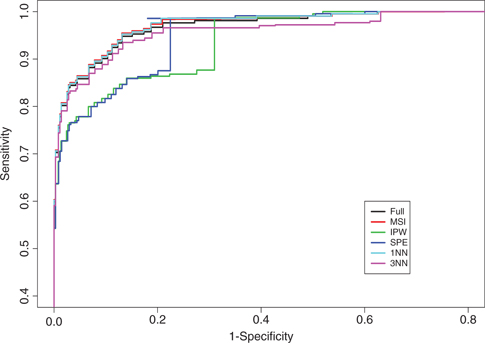
Illustrative example: estimated ROC curves of the test WR.

The obtained dataset shows a percentage of samples with true status known (verified) of about 58%. The percentage of benign samples is about 36% among verified samples and 99% among non-verified samples.

As traditional methods (MSI, IPW, SPE) require the use of parametric regression models for the conditional probability of a sample being malignant and/or selected (i.e., with the true status known), we use a generalized linear model for the status given WR and WCP with probit link to estimate the conditional disease probabilities, and a logistic regression model with WR and WCP as predictors to estimate the conditional selection probabilities. Clearly, this last model is misspecified.

Figure 1 shows the estimated ROC curves of the test WR obtained with the IPW, MSI, SPE, 1NN and 3NN methods. Such curves are benchmarked with the estimated ROC curve obtained from the complete dataset by using the Full estimator of sensitivity and specificity. The plot shows that the estimators MSI, 1NN and 3NN well behave, whereas the estimators IPW and SPE are highly biased. This could imply that, in our data, the probit model is a good approximation of the disease process, whereas misspecification of the selection model seems to highly affect the estimators IPW and SPE. This is somehow surprising, as far as the doubly robust SPE estimator is concerned, especially taking into account the good behavior of the MSI estimator. It is worth noting, however, that the SPE estimator produces estimates that are outside the range (0,1) and estimates of the specificity around 0.82 are not monotonically increasing for increasing values of the cutpoint c, as shown in Table 4, which reports estimates obtained for the sensitivity and the specificity at some values of c.

6 Variance estimation

In this section, we describe an approach to obtain estimates of the variances of the estimators proposed in Section 3. Such estimates could be used to build confidence intervals and perform hypothesis testing.

Recall that θˆ1 in (2) is the KNN imputation estimator of the disease prevalence θ1=Pr{D=1}, and that θˆ2 and θˆ3 are the KNN imputation estimators of θ2=Pr{T≥c,D=1} and θ3=Pr{T≥c,D=0}, respectively. Moreover, recall that Y=(T,X)⊤.

From Section 3, θˆ1 has asymptotic variance σ12=θ1(1−θ1)+ω12, where

This result follows by an application of Theorem 1 in Ning and Cheng [9]. Note that, in the expression of σ12, θ1(1−θ1) is the variance of D, and that the term ρ(Y)(1−ρ(Y) is the conditional variance of D given Y. Therefore, taking into account that I(T≥c)ρ(Y)(1−ρ(Y)) is the conditional variance of I(T≥c,D=1) given Y, the asymptotic variance of θˆ2 is given by σ22=θ2(1−θ2)+ω22, where

Similarly, for the asymptotic variance of θˆ3 one obtains σ32=θ3(1−θ3)+ω22.

Define γ1=Pr{T<c,D=1} and γ0=Pr{T<c,D=0}. Then, γ1=θ1−θ2 and γ0=1−θ1−θ3. Let

and

be the KNN imputation estimators of γ1 and γ0, respectively. Let ζ12 and ζ02 denote the asymptotic variances of γˆ1 and γˆ0, respectively. The above given arguments still hold, leading to the expressions ζ12=γ1(1−γ1)+ω32 and ζ02=γ0(1−γ0)+ω32, where

It is easy to see that γˆ1=θˆ1−θˆ2 and γˆ0=1−θˆ1−θˆ3. As a consequence, the asymptotic covariances between θˆ1 and θˆ2 – say σ12 – and θˆ1 and θˆ3 – say σ13 – may be obtained as σ12=(1/2)(σ12+σ22−ζ12) and σ13=(1/2)(σ12+σ32−ζ02).

Finally, recall that SeˆKNN(c)=θˆ2θˆ1 and SpˆKNN(c)=1−θˆ1−θˆ31−θˆ1. Therefore, by applying the delta method, one obtains

and

To obtain consistent estimates of the asymptotic variances given above, we may replace the unknown quantities in their expressions by the corresponding estimates. In particular, to estimate asVar(SeˆKNN(c)) and asVar(SpˆKNN(c)), we ultimately need the estimates θˆ1, θˆ2, θˆ3, ωˆ12, ωˆ22 and ωˆ32.

In a nonparametric regression imputation framework, quantities as ω12, ω22 and ω32 are typically estimated by their empirical counterparts. The propensity score π(y) is generally estimated by some kernel regression method (see Cheng [12]). In our context, however, we propose an approach that uses a nearest-neighbor rule to estimate both the functions ρ(y) and π(y) in ω12, ω22 and ω32. In particular, for the conditional probabilities of disease we can use the estimates ρ˜i=ρˆKˉi, for some suitable positive integer Kˉ. For the conditional probabilities of verification, instead, we choose the estimates π˜i=1Ki∗∑j=1Ki∗Vi(j), where {(Yi(j),Vi(j)),j=1,…,Ki∗} is a set of Ki∗ observed pairs, and Yi(j) denotes the jth nearest neighbor to Yi=(Ti,Xi)⊤among all Y’s. When π˜i is computed for a non-verified sample unit i, Ki∗ is set equal to the rank of the first verified nearest neighbor to the unit i, i.e., Ki∗ is such that Vi=Vi(1)=Vi(2)=⋯Vi(Ki∗−1)=0, and Vi(Ki∗)=1. When π˜i is computed for a verified sample unit i, Ki∗ is set equal to the rank of the first non-verified nearest neighbor to the unit i, i.e., Ki∗ is such that Vi=Vi(1)=Vi(2)=⋯Vi(Ki∗−1)=1, and Vi(Ki∗)=0. Observe that such procedure automatically avoids zero values for the π˜i’s. Then, based on the ρ˜i’s and the π˜i’s, we obtain the estimates