Void Formation during Diffusion – Two-Dimensional Approach

Introduction

The difference in diffusion coefficient of components causes several effects during mass transport process. Most often Kirkendall and Frenkel effects occur [1, 2]. Kirkendall effect (lattice drift) caused by the vacancy flux divergence leads to dislocation climb and subsequently to the construction of extra planes in accumulation region [3–5]. The drift velocity is then generated. This constraint means zero divergence of overall volume flux density:

When the only driving force is chemical potential gradient, μi=μich, the volume flux is given by

In this paper the generalized description of the interdiffusion in solid state will be shown. The final set of equations: mass and volume continuity; flux relation and vacancy evolution equation will be formulated. Moreover, the kinetic effects related to the difference of mobilities, namely the stress generation and relaxation [3, 6], vacancy migration and void formation will be discussed. Due to volume constraint, interdiffusion leads to the accumulation of matter, and thus this accumulation must be reduced to zero. This reduction will be realized by the introduction of (1) Kirkendall effect; (2) backstress effect and (3) non-equilibrium vacancy distribution (Frenkel effect). Void evolution during interdiffusion process in Fe-Pd system will be presented.

Mathematical formulation

Consider a multicomponent mixture, where ρi denotes the ith component density. The evolution of the density is described by the mass conservation law:

where Ji=ρivi denotes the overall flux of the ith component and vi is its volume velocity (the medium velocity). The overall fluxes and velocities of the mass in the mixture (alloy) are defined by the volume frame of reference:

where i = 1,…, r and r denotes the number of components. Nim=ρi/ρ is the molar fraction.

During an arbitrary transport process, when volume is affected by the distribution of every component mixture, the volume continuity equation [7] follows:

The final form of eq. (3) can be rewritten in the form that allows to determine the drift velocity:

In one-dimensional space the drift velocity can be expressed by analytical function (after integration):

However, in two or free dimension space eq. (4) should be solved by numerical method, e.g. by replacing the drift velocity by its potential, i.e. vdrift=grad udrift and then rewriting the second-order partial derivatives with second-order finite difference approximations. Thus, the Poisson equation is derived. Finally, the iterative update of the Jacobi iteration can be used.

The component flux, Ji≡ρivi, should be expressed by the proper constitutive formula. Moreover three additional effects should be introduced, mainly (1) Kirkendall, (2) backstress and (3) vacancy generation into the flux expression.

The Kirkendall effect means the movement of lattice from slower diffusant side towards the faster diffusant side with some drift velocity, vdrift. Thus this effect results in diffusion flux as follows:

The diffusion flux is defined by the Nernst–Planck flux equation [8, 9], which in general form reads:

where μi is the generalized diffusion potential of the ith component.

Backstress effect – the diffusion potential is affected by the internal stress effect – stress gradient appearing due to attempt of matter accumulation. Each diffusing atom of both species is affected by common stress force:

Non-equilibrium vacancy distribution – the diffusion potential is a difference of component chemical and common vacancy potentials, μi=μich−μV, and equalization of the diffusion fluxes instead of lattice shift is provided by the non-equilibrium vacancy gradient appearing due to attempt of matter accumulation. Role of effective force here is played by the gradient of vacancy chemical potential, proportional to the gradient of deviation of vacant sites fraction from its local equilibrium value:

Finally, the diffusion potential is a sum of component chemical, common vacancy and stress potentials, μi=μich+μV+μiInt, defined as follows:

The internal pressure, pInt, is a result of the difference in the diffusion coefficients of the components and difference in the lattice in diffusion couple (pressure generated by interdiffusion process):

The last equation defining the model is the vacancy exchange equation defined as

where Nv is the vacancy molar fraction, jv is the vacancy flux. Nveq and τv denote the vacancy equilibrium molar fraction and relaxation time, respectively.

To calculate void formation, in one-dimensional system, during the interdiffusion process one additional equation should be introduced, mainly, the void radii evolution [10, 11]:

where LV denotes the mean free path of vacancies and the vacancy diffusion coefficient is defined as DV=∑j,i=1j>irDiIDjINV∑i,j=1i≠jrDiINj.

Results

In this section the experimental and calculated results of interdiffusion and void formation will be shown. The calculations will be analysed in two-dimensional space. The simulation results will be verified with diffusion couple experiments in Fe-Pd binary system (Figure 1). The void radii will be estimated and the results for different calculation times will be presented. The following set of equations will be solved:

where gradμi=−kT1ρigradρi−kTρVeqgradρV−ρVeq. This set of equations will be supplemented with boundary conditions:

The subset ΩV denotes the position of the voids. The voids are initially introduced into the calculation mesh. Thus only the growth will be simulated. In two-dimensional space no additional equation for radii is needed.

Figure 1:

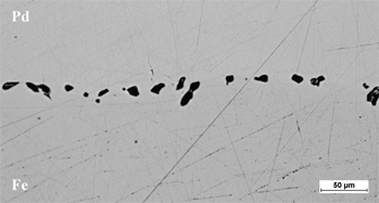
The experimental results of Frenkel effect (voids formation) during diffusion between pure Fe and Pd after 150 h at 1,273 K.

In Fe-Pb system the voids growth on the iron reach side of the diffusion couple. We assume that in Fe-Pd system the mean migration length for vacancy is LV=10−8m. The diffusion coefficient was calculated from Boltzmann-Matano analysis (from known experimental results of diffusion in Fe-Pd system at 1,273 K for 150 h – Figure 1). The results for different calculation times are shown in Figures 2– 5.

Figure 2:

The simulation results of the Fe concentration (a)–(b) and voids formation (vacancies evolution) (c)–(d) in Fe-Pd system after annealing at 1,273 K for 100 h.

Figure 3:

The simulation results of the Fe concentration (a)–(b) and voids formation (vacancies evolution) (c)–(d) in Fe-Pd system after annealing at 1,273 K for 200 h.

Figure 4:

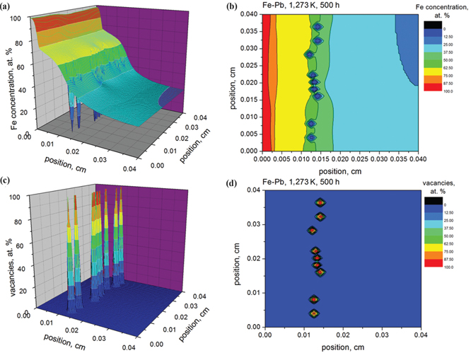
The simulation results of the Fe concentration (a)–(b) and voids formation (vacancies evolution) (c)–(d) in Fe-Pd system after annealing at 1,273 K for 500 h.

Figure 5:

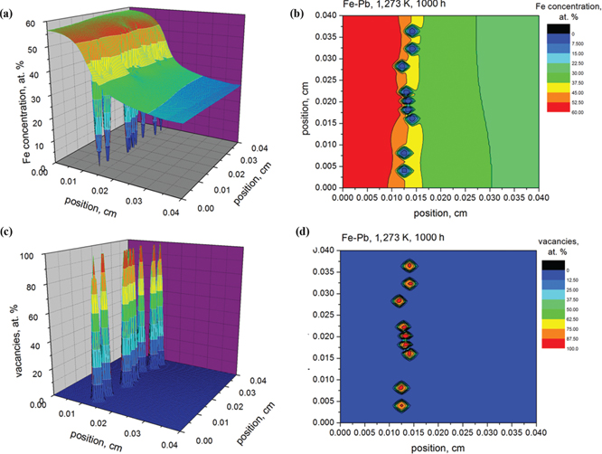
The simulation results of the Fe concentration (a)–(b) and voids formation (vacancies evolution) (c)–(d) in Fe-Pd system after annealing at 1,273 K for 1,000 h.

The estimated voids radii for different times are shown in Figure 6. It is clearly shown that the dependence is a parabolic one.

Figure 6:

The estimated void radii for different simulation time.

Conclusions

The presented method allowed the calculation of the interdiffusion process when Kirkendall, Frenkel and backstress effects are introduced. It was shown that the vacancy evolution in all diffusion calculations to approximate the real process should be introduced. The vacancies agglomerate in places where initially void was introduced as in real diffusion experiments. The results of the model were verified with experimental results for Fe-Pb binary system. Moreover, it was presented that the average radii of the void change parabolically with time. In the future the dynamics of the voids should be introduced, mainly simulation should take into account that the voids are moving during the diffusion process.

References

[1] Z. Grzesik and S. Mrowec, High Temp. Mater. Processes, 31 (2012) 539–551.10.1515/htmp-2012-0091Search in Google Scholar
[2] Z. Grzesik and M. Migdalska, High Temp. Mater. Processes, 30 (2011) 277–287.10.1515/htmp.2011.046Search in Google Scholar
[3] L. S. Darken, Trans. AIME., 174 (1948) 184–201.Search in Google Scholar
[4] A. D. Smigelskas and E. O. Kirkendall, Trans. AIME., 171 (1947) 130–142.Search in Google Scholar
[5] J. Bardeen and C. Herring, Diffusion in Alloys and the Kirkendall Effect in Imperfections in Nearly Perfect Crystals edited by W., Shockley, Wiley, New York (1952) 261–288.Search in Google Scholar
[6] R. W. Balluffi, S. M. Allen, W. C. Carter and R. A. Kemper, Kinetics of Materials, Wiley, New York (2005).10.1002/0471749311Search in Google Scholar
[7] B. Wierzba and M. Danielewski, Phys A., 390 (2011) 2325–2332.10.1016/j.physa.2011.02.047Search in Google Scholar
[8] W. Nernst, Z Phys Chem., 4 (1889) 129–181.10.1515/zpch-1889-0412Search in Google Scholar
[9] M. Planck, Ann Rev Phys Chem., 40 (1890) 561–576.10.1002/andp.18902760802Search in Google Scholar
[10] B. Wierzba, Phys A., 403 (2014) 29–34.10.1016/j.physa.2014.02.014Search in Google Scholar
[11] A. M. Gusak and N. V. Storozhuk, Phys. Metals Metall., 114 (2013) 197–206.10.1134/S0031918X13030071Search in Google Scholar
©2016 by De Gruyter
This article is distributed under the terms of the Creative Commons Attribution Non-Commercial License, which permits unrestricted non-commercial use, distribution, and reproduction in any medium, provided the original work is properly cited.
Articles in the same Issue
- Frontmatter
- Research Articles
- Effect of Activating Agent on the Preparation of Bamboo-Based High Surface Area Activated Carbon by Microwave Heating
- Research on the Microstructure and Mechanical Property of Ti-7Cu Alloy after Semi-Solid Forging
- Synthesis and Characterization of BiFeO3 Ceramic by Simple and Novel Methods
- Synthesis and Characterization of Lead Sulfide Nanostructures with Different Morphologies via Simple Hydrothermal Method
- Comparison of Brazed Residual Stress and Thermal Deformation between X-Type and Pyramidal Lattice Truss Sandwich Structure: Neutron Diffraction Measurement and Simulation Study
- Influence of V–N Microalloying on the High-Temperature Mechanical Behavior and Net Crack Defect of High Strength Weathering Steel
- Numerical Simulation on Optimization of Center Segregation for 50CrMo Structural Alloy Steel
- Direct Extraction of Ti and Ti Alloy from Ti-Bearing Dust Slag in Molten CaCl2
- Constitutive Equation for 3104 Alloy at High Temperatures in Consideration of Strain
- Microstructural Properties and Four-Point Bend Fatigue Behavior of Ti-6.5Al-2Zr-1Mo-1V Welded Joints by Electron Beam Welding
- Oxidizing Roasting Performances of Coke Fines Bearing Brazilian Specularite Pellets
- Purification of Niobium by Electron Beam Melting