Do political parties matter? Evidence from German municipalities
-
Nadine Riedel

 and
Christian Wittrock
and
Christian Wittrock

Abstract
We assess whether the partisanship of local councils affects the level and composition of local public spending by German municipalities. Our identification strategy exploits changes in the party with the absolute majority in the local council, combining an instrumental variable strategy with a matching approach to address potential selection into treatment. We find evidence for strong partisan effects: Communities with a left-wing council majority spend more on ‘people-oriented’ public goods and less on infrastructure than communities with a right-wing dominated council.
1 Introduction
Do political parties matter? That is, do they offer different policy platforms to voters and do they, once elected, implement different policies? Seminal models by Hotelling (1929) and Downs (1957) reject that notion and suggest that parties move to the center of the policy space and capture the median voter. Later work highlights that the median voter theorem relies on a set of non-trivial assumptions and shows that policy divergence may emerge under alternative assumptions (e. g. Wittman (1983) Calvert (1985), Cox and McCubbins (1986), Glaeser et al. (2005)). If politicians, for example, do not only care about being elected – as assumed in Downsian models – but also about implemented policies, parties cannot offer credible platforms that deviate from their representatives’ underlying policy preferences (Alesina (1988)).[1]
In this study, we empirically test for partisan effects on policy outcomes. The paper adds to the flourishing empirical literature on the topic 1) by assessing partisan effects on the local level (where existing work is still limited and result patterns tend to vary across studies, see below); 2) by relying on a rich dataset on local public spending that allows testing for partisan effects in detailed spending areas; 3) by proposing a new empirical strategy to identify partisan effects on the local level. Our findings point to strong partisan effects: Communities with a left-wing council majority tend to spend more on ‘people-oriented’ public goods and less on infrastructure than communities with a right-wing dominated council.
Our testing ground are German municipalities. In the main analysis, we assess whether the partisanship of local council majorities impacts on the level and composition of local public spending by German municipalities. For that purpose, we exploit detailed data on municipality spending across different spending categories between 1994 and 2006, including e. g. spending for child and youth care, culture and infrastructure. The data is linked to information on the party composition of local councils, which are the local legislative bodies that decide on local spending policies and taxes. To avoid that we confound partisan effects with differences between councils with absolute majorities and coalition majorities (e. g. reflecting common pool problems in council coalitions, see e. g. Persson et al. (2007), Meriläinen (2019)), we focus in the analysis on jurisdictions with a change in the party with the absolute majority in the local council.
Our empirical analysis is a fixed effect approach that compares changes in local spending policies when council majorities change from the main left-wing party SPD to the main right-wing party CDU/CSU or vice versa. To address potential selection into treatment, we rely on an instrumental variable (IV) strategy that exploits variation in party support at the federal level for empirical identification and draws on data from monthly opinion polls on intended voting behavior in federal elections (‘If next Sunday were to be a federal election day for the German national parliament, which party would you vote for?’). There are different potential shifters of intended voting behavior at the federal level, including changes in the perceived competence and popularity of party representatives at the national level (e. g., members of the national parliament or the national government) or perceived changes in their political positions. Exogenous events may also alter federal policy preferences; the ‘Fridays for Future’-protests, e. g., were associated with an increase in the support for the green party in Germany. Less than perfectly informed voters may rely on signals on party performance and party positions at the federal level – which are often more salient due to better media coverage – to proxy for expected party performance and positions at the local level; changes in federal party support may, therefore, trigger changes in local party support. Our empirical identification strategy exploits that in some jurisdictions these federal trends in party support imply that parties gain the majority of council seats, in others not. Common trends, like shifts in the general policy preferences of the electorate (that affect both, policy decisions at the federal and the local level irrespective of the party affiliation of decision makers) or common socio-economic shocks – are absorbed by (state-)year fixed effects in the estimation approach.
We, moreover, couple the instrumental variable strategy with an entropy matching approach (e. g. Hainmueller (2012)) to acknowledge that identification partly relies on differences in the initial vote shares for parties in council elections at the outset of our sample period. Specifically, we match localities with comparable spending patterns in the pre-election period and, on top of that, augment the empirical approach by a rich set of municipal-level control variables to ensure unbiased results.[2]
Our findings point to significant partisan effects. Specifically, a council seat majority of the main left-wing party SPD is associated with more spending for people-oriented public goods and less spending for infrastructure public goods relative to councils dominated by the main conservative party CDU/CSU. Quantitatively, the share of spending assigned to ‘people goods’ increases by 3.6 percentage points and the spending assigned to infrastructure goods drops by 7.2 percentage points respectively, which is quantitatively significant. Our results, in turn, reject partisan effects on tax setting behavior. In addition, we present a sensitivity analysis, where we use a RD design to assess whether the partisanship of municipalities’ mayors impacts local spending choices. Institutionally, mayors can influence policy outcomes by drafting and proposing legislation (which then has to be enacted by a simple majority of votes in the local council). Our RD design assesses whether spending policies systematically differ between municipalities where SPD mayoral candidates marginally won or marginally lost an election. The findings are broadly consistent with our baseline results: SPD mayors are found to spend more on ‘people-oriented’ goods and less on infrastructure.
Our paper contributes to a flourishing empirical literature on partisan effects. The more recent literature predominantly uses regression discontinuity designs for empirical identification (e. g. Lee et al. (2004), Ferreira and Gyourko (2009), Albouy (2013) and Curto-Grau et al. (2018)).[3] Our paper departs from this literature by using a different identification strategy, which arguably identifies partisan effects less locally than RD designs.[4]
Most of the existing work, moreover, tests for partisan effects on the national or state level (see e. g. Besley and Case (2003), Lee et al. (2004), Potrafke (2011a) and Potrafke (2011b)). Compared to this well-developed literature, analyses on the local level are still relatively limited – despite the fact that insights from higher federal tiers may not carry over to the local level, where interjurisdictional mobility is high and Tiebout sorting into homogenous local units or competition for mobile tax bases may limit the scope for partisan politics (e. g. Ferreira and Gyourko (2009)).[5] Existing work for the local level, moreover, largely focuses on the identification of partisan effects for policy outcomes other than government spending (see e. g. Sole-Olle and Viladecans-Marsal (2013), Folke (2014), Freier and Odendahl (2015)). Among those papers that consider public spending, most use total spending or broad spending categories (Pettersson-Lidbom (2008) and Ferreira and Gyourko (2009)) so that fine grained compositional spending changes are not observed. Our paper, in turn, is similar to Fiva et al. (2018) in that we can draw on detailed information on the level and composition of government expenditures. Our results show that the use of fine-grained spending data is essential: while we, similar to Ferreira and Gyourko (2009) and in contrast to Pettersson-Lidbom (2008), do not observe partisan effects in overall government spending, our findings point to partisan effects in detailed spending sub-categories, namely spending for social services and streets.
Most existing studies for the local level, moreover, either assess effects of mayoral partisanship on policy outcomes in the context of a majoritarian voting system (e. g. Ferreira and Gyourko (2009) and Gerber and Hopkins (2011)) or focus on the effect of political power of parties in the local council in the context of a proportional representation system (e. g. Folke (2014), Freier and Odendahl (2015), Fiva et al. (2018)). Our main analysis determines the effect of changing seat majorities for the main left-wing and right-wing party in German local councils, in turn. Note, moreover, that estimates for partisan effects at the local level display considerable heterogeneity. Ferreira and Gyourko (2009), for example, reject quantitatively significant partisan effects at the local level, while other work – including this paper – does find significant effects. This may reflect differences in the aggregation level of employed data (see above), but also differences in institutional contexts and testing grounds.[6]
The remainder of the article is as follows. Section 2 describes the institutional background and the data. The methodology is outlined in Section 3 and Section 4 presents the results. Finally, Section 5 concludes.
2 Institutional background and data
Our empirical analysis assesses the impact of partisanship of local council majorities on overall local spending and the composition of municipal spending using West German localities as a testing ground.[7] In the following, we describe the institutional background and the data set used for the empirical analysis.
2.1 Institutional background
According to the German constitution, German municipalities have elected legislative bodies and governments and have the right to solve any local matters autonomously (Article 28 of the German constitution). Localities generate income mainly from three sources. Firstly, a fraction of the personal income tax and the value added tax revenue administered at the federal and state level are distributed to German municipalities based on fiscal rules. Second, municipalities receive general and special grants by higher government tiers. Third, localities have two (major) own revenue instruments at hand: firstly, they autonomously set the local business tax rate, levied on business income earned within their borders and secondly, they choose the local property tax.[8] The majority of tax revenues from these two sources remains with the locality, only a minor fraction is redistributed by fiscal equalization schemes.[9] Note that the own tax revenue instruments generate a significant fraction of local income (on average about 20 %).[10]
German municipalities moreover provide various local public goods and services, e. g. related to the construction and maintenance of roads, sewerage, kindergartens and primary schools. Further, municipalities have to provide social benefits to the unemployed and social welfare recipients. Additionally, public goods and services related to culture and sport facilities, tourism, and public transport may be provided. While some expenditures are mandatory, including administration, social security and financing liabilities, others are optional, including e. g. spending for theaters, youth centers, the promotion of science, health care, sport and recreation facilities.
Finally note that legislative processes in the local councils are regulated in the municipal codes of the community’s hosting state, which are, however, highly similar across German states. Most importantly, in all federal states a simple majority of votes in the local council is required to enact changes in tax and spending policies.[11] On top of that, the mayor has some role in proposing and drafting legislations in all states, which implies that partisan effects may emerge with regard to the party composition of the local council as well as the party affiliation of the mayor. Our main analysis will assess the former; in robustness checks, we test for the latter. Note, moreover, that mayors are elected directly, with election dates varying across municipalities (also within a given state) and not being aligned with the election of local councils. Council elections are, in turn, synchronized for municipalities within the same state but vary between states. Table 1 depicts council election years for the West German states in our sample during our sample frame.
2.2 Data
As described above, the purpose of our analysis is to test for partisan effects on local government spending. Our analysis relies on rich data for spending of West German localities between 1992 and 2006, which is drawn from municipalities’ accounting information provided in the Jahresrechnungsstatistik. East Germany is disregarded as spending information is available from the late 1990ies onwards only. The spending data allows us to construct spending items for detailed and disaggregated expenditure categories. Note that, although German municipalities operate in a homogenous environment, their spending responsibilities are influenced by their size and status. To increase the comparability of our sample municipalities, we hence focus on small and mid-size cities with an average number of inhabitants over our sample period between 1,000 and 50,000 and also exclude urban cities (kreisfreie Staedte).
Elections for the Local Council by State and Year (1993 to 2006).
| Year | ||||||||||||||
| State | 93 | 94 | 95 | 96 | 97 | 98 | 99 | 00 | 01 | 02 | 03 | 04 | 05 | 06 |
| Schleswig-Holstein | ✓ | ✓ | ✓ | |||||||||||
| Lower Saxony | ✓ | ✓ | ✓ | |||||||||||
| North Rhine-Westphalia | ✓ | ✓ | ✓ | |||||||||||
| Hessia | ✓ | ✓ | ✓ | ✓ | ||||||||||
| Rhineland-Palatine | ✓ | ✓ | ✓ | |||||||||||
| Baden-Wuerttemberg | ✓ | ✓ | ✓ | |||||||||||
| Bavaria | ✓ | ✓ | ||||||||||||
| Saarland | ✓ | ✓ | ✓ | |||||||||||
Source: Own data collection.
We define different variables to capture the size and structure of municipality spending, namely (ln) overall real expenditures and (ln) financial expenditures as well as (ln) voluntary expenditures.[12] The voluntary spending measure accounts for the fact that communities have a number of mandatory spending obligations, which offer no room for partisan politics. The construction of the voluntary spending measure thus ignores expenditures that are organized and carried out by higher government tiers, for example, at the county level. Second, we exclude spending categories for which the voluntary dimension tends to be small. See Footnote 13 below for details on the specific spending categories that enter the voluntary spending variable.
To test for partisan effects on spending policies, we, in a first step, account for four relatively broad spending categories. These are (1) spending for general public goods, (2) spending for ‘people-oriented’ public goods, (3) spending for culture and (4) spending for infrastructure public goods. Each of the blocs, except of culture spending, consists of several subcategories. Spending for general public goods consists of spending for (1.1) public administration, (1.2) public safety and (1.3) commercial enterprises (e. g. own utility or public transport firms). Spending for people-oriented public goods consists of spending for (2.1) schools, (2.2) recreation (as parks and sport facilities) and (2.3) spending for people in need (social spending). Spending for infrastructure public goods consists of spending for (3.1) roads, (3.2) public facilities (e. g. sewerage, waste but also public markets) and (3.3) economic promotion.
Testing for partisan effects based on these broad categories offers the advantage, that estimates are expected to be more precise if the chosen subcategories are substitutes (what we presume). We will, however, in the following also test for partisan effects based on individual spending sub-categories. Note, moreover, that in defining these spending sub-categories, we focus on voluntary spending that local policymakers can plausibly control.[13]
See Tables 2 and 3 for descriptive statistics. On average municipalities have overall real expenditures of about 7.47 million Euro and financial expenditures of about 5.12 million Euro. The average share of voluntary expenditures to overall real expenditures is 42 %. General public spending, spending for ‘people-oriented’ goods and infrastructure spending make up broadly one third of overall spending each. Spending for cultural goods is, in turn, a small post in communities’ budget.
Descriptive Statistics for Overall Spending and Control Variables.
| Mean | Median | Std. Dev. | |
| Overall revenue in million Euro | 12.20 | 6.22 | 15.59 |
| Real expenditure in million Euro | 7.47 | 3.64 | 9.96 |
| Financial exp. in million Euro | 5.12 | 2.62 | 6.57 |
| Overall voluntary public good spending (as a fraction of overall spending) | 41.54 | 41.90 | 12.67 |
| Local business tax multiplier | 336 | 330 | 33 |
| Population in 1000 | 7.21 | 3.77 | 8.38 |
| Share population under 20 | 0.23 | 0.23 | 0.02 |
| Share population over 65 | 0.17 | 0.17 | 0.02 |
| Employees in 1000 | 2.31 | 1.23 | 2.66 |
| Unemployment rate (County) | 9.03 | 8.80 | 2.28 |
| Debt per capita | 929 | 920 | 300 |
Notes: The sample includes jurisdictions with two election periods, for which either there was an unchanged SPD or CDU majority in the local council or the council majority changed from SPD to CDU or from CDU to SPD. Overall there are 1364 observations with two-election periods (corresponding to 1058 unique municipalities). Some jurisdiction-election periods are included more than once (for example a jurisdiction with three election periods (SPD, SPD and CDU) is included with the election periods SPD-SPD and also with the two election periods SPD-CDU). Note that municipalities set a tax multiplier for the local business tax that is reported in the table. The tax burden is calculated as the product of this multiplier and a base rate (‘Messzahl’) that was 5 % for incorporated businesses during our sample period.
Source: Authors’ calculations based on Statistik Lokal and Jahresrechnungsstatistik 1994 to 2006.
Descriptive Statistics for Spending Composition.
| Mean expenditure shares for... | ...based on... | |
| as fraction of real overall spending in % | overall expenditures | voluntary expenditures |
| General public goods | 26.01 | 17.24 |
| Administration | 13.96 | 13.11 |
| Public safety | 4.49 | 4.13 |
| Commercial enterprises | 7.56 | 0.00 |
| ‘People-oriented’ public goods | 33.75 | 18.35 |
| Schools | 10.69 | 7.78 |
| Recreation | 5.57 | 4.00 |
| Social | 17.49 | 6.58 |
| Culture | 1.80 | 1.22 |
| Infrastructure public goods | 38.42 | 21.65 |
| Traffic | 18.10 | 15.46 |
| Public facilities | 17.93 | 4.45 |
| Economic promotion | 2.40 | 1.74 |
Notes: See the notes to Table 2 for the sample definition and the main text for the definition of the depicted variables.
Source: Authors’ calculations based on Statistik Lokal and Jahresrechnungsstatistik 1994 to 2006.
The sketched spending data is linked to information on the party composition of the local council obtained from the German Federal Statistical Offices. As will be presented in the next section, our empirical identification strategy relies on changes in the party composition of the local council in the wake of council elections. As indicated above, the timing of council election varies across German states (as does the term length, which varies between four and six years, see Table 1). On average, we observe three election periods per state within our data frame.
The party composition of local councils in Germany is shaped by the five main parties, that are also active at the state or federal level, as well as several civil parties that focus their activities to the local level. The five main parties are the Christian Democratic Union (CDU) and their Bavarian sister party the Christian Social Union (CSU) in the German state of Bavaria – in the following, we will refer to both as CDU-, the Free Democratic Party (FDP), the Social Democratic Party (SPD), the Greens (B90/Gruene) and the party ‘Die Linke’. Following Pappi and Eckstein (1998), these parties can be classified on a left-wing right-wing scale, where “Die Linke” is on the extreme left and the FDP on the extreme right. SPD and CDU are the moderate left and right-wing parties. The Greens are left to the SPD but are, additionally, proponents of environmentally-friendly policies. Note that this classification scheme cannot be used for the civil parties, whose programs tend to vary between localities.
To ferret out partisan effects, we will in the following concentrate the analysis on communities, where the local council is dominated by the large right-wing party, CDU, or the large left-wing party, SPD, in the observed election periods, or where there is a switch in the dominating party from SPD to CDU or from CDU to SPD. Note that with ‘dominated’, we mean that the considered party holds more than 50 % of the seats in the local council. This design helps us to, firstly, avoid effects related to divided governments and political coalitions and, secondly, does not require classifying local civil parties with varying political positions on the left-right-spectrum. Note, however, that this also implies that we disregard sample localities, where the local council is either dominated by a civil party or there is no dominant party at all. In the end, around 20 % of the West German municipalities (= 1058 jurisdictions) enter our sample. Around 75 % of the municipality-year observations are characterized by a local council that is dominated by the CDU and 25 % by a local council dominated by the SPD.
We further merged information on socio-economic characteristics of the localities to our data. These include overall population as well as the age structure of the population, number of employees, the unemployment rate and debt per capita (the latter two variables are available at the county level only). Descriptive statistics for the control variables for communities with an SPD or CDU dominated council respectively are shown in Table 2. The average municipality has around 7.200 inhabitants and around 23 % (17 %) of the population are aged below 20 (above 65).
3 Methodology
We draw on an instrumental variable strategy to assess the impact of partisanship of local council majorities on municipal spending choices. The second stage model reads
where
The vector
The empirical strategy hence resembles a difference-in-differences-design: We compare adjustments in the spending pattern of localities with changing council majorities in the course of local elections to localities where majorities remained constant. The key identifying assumption is that there is a common trend in the size and structure of local public spending of treatment and control communities and spending patterns would have developed similarly in the absence of the treatment. We cannot rule out that this assumption is violated: There may be confounding factors that correlate with treatment assignment and directly impact the dependent variable. If municipalities, for example, face adverse economic shocks or threats of future adverse economic shocks (e. g. important local employers considering relocation), the electorate might push for adjustments in public spending (e. g. increases in social spending and adjustments in investment spending) and, simultaneously, give their vote to the conservative CDU/CSU at increased rates, which are commonly perceived to have more economic competence among their ranks (see e. g. Infratest-dimap (2019)). While actual changes in economic conditions can be absorbed by observed control variables (e. g. the local unemployment rate), signals of future shocks (e. g. considerations about plant relocation of large local employers) may act as a confounder and are genuinely unobserved.
We hedge against this threat by augmenting the fixed effect strategy with an instrumental variable approach. The IV strategy exploits variation in party votes at the local level induced by changing party support at the federal level, drawing on data from monthly opinion polls on intended voting behavior prepared by the ‘Forschungsgruppe Wahlen’ – a scientific society – for one of the two main public television channels in Germany. The poll is based on a representative sample of the German population eligible to vote. Specifically, we use poll results for the following question: “If next Sunday were to be a federal election day for the German national parliament, which party would you vote for?”. There are different potential shifters of intended voting behavior at the federal level, including changes in the perceived competence and popularity of party representatives at the national level (e. g., members of the national parliament or the national government) or perceived changes in their political positions. Exogenous events may also alter federal policy preferences; the ‘Fridays for Future’-protests, e. g., were associated with an increase in the support for the green party in Germany. Less than perfectly informed voters may rely on signals on party performance and party positions at the federal level – which are often more salient due to better media coverage – to proxy for expected party performance and positions at the local level; changes in federal party support may, therefore, trigger changes in local party support. Our empirical identification strategy exploits that in some jurisdictions these federal trends in party support imply that parties gain the majority of council seats, in others not. Common trends in policy outcomes, for example related to shifts in the general policy preferences of the electorate are absorbed by (state-)year fixed effects.
Technically, the instrument is constructed as follows: For municipalities with a SPD majority in the local council in the first election period, we predict the seat share of the main contending party – the CDU – in the following election
The variation is thus allocated to two instruments:
In terms of intuition, using
We consider this assumption to hold. First note that the difference-in-differences nature of the setup implies that we absorb common changes in underlying policy preferences (that may affect both, policy decisions at the federal and the local level irrespective of the party affiliation of decision makers) as they impact policy outcomes in the treatment group and control group alike. We, in turn, exploit that federal trends in party support imply that parties gain the majority of council seats in some municipalities, but not in others (depending on the initial seat shares in the prior election, see below). Second, the fact that we use shocks to voting intentions rather than actual changes in electoral outcomes at the federal level hedges us against concerns that shifts in federal party support may reallocate resources from politically unaligned to politically aligned municipalities, thereby affecting local budgetary outcomes. To further hedge against this concern, we, moreover, control for federal grants received by localities from higher government tiers in the estimation strategy.
A third concern arises because treatment assignment may correlate with a party’s seat share at t: To see this, consider again the example sketched above: If, in the construction of
The IV strategy is therefore only valid if the initial seat share for SPD or CDU does not affect changes in overall spending and spending composition.[15] As we cannot rule out such a correlation, we combine our difference-in-differences-IV strategy with a matching approach. The underlying idea is to draw on observed changes in spending patterns in the pre-election period and to re-weight treatment group and control group such that pre-election (and thus plausibly common) trends in public spending are similar in the two groups. While our main concern is that differences in initial seat shares (an observed variable) may lead to different underlying spending trends, matching on pre-trends would also account for other – observed and unobserved – reasons why underlying trends in the dependent variable may differ between the treatment and control group.[16] Note in this context that, while the number of treated municipalities is rather small, the matching analysis draws on a large pool of control jurisdictions with unchanged council majorities.
The most often used matching approach in the literature is propensity score matching (where the propensity score represents the likelihood of being treated). It can be used to match observations, e. g. to find the closest control unit for every treatment observation, or to weight observations to create balance between control and treatment units (see Imbens2004: for a review). One particular assumption of the propensity score approach – in addition to conditional independence – is that the distribution behind the mean of the matching variables is the same, as otherwise observed differences between treatment and control group remain unaccounted and bias the estimated average treatment effect.
One recently proposed approach to overcome the lack of co-variante balancing in a selection-on-observables framework is entropy-balancing (Hainmueller (2012)). The main advantage of this method is that covariate balancing is not just assumed but enforced in a constrained, nonlinear estimation approach. The approach obtains weights for each targeted moment of the balancing/matching variables for treatment and control group subject to the balancing constraints. The resulting weights can then be used in a weighted regression.[17]
Therefore, we apply entropy balancing to balance spending patterns of treatment and control jurisdictions in the year before the election (but will show that using propensity score matching yields similar results to the ones presented in our main model). As our analysis separately assesses adjustments in local spending in the wake of changes in council-majorities from SPD to CDU and vice versa (see above) – and underlying spending trends may differ for localities where council majorities switch from SPD to CDU and those where council majorities switch from CDU to SPD-, we create two subsamples. Each of the two subsamples includes two consecutive election periods of jurisdictions. In the first subsample (Panel A), we include two types of jurisdictions: (i) jurisdictions which had a CDU majority in both election periods and (ii) jurisdictions which had a CDU majority in the first election period and a SPD majority in the second election period. In the second subsample (Panel B), we include (i) jurisdictions with a SPD majority in the local council in both election periods and (ii) jurisdictions with a SPD majority in the first election period and a CDU majority in the second election period.[18]
We use the same set of matching variables for both subsamples. Specifically, we include the two year change in (ln) real expenditures, (ln) financial expenditures and the local business tax rate as well as the voluntary spending shares for general public goods, people public goods, culture and infrastructure public goods in the year prior to the second-period election. Further, we match on state dummies. We target for all variables (except for the state dummies) mean and variance of the distribution. The resulting balancing statistics for Panel A and Panel B are shown in Table A1 and Table A2 in the Appendix. The descriptive statistics as well as the point estimates for the treatment indicator obtained when regressing the matching variables on the treatment variable suggests that the entropy balancing is highly effective as all variables in the re-weighted sample are very similarly distributed for treatment and control group. Please note that we do not match on other jurisdiction characteristics as we control for them in the regressions. In particular, in our baseline approach we do not match on the levels of the matching variables as we include in all estimations municipality fixed effects. We address this, however, in a robustness check. Combining both subsamples gives us our final estimation sample, which includes 1,364 two-election periods (or 1,058 unique jurisdictions) and 12,702 municipality-year observations.
4 Results
Table 4 reports our baseline findings. Row (1) shows the results of our preferred estimation strategy, which is the instrumental variable approach using the entropy-balanced sample. The dependent variables are the log of municipalities’ overall real expenditures, financial expenditures, voluntary expenditures and localities’ spending composition as captured by voluntary spending shares for general expenditures, ‘people-oriented’ expenditures, cultural expenditures and infrastructure spending. The main explanatory variable is a dummy variable indicating that the SPD holds the majority of council seats, instrumented as described in the previous section. The sample accounts for all communities in our data, i. e. those that experienced a switch from SPD to CDU and those that experienced a switch from CDU to SPD (as well as the control municipalities, where majorities did not change).
The F-statistic for the first stage is around 15 and thus suggests that our instruments are relevant. Moreover, the first stage point estimates are as expected (the coefficient estimate for the instrument predicting switches from a CDU to a SPD majority is 0.57 (se: 0.32) and the coefficient estimate for the instrument predicting a switch from a SPD to a CDU majority is −0.63*** (se: 0.13)). See the first stage results reported in Column (1) of Table A5 in the Appendix.
Estimation Results – Overall Spending and Shares for Voluntary Spending.
| Dep. Var. | (ln) | (ln) | (ln) | Local | Share | |||
| Real Exp. | Financial Exp. | Voluntary Exp. | Business Tax Rate | General Exp. | People Exp. | Culture Exp. | Infrastructure Exp. | |
| (1) | (2) | (3) | (4) | (5) | (6) | (7) | (8) | |
| IV & Weighted Sample: N = 12,702, F-Statistic First Stage: 15.67 | ||||||||
| SPD | −0.0818 | −0.0880 | −0.1620* | 2.3852 | 0.5303 | 3.5948** | 0.2521 | −7.2824*** |
| (0.0996) | (0.1522) | (0.0856) | (2.3891) | (1.2264) | (1.3525) | (0.1764) | (1.8848) | |
| Hansen | 0.126 | 0.160 | 0.306 | 0.469 | 0.983 | 0.674 | 0.401 | 0.924 |
| Reduced Form & Weighted Sample: Panel A (CDU-CDU/SPD) N = 9,451 | ||||||||
| Instrument CDU-SPD | 0.0628* | 0.1395** | −0.0532 | 0.6607 | 0.6593 | 3.5621** | 0.0640 | −4.4167** |
| (0.0328) | (0.0601) | (0.0502) | (2.7898) | (1.1356) | (1.1274) | (0.1539) | (1.6737) | |
| Reduced Form & Weighted Sample: Panel B (SPD-SPD/CDU), N = 3,251 | ||||||||
| Instrument SPD-CDU | 0.1090 | 0.1397 | 0.1242** | −0.8767 | −0.4825 | −2.0076* | −0.1936 | 4.2456*** |
| (0.0620) | (0.0972) | (0.0538) | (1.4617) | (0.8062) | (0.9810) | (0.1237) | (1.0832) | |
| Control Var | ✓ | ✓ | ✓ | ✓ | ✓ | ✓ | ✓ | ✓ |
| Municipality FE | ✓ | ✓ | ✓ | ✓ | ✓ | ✓ | ✓ | ✓ |
| State-Year FE | ✓ | ✓ | ✓ | ✓ | ✓ | ✓ | ✓ | ✓ |
Notes: All regression include control variables, municipality fixed effect as well as state-year fixed effects. The dependent variables are: (ln) of municipalities’ real spending (Column (1)), (ln) of municipalities’ financial spending (Column (2)), (ln) of municipalities’ voluntary spending (Column (3)), jurisdictions’ business tax rate choice (Column (4)) and the voluntary spending shares for general public goods (Column (5)), people public goods (Column (6)), culture (Column (7)) and infrastructure public goods (Column (8)). Row (1) shows the second stage estimate for a dummy variable indicating an SPD-dominated local council when using the instrumental variable strategy described in the main text and assuming symmetry of effects when localities change from SPD to CDU or vice versa. Row (2) shows the results of the reduced form estimates in the subsample of Panel A (localities that switch from a CDU to a SPD majority or experience an unchanged CDU majority) using only the instrument that predicts whether the SPD – as the contending party – gains the majority of council votes. Analogously, Row (3) shows results of reduced for estimates in the subsample of Panel B (localities that switch from a SPD to a CDU majority or experience an unchanged SPD majority) using only the instrument that predicts whether the CDU – as the contending party – gains the majority of council votes. For all specifications, we use entropy-balanced samples. Standard errors in parenthesis are robust and clustered at the municipality level and for election periods. *, **, and *** denote significance at the 10, 5, and 1 % level.
Source: Authors’ calculations based on Statistik Lokal and Jahresrechnungsstatistik 1994 to 2006.
The results suggest no impact of the partisanship of local council majorities on a jurisdiction’s local business tax rate choice, general spending or spending for culture. SPD majorities are, however, observed to devote a higher share of overall voluntary spending to people public goods and less to infrastructure public goods. The effect sizes are with 3.6 and −7.2 percentage points substantial given that the mean spending share of the respective categories is around 18 % and 22 % respectively. Our result, furthermore, suggest that SPD majorities engage in lower voluntary spending (as categorized by us). This could explain why the reduction of infrastructure expenditures is larger than the increase in people-oriented expenditures.
Furthermore note that, given that we have two instruments, one for the change from CDU to SPD majorities and one for the change from SPD to CDU majorities, we are able to assess directly whether the observed policy responses are symmetric and hence reflect partisan behavior (i. e. wether we find similar coefficient estimates for
This finding is corroborated when we reestimate the model in a subsample of localities that either switch from a CDU to a SPD majority or have an unchanged CDU council majority, denoted as ‘Panel A’ in Row (2) of Table 4, and a subsample of localities that either switch from a SPD to a CDU majority or have an unchanged SPD council majority, denoted as ‘Panel B’ in Row (3) of Table 4. As the first stage F-statistic is below 10 in these subsample models, we report the results of reduced form estimates, where we regress policy outcomes on the excluded instrument respectively.[20] The result pattern resembles our baseline findings. Importantly, the point estimate for people-oriented and infrastructure spending have the opposite signs and are statistically significant in both subsamples, suggesting that the identified policy adjustments reflect partisan effects rather than behavioral adjustments to gaining legislative power.
To assess whether endogeneity of some of our control variables may act as a confounder, Row (1) in Table A6 in the Appendix reports the results when excluding our set of control variables. This leaves the result pattern largely unchanged.[21] The effect size is slightly reduced but the estimates are within the confidence intervals of our baseline results. In Row (2), results are reported when estimating not on the municipality-year level but when collapsing the data on the municipality-election term level. Results are very similar. Moreover, we assess whether estimates change when we not only match on changes in pre-election spending but also on the levels. Since the matching does not converge when matching is in addition on state-indicators, Row (3) in Table A6 shows the results when matching only on changes in pre-election spending patterns but not on state-indicators. The precision of the estimates is reduced and the effect sizes are somewhat larger but again within the confidence intervals of our baseline results.[22] Row (4) then shows the results when matching on levels as well as changes in pre-election spending. The balancing statistics suggest again a successful strategy (see Table A3 and Table A4). The results are very similar to the ones in Row (3), suggesting that the municipality fixed effects absorb level differences in the baseline model.[23] In the last row of Table A6, we, moreover, rerun our baseline model using standard propensity score matching rather than entropy matching, which yields qualitatively and quantitatively unchanged results.
Table 5 further refines the analysis and assesses which subcategories within the broader categories of ‘people-oriented’ spending and infrastructure spending are driving the results. Increased ‘people-oriented’ spending under SPD-dominated local councils is suggested to particularly reflect higher social spending (around 50 %) and higher spending for recreational goods (35 %), while lower infrastructure expenditures is suggested to particularly reflect lower spending for streets (90 %) and lower spending for economic promotion (10 %). Note that the Hansen tests again support the notion that the observed differences reflect partisan behavior (as symmetric effects of SPD-majorities are observed when identification relies on changes from SPD to CDU majorities and vice versa). Reduced form estimates in the subsamples of Panel A and B largely confirm these findings (see Rows (2) and (3) of Table 5).
Estimation Results – Shares for Voluntary Spending in Subcategories.
| Dep. Var. | Expenditure Shares | |||||
| ‘People-Oriented’ Exp. | Infrastructure Exp. | |||||
| Schools | Recreation | Social | Streets | Public Facilities | Economic Promotion | |
| (1) | (2) | (3) | (4) | (5) | (6) | |
| IV & Weighted Sample: N = 12,702, F-Statistic First Stage: 15.67 | ||||||
| SPD | 0.5260 | 1.3130 | 1.7558** | −6.8670*** | 0.3679 | −0.7834* |
| (1.1192) | (0.9962) | (0.6230) | (1.9743) | (0.8119) | (0.4255) | |
| Hansen | 0.480 | 0.618 | 0.714 | 0.687 | 0.653 | 0.670 |
| Reduced Form & Weighted Sample: Panel A (CDU-CDU/SPD), N = 9,451 | ||||||
| CDU-SPD | 1.4332 | 0.6423 | 1.4866 | −5.4865*** | 2.1657 | −1.0959** |
| Instrument | (0.8838) | (0.5080) | (0.9975) | (1.3483) | (1.2694) | (0.4782) |
| Reduced Form & Weighted Sample: Panel B (SPD-SPD/CDU), N = 3,251 | ||||||
| SPD-CDU | −0.1037 | −0.8712 | −1.0328** | 3.6361** | −0.0783 | 0.6878* |
| Instrument | (0.8702) | (0.8942) | (0.3817) | (1.0847) | (0.4787) | (0.3204) |
| Control Var | ✓ | ✓ | ✓ | ✓ | ✓ | ✓ |
| Municipality FE | ✓ | ✓ | ✓ | ✓ | ✓ | ✓ |
| State-Year FE | ✓ | ✓ | ✓ | ✓ | ✓ | ✓ |
Notes: All regression include control variables, municipality fixed effect as well as state-year fixed effects. The dependent variables are: the municipalities’ voluntary spending shares for schools (Column (1)), recreation (Column (2)), social services (Column (3)), streets (Column (4)), public facilities (Column (5)) and economic promotion (Column (6)). The structure of the table follows Table 4 (instrumental variable estimates in Row (1) and reduced form estimates in Row (2) and (3), see the notes to Table 4).For all specifications, we use entropy-balanced samples. Standard errors in parenthesis are robust and clustered at the municipality level and for election periods. *, **, and *** denote significance at the 10, 5, and 1 % level.
Source: Authors’ calculations based on Statistik Lokal and Jahresrechnungsstatistik 1994 to 2006.
Finally, Table 6 intends to refine the interpretation of our results. Specifically, our main findings suggest that spending shares for infrastructure drop under SPD-dominated local councils, while spending shares for people-oriented public goods increase; in quantitative terms, the decline in infrastructure spending, however, appears to outweigh the increase in people-oriented expenditures. The baseline table already suggests that this pattern is matched by a drop in overall voluntary spending under SPD-dominated councils. On top of that, we cannot exclude that spending in other categories, namely voluntary general spending, may also increase with SPD-dominated local councils – albeit the positive coefficient estimate for the SPD dummy does not gain statistical significance in the latter instance.[24] The results in Column (1) of Table 6, moreover, suggest that the share of voluntary and mandatory expenditures assigned to the general spending category is higher in municipalities with SPD-dominated local councils. Within this category, adjustments in administration and public safety expenditure explain around one third of this response and adjustments in public company expenditures explain the remaining two thirds (cf. Columns (2) and (3)). Reduced form estimates in the subsamples of Panel A and Panel B (Rows (2) and (3)) confirm these findings. This suggests that some of the general expenditure categories that we assigned to mandatory spending are influenced by local partisan politics.
Estimation Results – Mandatory and Voluntary General Spending.
| Dep. Var. | Share | ||
| General Exp. | Admin. Exp. | Public Firms Exp. | |
| (1) | (2) | (3) | |
| IV & Weighted Sample: N = 12,702, F-Statistic First Stage: 15.67 | |||
| SPD | 3.4082** | 0.9341 | 2.4741* |
| (1.1024) | (1.2954) | (1.1927) | |
| Hansen | 0.307 | 0.809 | 0.204 |
| Reduced Form & Weighted Sample: Panel A (CDU-CDU/SPD), N = 9,451 | |||
| CDU-SPD | 2.7949* | 0.7016 | 2.0933** |
| Instrument | (1.4867) | (1.1717) | (0.8640) |
| Reduced Form & Weighted Sample: Panel B (SPD-SPD/CDU), N = 3,251 | |||
| SPD-CDU | −1.8818** | −0.8833 | −0.9985 |
| Instrument | (0.7276) | (0.8340) | (0.8116) |
| Control Var | ✓ | ✓ | ✓ |
| Municipality FE | ✓ | ✓ | ✓ |
| State-Year FE | ✓ | ✓ | ✓ |
Notes: All regression include control variables, municipality fixed effect as well as state-year fixed effects. The dependent variables are: the municipalities’ expenditures share for mandatory and voluntary general public goods (Column (1)), administration and security (Column (2)) and public companies (Column (3)). The structure of the table follows Table 4 (instrumental variable estimates in Row (1) and reduced form estimates in Row (2) and (3), see the notes to Table 4). For all specifications, we use entropy-balanced samples. Standard errors in parenthesis are robust and clustered at the municipality level and for election periods. *, **, and *** denote significance at the 10, 5, and 1 % level.
Source: Authors’ calculations based on Statistik Lokal and Jahresrechnungsstatistik 1994 to 2006.
Finally, we assessed the robustness of our findings to using an RD methodology. To do so, we draw on data provided by Freier and Odendahl (2015) for two German states, Bavaria and North-Rhine-Westpfalia, and use an RDD to determine whether the partisanship of the mayor impacts on local spending patterns.[25]
Mayors in German municipalities can influence policy outcomes by proposing and drafting legislation (which then needs to be enacted by a majority vote of the local council). In both considered states, the mayor is directly elected with an absolute majority of votes. If no candidate wins the absolute majority, run-off elections take place. Since focusing only on run-off elections could introduce a selection bias, we account for all (final) elections and the victory margin of SPD and CDU mayor candidates.[26] We run two sets of models: one comparing the spending policies of localities with SPD mayors to that of communities with mayors from all other parties/mayors without party affiliation and one comparing spending policies of communities with CDU mayors to those with mayors from all other parities/mayors without party affiliation. Focusing on races between SPD and CDU candidates alone would strongly reduce our sample size as candidates from other parties and independent candidates often run for office. In the RD strategy, we thus test for partisan effects asking whether SPD mayors and CDU mayors respectively implement systematically different spending policies than mayors from other parties/mayors without party affiliation.
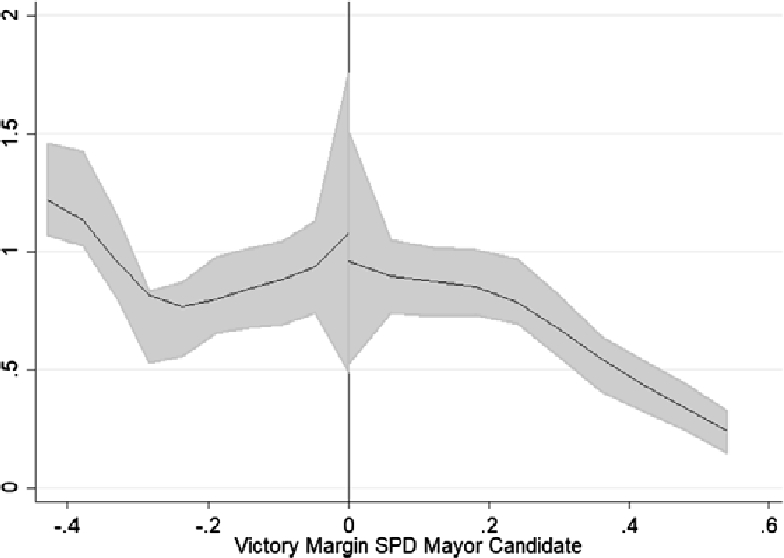
Victory Margin SPD Candidates.
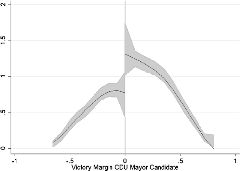
Victory Margin CDU Candidates.
One important requirement for a valid RDD is no manipulation/sorting at the threshold (McCrary (2008)). We assess this assumption by using the approach outlined by Cattaneo et al. (2019) and find no sorting when comparing races marginally won and lost by SPD candidates. When comparing races marginally won and lost by CDU candidates, there is evidence for sorting around the threshold (SPD candidates: p-value: 0.80 and CDU candidates: p-value 0.01, see also Figures 1 and 2).[27] We thus in the following focus on the races marginally won and lost by SPD candidates.
The base results are reported in Table 7 and compare spending outcomes in jurisdictions with and without SPD mayors. We choose the victory margin using the RD bandwidth window selection framework developed by Cattaneo et al. (2014) and our set of municipality control variables as well as all pre-determined outcome variables. This test recommends a victory margin of 1.9 % based on a minimum p-value for the covariance balance test of 0.1. This leaves us with 36 observations.
RD Results (Victory Margin: 1.9 %).
| Dep. Var. | (ln) | (ln) | (ln) | Local | Share | |||
| Real Exp. | Financial Exp. | Voluntary Exp. | Business Tax Rate | General Exp. | People Exp. | Culture Exp. | Infra. Exp. | |
| (1) | (2) | (3) | (4) | (5) | (6) | (7) | (8) | |
| Panel 1: Current Election Period (N = 36) | ||||||||
| SPD | 0.2630 | 0.1647 | 0.3475 | 9.8278 | 1.0738 | 3.1196 | 0.7112 | −2.9138 |
| (0.2753) | (0.2704) | (0.2847) | (13.0205) | (1.7407) | (2.0729) | (0.5540) | (2.1391) | |
| Panel 2: Current Election Period, Controlling for Lagged Dependent Variable (LDV) (N = 36) | ||||||||
| SPD | 0.0482 | 0.0365 | 0.0640 | −6.9625* | 1.4289 | 1.8403 | 0.0299 | −3.0466* |
| (0.0437) | (0.0732) | (0.0625) | (3.7489) | (0.8945) | (1.2819) | (0.4325) | (1.7404) | |
Notes: The table shows the point estimates for the SPD mayor indicator variable using a regression discontinuity design with a 1.9 % victory margin. The dependent variables are: (ln) real spending (Column (1)), (ln) financial spending (Column (2)), (ln) voluntary spending (Column (3)), jurisdictions’ business tax rate multiplier (Column (4)) and the voluntary spending shares for general public goods (Column (5)), people public goods (Column (6)), culture (Column (7)) and infrastructure public goods (Column (8)). In Panel 2, we control for the lagged dependent variable. Standard errors in parenthesis. *, **, and *** denote significance at the 10, 5, and 1 % level.
Source: Authors’ calculations based on Statistik Lokal and Jahresrechnungsstatistik 1994 to 2006.
Panel 1 of Table 7 reports the base estimate. The result pattern resembles our baseline findings: SPD mayors tend to engage in less infrastructure spending and more spending on people-goods than mayors from other parties/with no party affiliation. The estimates are relatively imprecise, however, and none of the estimated coefficients gains statistical significance. To improve efficiency, Panel 2 reestimates the baseline model controlling for the lagged dependent variable.[28] In this specification, the coefficient estimate for infrastructure spending turns out marginally significant, suggesting that SPD mayors allocate less resources to infrastructure investments.[29] Appendix B, moreover, presents numerous robustness checks, including placebo tests, checks for the distribution of observed characteristics left and right of the threshold, robustness tests where we adjust the bandwidth of the RD model and specifications, where we opt for a more flexible modeling of the forcing variable. We, moreover, present results based on the recently proposed bias corrected local polynomial RD estimator (Calonico et al. (2014)) which has been found to be closest to experimental estimates (Hyytinen et al. (2018)). From our perspective, the RD analysis offers two insights: First, the, in part, failed specification tests suggest that RD design is not an ideal approach to identify partisan effects in our empirical context as we cannot rule out sorting at the threshold (see Figure 2). This supports our decision to opt for a different identification approach in our main analysis. Second, we, nevertheless, consider it reassuring that the RD model in the sub-analyses for the SPD mayoral candidates – where specification tests are passed – yields results that are similar to our base analysis.
5 Conclusion
The aim of this paper was to assess the role of partisanship of West German local council majorities on the size and composition of local public spending. We combine a instrumental variable fixed effect regression approach with an entropy balanced matching strategy to empirically identify the effect of interest. The results point to stark partisan effects: SPD council majorities are found to spend more on people-oriented public goods and less on infrastructure public goods. The driving subcategories are spending for recreation and social spending on the one hand and spending for streets and economic promotion on the other.
Funding source: Deutsche Forschungsgemeinschaft
Award Identifier / Grant number: SI 2050/1-1
Award Identifier / Grant number: RI 2491/2-1
Funding statement: We gratefully acknowledge financial support from the German Research Foundation (Simmler: SI 2050/1-1 and Riedel: RI 2491/2-1).
Acknowledgment
We are grateful to participants of the Congress of the German Economic Association in Vienna and of the Annual Conference of the International Institute of Public Finance in Tokyo for helpful comments and suggestions.
Appendix A Additional descriptive statistics and estimation results for main approach (IV)
Descriptive Statistics for Panel A (CDU-CDU/SPD): Unweighted and Entropy-Balanced (Baseline).
| First Election Period Variables | Control CDU-CDU | Treatment CDU-SPD | Point Estimate [p-value] Treatment in a Regression with | |||||
| Unweighted | Entropy-Balanced | |||||||
| Mean | Variance | Mean | Variance | Mean | Variance | No controls | State-Year FE | |
| Δ Local business tax multiplier | 5.81 | 113.06 | 3.02 | 27.89 | 3.05 | 26.70 | 0.03 [0.98] | 0.21 [0.87] |
| Δ (ln) Real expenditures | 0.02 | 0.04 | 0.10 | 0.04 | 0.10 | 0.04 | 0.01 [0.93] | 0.02 [0.73] |
| Δ (ln) Financial expenditures | 0.03 | 0.07 | 0.12 | 0.04 | 0.12 | 0.04 | 0.00 [0.93] | 0.01 [0.80] |
| Voluntary expenditure shares for | ||||||||
| Δ General public goods | 0.37 | 28.21 | −2.95 | 35.85 | −3.03 | 33.11 | −0.08 [0.96] | −0.15 [0.92] |
| Δ People public goods | 0.21 | 61.58 | 0.62 | 56.05 | 0.59 | 53.40 | −0.03 [0.98] | 0.01 [0.99] |
| Δ Culture | −0.02 | 3.54 | 0.01 | 0.65 | −0.01 | 0.60 | −0.02 [0.92] | −0.05 [0.82] |
| Δ Infrastructure public goods | 0.19 | 92.97 | 3.00 | 88.69 | 2.85 | 85.62 | −0.15 [0.94] | −0.43 [0.84] |
| Jurisdictions | 1006 | 1006 | 15 | 1021 | 1021 | |||
| Jurisdiction-Year-Observations | 9310 | 9310 | 141 | 9451 | 9451 | |||
Notes: The table reports descriptive statistics for jurisdictions with CDU dominated councils that changed to a SPD dominated council (treatment group) and jurisdictions with CDU dominated councils with no change in the majority in the local council, before entropy-balancing (unweighted) and after. The matching variables are the two year changes of (ln) real expenditures, (ln) financial expenditures and the local business tax multiplier as well as the spending share for general, people, culture and infrastructure public goods in the last year before the election as well as state indicators. The last two columns show the point estimate [p-value] for a treatment dummy in regressions of the matching variable on the treatment indicator without control variables and with state-year fixed effects respectively, in the matched sample.
Descriptive Statistics for Panel B (SPD-SPD/CDU): Unweighted and Entropy-Balanced (Baseline).
| First Election Period Variables | Control SPD-SPD | Treatment SPD-CDU | Point Estimate [p-value] Treatment in a Regression with | |||||
| Unweighted | Entropy-Balanced | |||||||
| Mean | Variance | Mean | Variance | Mean | Variance | No controls | State-Year FE | |
| Δ Local business tax multiplier | 2.14 | 38.77 | 4.01 | 55.52 | 4.21 | 58.58 | 0.20 [0.89] | 0.16 [0.92] |
| Δ (ln) Real expenditures | 0.03 | 0.03 | 0.01 | 0.03 | 0.01 | 0.03 | −0.01 [0.85] | −0.01 [0.84] |
| Δ (ln) Financial expenditures | 0.05 | 0.08 | 0.05 | 0.09 | 0.03 | 0.08 | −0.02 [0.82] | −0.02 [0.82] |
| Voluntary expenditure shares for | ||||||||
| Δ General public goods | 0.72 | 22.01 | −0.14 | 12.56 | −0.19 | 12.29 | −0.05 [0.94] | −0.00 [0.99] |
| Δ People public goods | 0.60 | 40.42 | 1.90 | 59.57 | 1.90 | 59.84 | 0.00 [0.99] | −0.02 [0.99] |
| Δ Culture | 0.07 | 3.30 | −0.16 | 1.20 | −0.19 | 1.17 | −0.03 [0.88] | −0.02 [0.89] |
| Δ Infrastructure public goods | −0.04 | 76.35 | −0.97 | 30.64 | −0.96 | 30.64 | 0.01 [0.99] | 0.01 [0.99] |
| Jurisdictions | 299 | 299 | 44 | 343 | 343 | |||
| Jurisdiction-Year Observations | 2840 | 2840 | 411 | 3251 | 3251 | |||
Notes: The table reports descriptive statistics for jurisdictions with SPD dominated councils that changed to a CDU dominated council (treatment group) and jurisdictions with SPD dominated councils with no change in the majority in the local council, before entropy-balancing (unweighted) and after. The matching variables are the two year changes of (ln) real expenditures, (ln) financial expenditures and the local business tax multiplier as well as the spending share for general, people, culture and infrastructure public goods in the last year before the election as well as state indicators. The last two columns show the point estimate [p-value] for a treatment dummy in regressions of the matching variable on the treatment indicator without control variables and with state-year fixed effects respectively, in the matched sample.
Descriptive Statistics for Panel A (CDU-CDU/SPD): Unweighted and Entropy-Balanced (with Levels & without State Indicators).
| First Election Period Variables | Control CDU-CDU | Treatment CDU-SPD | Point Estimate [p-value] Treatment in a Regression with | |||||
| Unweighted | Entropy-Balanced | |||||||
| Mean | Variance | Mean | Variance | Mean | Variance | No controls | State-Year FE | |
| Local business tax multiplier | 337.19 | 1209.81 | 326.53 | 341.44 | 326.50 | 316.01 | −0.03 [0.99] | 5.59 [0.16] |
| (ln) Real expenditures | 15.84 | 1.18 | 15.17 | 0.46 | 15.13 | 0.41 | −0.04 [0.82] | 0.01 [0.96] |
| (ln) Financial expenditures | 14.94 | 1.19 | 14.38 | 0.49 | 14.34 | 0.45 | −0.03 [0.84] | −0.02 [0.92] |
| Δ Local business tax multiplier | 5.81 | 113.06 | 2.97 | 27.61 | 3.05 | 26.70 | 0.08 [0.95] | −0.34 [0.78] |
| Δ (ln) Real expenditures | 0.02 | 0.04 | 0.10 | 0.04 | 0.10 | 0.04 | 0.01 [0.93] | 0.00 [0.98] |
| Δ (ln) Financial expenditures | 0.03 | 0.07 | 0.12 | 0.04 | 0.12 | 0.04 | 0.00 [0.95] | 0.01 [0.76] |
| Voluntary expenditure shares for | ||||||||
| General public goods | 16.83 | 32.59 | 17.25 | 14.90 | 17.22 | 14.83 | −0.03 [0.98] | −0.09 [0.95] |
| People public goods | 17.93 | 88.50 | 24.11 | 141.08 | 24.36 | 124.93 | 0.25 [0.94] | 1.02 [0.66] |
| Culture | 1.26 | 3.75 | 0.71 | 0.41 | 0.68 | 0.38 | −0.03 [0.84] | −0.17 [0.27] |
| Infrastructure public goods | 21.86 | 83.83 | 22.05 | 196.64 | 21.65 | 171.30 | −0.40 [0.89] | −2.92 [0.36] |
| Δ General public goods | 0.37 | 28.21 | −2.94 | 35.38 | −3.03 | 33.11 | −0.10 [0.95] | −0.31 [0.87] |
| Δ People public goods | 0.21 | 61.58 | 0.65 | 56.33 | 0.59 | 53.40 | −0.06 [0.97] | 0.17 [0.92] |
| Δ Culture | −0.02 | 3.54 | 0.00 | 0.66 | −0.01 | 0.60 | −0.01 [0.95] | −0.08 [0.77] |
| Δ Infrastructure public goods | 0.19 | 92.97 | 2.97 | 88.65 | 2.85 | 85.62 | −0.12 [0.95] | −1.47 [0.56] |
| Jurisdictions | 1006 | 1006 | 15 | 1021 | 1021 | |||
| Jurisdiction-Year-Observations | 9310 | 9310 | 141 | 9451 | 9451 | |||
Notes: The table reports descriptive statistics for jurisdictions with CDU dominated councils that changed to a SPD dominated council (treatment group) and jurisdictions with CDU dominated councils with no change in the majority in the local council, before entropy-balancing (unweighted) and after. The matching variables are the levels and the two year changes of (ln) real expenditures, (ln) financial expenditures and the local business tax multiplier as well as the spending share for general, people, culture and infrastructure public goods in the last year before the election. The last two columns show the point estimate [p-value] for a treatment dummy in regressions of the matching variable on the treatment indicator without control variables and with state-year fixed effects respectively, in the matched sample.
Descriptive Statistics for Panel B (SPD-SPD/CDU): Unweighted and Entropy-Balanced (with Levels & without State Indicators).
| First Election Period Variables | Control SPD-SPD | Treatment SPD-CDU | Point Estimate [p-value] Treatment in a Regression with | |||||
| Unweighted | Entropy-Balanced | |||||||
| Mean | Variance | Mean | Variance | Mean | Variance | No controls | State-Year FE | |
| Local business tax multiplier | 331.51 | 1043.99 | 342.93 | 1050.75 | 342.47 | 969.84 | −0.46 [0.95] | 4.01 [0.52] |
| (ln) Real expenditures | 15.48 | 0.99 | 16.01 | 0.96 | 15.99 | 0.92 | −0.02 [0.94] | 0.19 [0.51] |
| (ln) Financial expenditures | 14.61 | 1.03 | 15.05 | 1.02 | 15.03 | 0.96 | −0.02 [0.92] | 0.23 [0.46] |
| Δ Local business tax multiplier | 2.14 | 38.77 | 4.17 | 57.49 | 4.21 | 58.58 | 0.04 [0.98] | −1.57 [0.45] |
| Δ (ln) Real expenditures | 0.03 | 0.03 | 0.01 | 0.03 | 0.01 | 0.03 | −0.00 [0.94] | 0.07 [0.22] |
| Δ (ln) Financial expenditures | 0.05 | 0.08 | 0.04 | 0.08 | 0.03 | 0.08 | −0.01 [0.93] | 0.08 [0.35] |
| Voluntary expenditure shares for | ||||||||
| General public goods | 18.05 | 26.16 | 17.39 | 15.41 | 17.42 | 15.65 | 0.03 [0.96] | 0.06 [0.94] |
| People public goods | 18.65 | 84.51 | 17.16 | 107.22 | 17.22 | 104.09 | 0.06 [0.97] | −0.30 [0.91] |
| Culture | 1.25 | 5.05 | 1.14 | 1.68 | 1.11 | 1.64 | −0.03 [0.91] | −0.18 [0.56] |
| Infrastructure public goods | 21.86 | 69.48 | 18.21 | 42.58 | 18.26 | 42.12 | 0.04 [0.97] | −1.10 [0.35] |
| Δ General public good | 0.72 | 22.01 | −0.15 | 12.75 | −0.19 | 12.29 | −0.04 [0.95] | −0.037 [0.97] |
| Δ People public good | 0.60 | 40.42 | 1.87 | 60.37 | 1.90 | 59.84 | 0.02 [0.98] | 0.52 [0.76] |
| Δ Culture | 0.07 | 3.30 | −0.17 | 1.18 | −0.19 | 1.17 | −0.02 [0.91] | −0.14 [0.48] |
| Δ Infrastructure public good | −0.04 | 76.35 | −0.95 | 31.61 | −0.96 | 30.64 | −0.01 [0.99] | 0.06 [0.94] |
| Jurisdictions | 299 | 299 | 44 | 343 | 343 | |||
| Jurisdiction-Year Observations | 2840 | 2840 | 411 | 3251 | 3251 | |||
Notes: The table reports descriptive statistics for jurisdictions with SPD dominated councils that changed to a CDU dominated council (treatment group) and jurisdictions with SPD dominated councils with no change in the majority in the local council, before entropy-balancing (unweighted) and after. The matching variables are the levels and the two year changes of (ln) real expenditures, (ln) financial expenditures and the local business tax multiplier as well as the spending share for general, people, culture and infrastructure public goods in the last year before the election. The last two columns show the point estimate [p-value] for a treatment dummy in regressions of the matching variable on the treatment indicator without control variables and with state-year fixed effects respectively, in the matched sample.
First Stage Results.
| Dep. Var. | SPD Majority | ||||||
| Baseline | Row (1) | Row (2) | Row (3) | Row (4) | Row (5) | Row (3) | |
| Tables 4, 5 and 6 | Table A6 | Table A6 | Table A6 | Table A6 | Table A6 | Table A7 | |
| (1) | (2) | (3) | (4) | (5) | (6) | (7) | |
| IV SPD–CDU | −0.6330*** | −0.6449*** | −0.6506*** | −0.3727* | −0.3799** | −0.5466*** | −0.7636*** |
| (0.1276) | (0.1033) | (0.1409) | (0.1704) | (0.1445) | (0.1673) | (0.0732) | |
| IV CDU–SPD | 0.5696 | 0.6173* | 0.4733 | 0.5496 | 0.5610 | 0.2119* | 0.0713 |
| (0.3263) | (0.3356) | (0.3878) | (0.3460) | (0.3592) | (0.0994) | (0.0697) | |
Notes: The table shows first stage results for different samples. Column (1) shows the results for our baseline (entropy-balanced sample and full set of control variables), Column (2) when excluding the control variables, Column (3) when collapsing the sample, Column (4) when matching without state indicators, Column (5) when matching on levels and changes and without state indicators, Column (6) when using the propensity score to weight the sample and Column (7) when using the unweighted sample. For the construction of the excluded instruments see text. Standard errors in parenthesis are robust and clustered at the municipality level and for election periods. *, **, and *** denote significance at the 10, 5, and 1 % level.
Source: Authors’ calculations based on Statistik Lokal and Jahresrechnungsstatistik 1994 to 2006.
Additional Estimation Results I – Overall Spending and Shares for Voluntary Spending.
| Dep. Var. | (ln) | (ln) | (ln) | Local | Share | |||
| Real Exp. | Financial Exp. | Voluntary Exp. | Business Tax Rate | General Exp. | People Exp. | Culture Exp. | Infrastructure Exp. | |
| (1) | (2) | (3) | (4) | (5) | (6) | (7) | (8) | |
| IV & Weighted Sample & Without Control Variables: N = 12,702, F-Statistic First-Stage 22.73 | ||||||||
| SPD | −0.0475 | −0.0825 | −0.1362 | 1.9302 | −0.6232 | 3.0903* | 0.0082 | −6.1869** |
| (0.1122) | (0.1743) | (0.1056) | (2.9768) | (1.4538) | (1.5743) | (0.1701) | (2.0058) | |
| Hansen | 0.124 | 0.155 | 0.217 | 0.306 | 0.770 | 0.397 | 0.504 | 0.637 |
| IV & Weighted Election Period Collapsed Sample: N = 2,728, F-Statistic First-Stage 12.27 | ||||||||
| SPD | −0.1464 | −0.1940 | −0.2243* | 2.4063 | 0.8787 | 3.5584** | 0.1943 | −7.6219*** |
| (0.1054) | (0.1631) | (0.1135) | (2.5040) | (1.0376) | (1.5529) | (0.1790) | (2.3279) | |
| Hansen | 0.182 | 0.212 | 0.347 | 0.488 | 0.458 | 0.813 | 0.307 | 0.867 |
| IV & Weighted Sample (without State-Indicators): N = 12,702, F-Statistic First-Stage 4.58 | ||||||||
| SPD | −0.0168 | 0.0224 | −0.1191 | 3.4555 | 0.6604 | 5.1499 | 0.2393 | −7.5423** |
| (0.1210) | (0.1905) | (0.0998) | (3.6822) | (1.6229) | (2.9781) | (0.1925) | (2.4806) | |
| Hansen | 0.0669 | 0.0842 | 0.198 | 0.990 | 0.758 | 0.823 | 0.885 | 0.496 |
| IV & Weighted Sample (with Levels and without State-Indicators): N = 12,702, F-Statistic First-Stage 5.89 | ||||||||
| SPD | −0.0011 | 0.0429 | −0.1071 | 7.7811** | 0.6840 | 5.5222 | 0.3934 | −8.2056** |
| (0.1335) | (0.1907) | (0.1110) | (3.4232) | (1.7236) | (3.2391) | (0.2413) | (2.6211) | |
| Hansen | 0.0652 | 0.0810 | 0.229 | 0.376 | 0.778 | 0.707 | 0.688 | 0.617 |
| IV & Weighted Sample using Propensity Score: N = 12,702, F-Statistic First-Stage 8.46 | ||||||||
| SPD | −0.0526 | −0.0748 | −0.1126 | 0.4311 | −0.0408 | 3.6111* | 0.0954 | −4.9589** |
| (0.1031) | (0.1871) | (0.1147) | (3.6838) | (1.5079) | (1.9644) | (0.2322) | (2.1485) | |
| Hansen | 0.174 | 0.195 | 0.255 | 0.562 | 0.879 | 0.499 | 0.773 | 0.841 |
| Control Var, Municipality and State-Year FE | ✓ | ✓ | ✓ | ✓ | ✓ | ✓ | ✓ | ✓ |
Notes: All regressions include control variables (except Row (1)), municipality fixed effect as well as state-year fixed effects and show IV results using a weighted sample using entropy balancing (except Row (5)). The dependent variables are: (ln) real spending (Column (1)), (ln) financial spending (Column (2)), (ln) voluntary spending (Column (3)), jurisdictions’ business tax rate choice (Column (4)) and the voluntary spending shares for general public goods (Column (5)), people public goods (Column (6)), culture (Column (7)) and infrastructure public goods (Column (8)). Row (1) reports the results when including no control variables. Row (2) reports the results when collapsing the data at the municipality-election term level. Row (3) reports the results when matching only on changes in pre-election spending but not on state-indicators. Row (4) reports the results when matching on levels as well as changes in pre-election spending but not on state-indicators. Row (5) reports the result when the sample weights are based on the propensity score. Standard errors in parenthesis are robust and clustered at the municipality level and for election periods. *, **, and *** denote significance at the 10, 5, and 1 % level.
Source: Authors’ calculations based on Statistik Lokal and Jahresrechnungsstatistik 1994 to 2006.
Additional Estimation Results II – Overall Spending and Shares for Voluntary Spending.
| Dep. Var. | (ln) | (ln) | (ln) | Local | Share | |||
| Real Exp. | Financial Exp. | Voluntary Exp. | Business Tax Rate | General Exp. | People Exp. | Culture Exp. | Infrastructure Exp. | |
| (1) | (2) | (3) | (4) | (5) | (6) | (7) | (8) | |
| OLS: N = 12,702 | ||||||||
| SPD | 0.0105 | −0.0136 | 0.0273 | 3.0078* | −0.5355 | 0.8285 | −0.0465 | −0.5501 |
| (0.0243) | (0.0332) | (0.0353) | (1.4122) | (0.3486) | (0.6517) | (0.1163) | (0.8604) | |
| OLS & Weighted Sample: N = 12,702 | ||||||||
| SPD | −0.0106 | −0.0136 | 0.0074 | 2.0322 | 0.1903 | 0.8918 | 0.0014 | −1.0545 |
| (0.0311) | (0.0398) | (0.0369) | (1.6068) | (0.4631) | (0.6373) | (0.1027) | (1.0802) | |
| IV: N = 12,702, F-Statistic First-Stage 54.57 | ||||||||
| SPD | −0.0669 | −0.1107 | −0.1191** | 3.5034 | −0.1700 | 2.1300 | 0.1302 | −4.1638** |
| (0.0667) | (0.1078) | (0.0480) | (2.1512) | (0.8525) | (1.1711) | (0.1522) | (1.5871) | |
| Hansen | 0.209 | 0.234 | 0.356 | 0.794 | 0.917 | 0.116 | 0.574 | 0.887 |
| OLS & Weighted Sample: Panel A (CDU-CDU/SPD), N = 9,451 | ||||||||
| SPD | 0.0005 | −0.0009 | 0.0364 | 3.8678 | 0.9959 | 4.5822*** | 0.0210 | −3.5957** |
| (0.0287) | (0.0497) | (0.0292) | (2.3826) | (0.6065) | (1.1265) | (0.1668) | (1.2089) | |
| OLS & Weighted Sample: Panel B (SPD-SPD/CDU), N = 3,251 | ||||||||
| CDU | 0.0285 | 0.0322 | 0.0127 | −0.9220 | −0.1072 | −0.1915 | 0.0565 | −0.3345 |
| (0.0516) | (0.0658) | (0.0527) | (1.5269) | (0.7093) | (0.7993) | (0.1508) | (1.3217) | |
| Control Var, Municipality and State-Year FE | ✓ | ✓ | ✓ | ✓ | ✓ | ✓ | ✓ | ✓ |
Notes: All regression include control variables, municipality fixed effect as well as state-year fixed effects. The dependent variables are: (ln) real spending (Column (1)), (ln) financial spending (Column (2)), (ln) voluntary spending (Column (3)), jurisdictions’ business tax rate choice (Column (4)) and the voluntary spending shares for general public goods (Column (5)), people public goods (Column (6)), culture (Column (7)) and infrastructure public goods (Column (8)). Rows (1), (2), (4) and (5) show OLS and Row (3) IV results. In Rows (1) and (3), we use the non-matched and in Rows (2), row (4) and (5) the entropy-balanced sample. The sample in Row (4) includes only jurisdictions with unchanged CDU majorities or with a change from CDU to SPD majority. The sample in Row (5) includes jurisdictions with unchanged SPD majorities or with a change from SPD to CDU majority. Standard errors in parenthesis are robust and clustered at the municipality level and for election periods. *, **, and *** denote significance at the 10, 5, and 1 % level.
Source: Authors’ calculations based on Statistik Lokal and Jahresrechnungsstatistik 1994 to 2006.
Appendix B Additional descriptive statistics, figures and estimation results for SPD major RD approach
The purpose of this section is to present additional robustness checks for the RD approach presented in Table 7 of the main text. Panels 1 and 2 of Table B1 present placebo tests. In Panel 1, the cutoff is set to a vote margin of 15 % – rather than 0 % in the base analysis. In Panel 2, the outcome variables capture spending patters in the prior election period, which are hence pre-determined. It is comforting that, in line with intuition, coefficient estimates turn out insignificant. Our analysis, moreover, rejects discontinuities in pre-determined municipality characteristics at the threshold, rejecting systematic sorting at the threshold (see Table B2).
RD Results: Victory Margin of 1.9 and 20 %.
| Dep. Var. | (ln) | (ln) | (ln) | Local | Share | |||
| Real Exp. | Financial Exp. | Voluntary Exp. | Business Tax Rate | General Exp. | People Exp. | Culture Exp. | Infra. Exp. | |
| (1) | (2) | (3) | (4) | (5) | (6) | (7) | (8) | |
| Panel 1: Placebo Current Election Period, Controlling for LDV, Cut-Off 15 %, Victory Margin 1.9 % (N = 36) | ||||||||
| SPD | 0.0062 | 0.0661 | 0.0266 | 0.7550 | 1.2919 | −0.7278 | −0.4710 | 1.3904 |
| (0.0328) | (0.0540) | (0.0573) | (3.6023) | (1.0379) | (1.7454) | (0.4933) | (1.2504) | |
| Panel 2: Placebo Last Election Period, Victory Margin 1.9 % (N = 36) | ||||||||
| SPD | 0.2173 | 0.1326 | 0.3015 | 13.7853 | −0.5091 | 1.8639 | 0.6182 | 0.2431 |
| (0.2742) | (0.2679) | (0.2961) | (10.2350) | (2.1379) | (2.3523) | (0.3806) | (2.2672) | |
| Panel 3: Current Election Period, Controlling for Victory Margin linear (flexible left and right to threshold) | ||||||||
| Victory Margin 20 % (N = 375) | ||||||||
| SPD | 0.1861 | 0.1392 | 0.2050 | 18.1991 | −0.2768 | 2.9825 | 0.1840 | −2.9749 |
| (0.2974) | (0.2854) | (0.3143) | (12.8916) | (1.5767) | (2.2827) | (0.5229) | (2.0307) | |
| Panel 4: Current Election Period, Controlling for Victory Margin quadratic (flexible left and right to threshold) | ||||||||
| Victory Margin 20 % (N = 375) | ||||||||
| SPD | 0.4481** | 0.3735* | 0.5123** | 19.7667** | 1.7850* | 2.4677 | 0.3485 | −3.6875*** |
| (0.2044) | (0.1950) | (0.2178) | (8.5971) | (1.0609) | (1.5902) | (0.3488) | (1.3577) | |
| Panel 5: Current Election Period, Controlling for Victory Margin linear (flexible left and right to threshold) | ||||||||
| and LDV, Victory Margin 20 % (N = 375) | ||||||||
| SPD | 0.0293 | −0.0101 | 0.0347 | −1.1876 | 1.1366 | 1.5229 | −0.1085 | −2.7249** |
| (0.0302) | (0.0431) | (0.0475) | (2.3379) | (0.7648) | (1.3323) | (0.2021) | (1.0820) | |
| Panel 6: Current Election Period, Controlling for Victory Margin quadratic (flexible left and right to threshold) | ||||||||
| and LDV, Victory Margin 20 % (N = 375) | ||||||||
| SPD | 0.0463 | 0.0728 | 0.0225 | −2.1859 | 0.8580 | 3.0162* | 0.1307 | −2.7571 |
| (0.0447) | (0.0661) | (0.0687) | (3.5159) | (1.0512) | (1.7534) | (0.3340) | (1.6789) | |
Notes: The table shows the point estimates for SPD mayor indicator variable using a regression discontinuity design with a 1.9 % victory margin (Panel 1 to 2) and 20 % victory margin (Panel 3-6). The dependent variables are: (ln) real spending (Column (1)), (ln) financial spending (Column (2)), (ln) voluntary spending (Column (3)), jurisdictions’ business tax rate multiplier (Column (4)) and the voluntary spending shares for general public goods (Column (5)), people public goods (Column (6)), culture (Column (7)) and infrastructure public goods (Column (8)). In all panels, the outcome variable is municipal spending in the current election period, except for Panel 2 where it is municipal spending in the last election period (which thus acts a placebo test). In Panel 4 and 6 we control for the lagged dependent variable and in Panel 3 and 5 additionally for the victory margin of the SPD mayor linear left and right to the threshold and in Panel 4 and 6 quadratic left and right of the threshold. Panel 1 shows another placebo test which uses 15 % as cut-off. Standard errors in parenthesis. *, **, and *** denote significance at the 10, 5, and 1 % level.
Source: Authors’ calculations based on Statistik Lokal and Jahresrechnungsstatistik 1994 to 2006.
RD Results for Pre-determined Municipality Characteristics.
| Dep. Var. | (ln) Population | Share Pop < 20y | Share Pop > 65y | (ln) Employees |
| Panel A: Sample and Specification as in Panel 1 in Table 7 | ||||
| SPD | 0.3424 | 0.0001 | −0.0064 | 0.3542 |
| (0.2741) | (0.0055) | (0.0043) | (0.2615) | |
| Panel B: Sample and Specification as in Panel 4 in Table B1 | ||||
| SPD | 0.2459 | 0.0066 | −0.0130** | 0.2228 |
| (0.2816) | (0.0050) | (0.0051) | (0.2736) | |
| Panel C: Sample and Specification as in Panel 1 in Table B3 | ||||
| SPD | 0.169 | −0.0037 | −0.0027 | 0.1710 |
| 95 % CI | [−0.61, 0.95] | [−0.02, 0.01] | [−0.02, 0.01] | [−0.58, 0.92] |
| Bandwidth | 0.206 | 0.230 | 0.152 | 0.206 |
Notes: The table shows the point estimates for SPD mayor indicator variable using a regression discontinuity design. The dependent variables are: (ln) population, (Column (1)), share population aged belowe 20 years (Column (2)), share population aged above 65 years (Column (3)) and (ln) employees (Column (4)). All variables are averages over the last election period. Panel A shows the results when using the same sample and specification as in Panel 1 in Table 7, Panel B as in Panel 4 in Table B1 and Panel C as in Panel 1 in Table B3. Standard errors in parenthesis. *, **, and *** denote significance at the 10, 5, and 1 % level.
Source: Authors’ calculations based on Statistik Lokal and Jahresrechnungsstatistik 1994 to 2006.
RD Sensitivity Analysis: Bias-Corrected Local Polynomial RD Estimates with Robust Inference and Optimized Bandwidth.
| Dep. Var. | (ln) | (ln) | (ln) | Local | Share | |||
| Real Exp. | Financial Exp. | Voluntary Exp. | Business Tax Rate | General Exp. | People Exp. | Culture Exp. | Infra. Exp. | |
| (1) | (2) | (3) | (4) | (5) | (6) | (7) | (8) | |
| Panel 1: Current Election Period, Local Quadratic Polynomial | ||||||||
| SPD | 0.034 | 0.003 | 0.102 | 16.120 | 1.112 | 4.415 | 0.523 | −1.516 |
| 95 % CI | [−0.82, 0.89] | [−0.85, 0.85] | [−0.76, 0.96] | [−14.3, 44.5] | [−2.7, 4.9] | [−1.0, 9.8] | [−0.95, 2.0] | [−7.6, 4.6] |
| Bandwidth | 0.189 | 0.180 | 0.193 | 0.297 | 0.262 | 0.214 | 0.202 | 0.218 |
| Panel 2: Placebo Last Election Period, Local Quadratic Polynomial | ||||||||
| SPD | 0.0426 | −0.0286 | 0.194 | 15.56 | 0.181 | 1.950 | 0.341 | 2.634 |
| 95 % CI | [−0.80, 0.88] | [−0.87, 0.81] | [−0.68, 1.1] | [−11.8, 42.9] | [−4.7, 5.0] | [−4.8, 5.0] | [−0.66, 1.3] | [−3.3, 8.6] |
| Bandwidth | 0.185 | 0.182 | 0.201 | 0.249 | 0.232 | 0.205 | 0.217 | 0.177 |
| Panel 3: Current Election Period, Local Quadratic Polynomial, Controlling for LDV | ||||||||
| SPD | 0.026 | 0.047 | −0.041 | −6.196 | 1.252 | 3.764 | 0.226 | −2.777 |
| 95 % CI | [−0.07, 0.12] | [−0.17, 0.27] | [−0.21, 0.13] | [−15.9, 3.5] | [−1.2, 3.6] | [0.11, 7.4] | [−0.72, 1.2] | [−7.8, 2.2] |
| Bandwidth | 0.235 | 0.151 | 0.209 | 0.210 | 0.269 | 0.261 | 0.206 | 0.224 |
| For Comparison: Current Election Period, Non-Bias Corrected, Local Quadratic Polynomial, Controlling for LDV | ||||||||
| SPD | 0.045 | 0.062 | 0.020 | −3.390 | 1.008 | 2.949* | 0.183 | −2.432 |
| (0.0415) | (0.0842) | (0.0722) | (3.7966) | (0.9625) | (1.5153) | (0.3421) | (1.7721) | |
| Bandwidth | 0.235 | 0.151 | 0.209 | 0.210 | 0.269 | 0.261 | 0.206 | 0.224 |
| Panel 4: Placebo Current Election Period, Local Quadratic Polynomial, Controlling for LDV, Cut-off 15 % | ||||||||
| SPD | 0.0782 | 0.139 | 0.0994 | −3.675 | 3.691 | −1.017 | −0.584 | −0.446 |
| 95 % | [−0.06, 0.22] | [−0.01, 0.29] | [−0.08, 0.27] | [−13.2, 5.8] | [−0.28, 7.6] | [−5.5, 3.5] | [−1.8, 0.6] | [−4.7, 3.8] |
| Bandwidth | 0.148 | 0.222 | 0.159 | 0.156 | 0.139 | 0.246 | 0.132 | 0.176 |
| Panel 5: Current Election Period, Local Cubic Polynomial, Controlling for LDV | ||||||||
| SPD | −0.0003 | 0.020 | −0.036 | −7.661 | 1.955 | 1.542 | 0.165 | −3.298 |
| 95 % | [−0.11, 0.11] | [−0.21, 0.25] | [−0.21, 0.14] | [−19.2, 3.9] | [−1.0, 4.9] | [−2.5, 5.6] | [−1.1, 1.4] | [−8.9, 2.3] |
| Bandwidth | 0.272 | 0.222 | 0.346 | 0.245 | 0.263 | 0.225 | 0.196 | 0.290 |
Notes: The table shows bias corrected local polynomial RD estimates for SPD mayors as developed by Calonico et al. (2014) with different degrees of local polynomials (p). In all specifications, a triangular kernel and the same optimized bandwidth based on p-1 is used for RD effect bandwidth and bias correction. Optimized bandwidth is selected based on one common mean squared error optimal bandwidth selector. The dependent variables are: (ln) real spending (Column (1)), (ln) financial spending (Column (2)), (ln) voluntary spending (Column (3)), jurisdictions’ business tax rate choice (Column (4)) and the voluntary spending shares for general public goods (Column (5)), people public goods (Column (6)), culture (Column (7)) and infrastructure public goods (Column (8)). In all Panels the dependent variables are averages over an election period. Panel 1, 3, 4 and 5 show the results for the current election period and Panel 2 for the last election period, which acts as a placebo test. In Panel 1, 2, 3 and 4 we control for local quadratic polynomial of the SPD victory margin, flexible left and right to the threshold, and in Panel 5 for cubic polynomial of the SPD victory margin. In Panel 3, 4 and 5 we also control for the lagged dependent variable (LDV). Panel 4 shows another placebo test, which uses a cut-off of 15 %. Standard errors in parenthesis are heteroscedasticity-robust. *, **, and *** denote significance at the 10, 5, and 1 % level.
Source: Authors’ calculations based on Statistik Lokal and Jahresrechnungsstatistik 1994 to 2006.
Panels 3 to 6 of Table B1, moreover, present specification checks. In all models, we include observations within a victory margin of 20 %. In Panel 3 and 5, we control for the SPD mayor victory margin, allowing the effect of the forcing variable to differ left and right of the threshold; in Panels 4 and 6, the SPD mayor victory margin enters in quadratic form, and the effect of the forcing variable is again allowed to differ left and right to the threshold. In Panels 5 and 6, we additionally include the lagged dependent variables. The general result pattern is similar to the baseline specification. The coefficient estimates tend to suggest that SPD mayors are associated with less infrastructure spending (statistically significant in Panels 4 and 5) and more spending on people-goods (statistically significant in Panel 6).[30]
To further assess the robustness of our results, Table B3 present the results when using the recently proposed bias corrected local polynomial RD estimator (Calonico et al. (2014)) which has been found to be closest to experimental estimates (Hyytinen et al. (2018)). In our baseline specification, local quadratic polynomials, flexible left and right to the threshold, are used for the SPD mayor candidate victory margin. Following Calonico et al. (2018) and Hyytinen et al. (2018) we use as bandwidth the optimized bandwidth based on a local linear specification and set RD effect bandwidth and bias bandwidth equal. Moreover, we report robust standard errors based on the work by Calonico et al. (2014). Panel 1 reports the results for averages over the current election period (a graphical representation of the results can be found in Figures B1 to B8[31]) and Panel 2 for averages for the last election period. As before all effects are not statistically significant and the point estimates for the pre-determined variables are relatively large. Panel 3 reports thus the results when controlling in addition for the lagged dependent variable. The results are very similar to the ones based on a victory margin of 1.9 % and 20 %, only the effect size for voluntary people and voluntary infrastructure expenditure shares are somewhat larger. Similar results emerge when using local cubic polynomials for the SPD mayor victory margin. Overall, the results are in line with the baseline RD estimates – as well as with our IV approach – but lack statistical significance due to the small sample size.
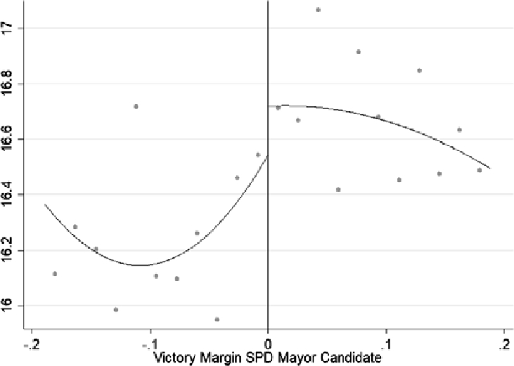
RD Plot: ln(Overall Exp.).
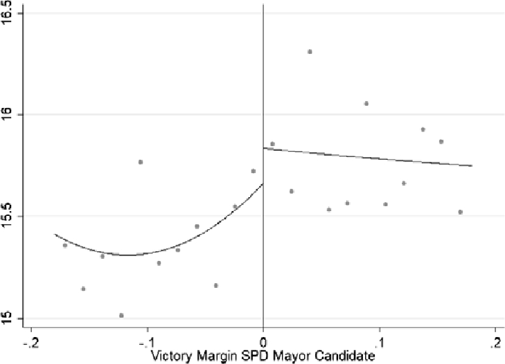
RD Plot ln(Financial Exp.).
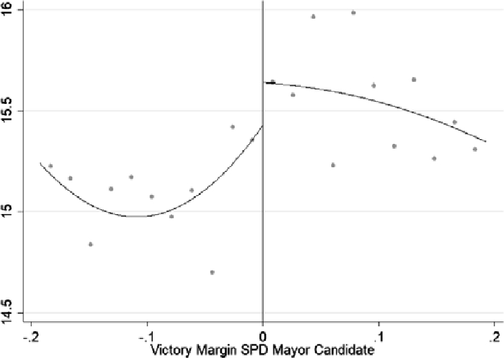
RD Plot: ln(Voluntary Exp.).
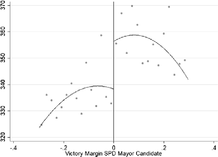
RD Plot: Business Tax Mult.
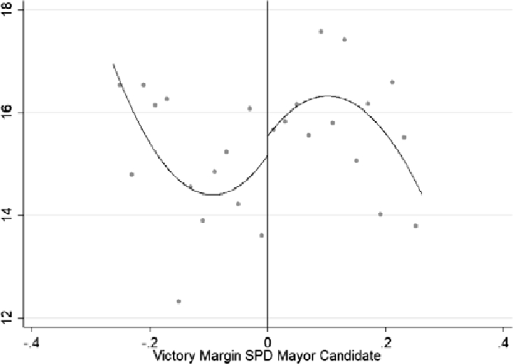
RD Plot: Share General Exp.
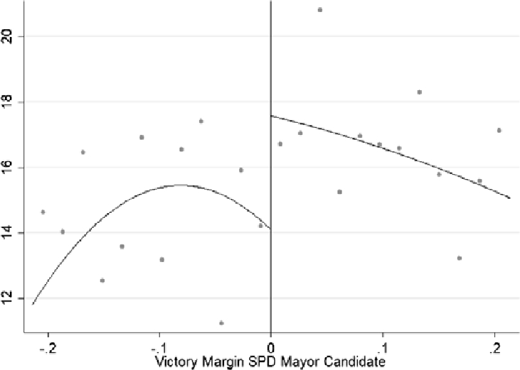
RD Plot: Share People Exp.
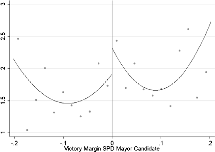
RD Plot: Share Culture Exp.
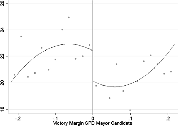
RD Plot: Share Infra. Exp.
References
Albouy, David. 2013. “Partisan Representation in Congress and the Geographic Distribution of Federal Funds.” The Review of Economics and Statistics 95(1): 127–141. 10.3386/w15224Search in Google Scholar
Alesina, Alberto. 1988. “Credibility and Policy Convergence in a Two-Party System with Rational Voters.” American Economic Review 78(4): 796–806. Search in Google Scholar
Besley, Timothy, and Anne Case. 2003. “Political Institutions and Policy Choices: Evidence from the United States.” Journal of Economic Literature 41(1): 7–73. 10.1920/wp.ifs.2002.0213Search in Google Scholar
Caillaud, Bernard, and Jean Tirole. 2002. “Parties as Political Intermediaries.” The Quarterly Journal of Economics 117(4): 1453–1489. 10.1162/003355302320935070Search in Google Scholar
Calonico, Sebastian, Matias D. Cattaneo, and Max H. Farrell. 2018. “On the Effect of Bias Estimation on Coverage Accuracy in Nonparametric Inference.” Journal of the American Statistical Association 113(522): 767–779. 10.1080/01621459.2017.1285776Search in Google Scholar
Calonico, Sebastian, Matias D. Cattaneo, and Rocio Titiunik. 2014. “Robust Nonparametric Confidence Intervals for Regression-Discontinuity Design.” Econometrica 82(6): 2295–2326. 10.3982/ECTA11757Search in Google Scholar
Calvert, Randall. 1985. “Robustness of the Multidimensional Voting Model: Candidate Motivations, Uncertainty, and Convergence.” American Journal of Political Science 29(1): 69–95. 10.2307/2111212Search in Google Scholar
Cattaneo, Matias D., Brigham R. Frandsen, and Rocío Titiunik. 2014. “Randomization Inference in the Regression Discontinuity Design: An Application to Party Advantages in the U.S. Senate.” Journal of Causal Inference 3:1–24. 10.1515/jci-2013-0010Search in Google Scholar
Cattaneo, Matias D., Michael Jansson, and Xinwei Ma. 2019. “Simple Local Polynomial Density Estimators.” Journal of the American Statistical Association. (forthcoming). 10.1080/01621459.2019.1635480Search in Google Scholar
Caughey, Devin, and Jasjeet S. Sekhon. 2011. “Elections and the Regression Discontinuity Design: Lessons from Close U.S. House Races, 1942–2008.” Political Analysis 19:385–408. 10.1093/pan/mpr032Search in Google Scholar
Cox, Gary W., and Mathew D. McCubbins. 1986. “Electoral Politics as a Redistributive Game.” The Journal of Politics 48(2): 370–389. 10.2307/2131098Search in Google Scholar
Curto-Grau, Marta, Albert Solle-Olle, and Pilar Sorribas-Navarro. 2018. “Does Electoral Competition Curb Party Favoritism?” American Economic Journal: Applied Economics 10(4): 378–407. 10.1257/app.20160618Search in Google Scholar
Downs, Anthony. 1957. An Economic Theory of Democracy. Boston, MA: Addison-Wesley. Search in Google Scholar
Eggers, Andrew, Anthony Fowler, Jens Hainmueller, Andrew Hall, and James Snyder. 2015. “On the Validity of the Regression Discontinuity Design for Estimating Electoral Effects: Evidence from over 40,000 Close Races.” American Journal of Political Science 59(1): 259–274. 10.1111/ajps.12127Search in Google Scholar
Ferreira, Fernando, and Joseph Gyourko. 2009. “Do Political Parties Matter? Evidence from U.S. Cities.” The Quarterly Journal of Economics 124(1): 399–422. 10.3386/w13535Search in Google Scholar
Fiva, Jon H., and Helene Lie Rohr. 2018. “Climbing the Ranks: Incumbency Effects in Party-list Systems.” European Economic Review 101:142–156. 10.1016/j.euroecorev.2017.09.011Search in Google Scholar
Fiva, Jon, Olle Folke, and Rune J. Sorensen. 2018. “The Power of Parties: Evidence from Close Municipal Elections in Norway.” The Scandinavian Journal of Economics 120(1): 3–30. 10.1111/sjoe.12229Search in Google Scholar
Folke, Olle. 2014. “Shades of Brown and Green: Party Effects in Proportional Election Systems.” Journal of the European Economic Association 12(5): 1361–1395. 10.1111/jeea.12103Search in Google Scholar
Freier, Ronny, and Christian Odendahl. 2015. “Do Parties Matter? Estimating the Effect of Political Power in Multi-Party Systems.” European Economic Review 80:310–328. 10.1016/j.euroecorev.2015.09.011Search in Google Scholar
Gerber, Elisabeth R., and Daniel J. Hopkins. 2011. “When Mayors Matter: Estimating the Impact of Mayoral Pininship on City Policy.” American Journal of Political Science 55(2): 326–339. 10.2139/ssrn.1475237Search in Google Scholar
Glaeser, Edward L., Giacomo A. M. Ponzetto, and Jesse M. Shapiro. 2005. “Strategic Extremism: Why Republicans and Democrats Divide on Religious Values.” The Quarterly Journal of Economics 120(4): 1283–1330. 10.3386/w10835Search in Google Scholar
Hainmueller, Jens. 2012. “Entropy Balancing for Causal Effects: A Multivariate Reweighting Method to Produce Balanced Samples in Observational Studies.” Political Analysis 20(1): 25–46. 10.1093/pan/mpr025Search in Google Scholar
Hotelling, Harold. 1929. “Stability in Competition.” Economic Journal 39:41–57. 10.1007/978-1-4613-8905-7_4Search in Google Scholar
Hyytinen, Ari, Jaakko Meriläinen, Tuukka Saarimaa, Otto Toivanen, and Janne Tukiainen. 2018. “When Does Regression Discontinuity Design Work? Evidence from Random Election Outcomes.” Quantitative Economics 9(2): 1019–1051. 10.3982/QE864Search in Google Scholar
Imbens, Guido W. 2004. “Nonparametric Estimation of Average Treatment Effects Under Exogeneity: A Review.” The Review of Economics and Statistics 86(1): 4–29. 10.3386/t0294Search in Google Scholar
Infratest-dimap. 2019. “Parteienkompetenz Europawahl 2019, Cited by Tagesschau 27.5.2019.” https://wahl.tagesschau.de/wahlen/2019-05-26-EP-DE/charts/umfrage-kompetenz/chart_379033.shtml (last accessed: June 2020). Search in Google Scholar
Kotakorpi, Kaisa, Panu Poutvaara, and Marko Terviö. 2017. “Returns to Office in National and Local Politics: A Bootstrap Method and Evidence from Finland.” The Journal of Law, Economics, and Organization 33(3): 413–442. 10.1093/jleo/ewx010Search in Google Scholar
Lee, David S. 2008. “Randomized Experiments from Non-random Selection in U.S. House Elections.” Journal of Econometrics 142(2): 675–697. 10.1016/j.jeconom.2007.05.004Search in Google Scholar
Lee, David S., Enrico Moretti, and Matthew J. Butler. 2004. “Do Voters Affect or Elect Policies? Evidence from the U.S. House.” The Quarterly Journal of Economics 119(3): 807–859. 10.1162/0033553041502153Search in Google Scholar
Levy, Gilat. 2004. “A Model of Political Parties.” Journal of Economic Theory 115(2): 250–277. 10.1016/S0022-0531(03)00254-0Search in Google Scholar
McCrary, Justin. 2008. “Manipulation of the Running Variable in the Regression Discontinuity Design: A Density Test.” Journal of Econometrics 142(2): 698–714. 10.3386/t0334Search in Google Scholar
Meriläinen, Jaakko. 2019. “Single Party Rule, Public Spending, and Political Rents: Evidence from Finnish Municipalities.” The Scandinavian Journal of Economics 121(2): 736–762. 10.1111/sjoe.12288Search in Google Scholar
Pappi, Franz Urban, and Gabriele Eckstein. 1998. “Voters’ Party Preferences in Multiparty Systems and Their Coalitional and Spatial Implications: Germany After Unification.” Public Choice 97(3): 229–255. 10.1007/978-1-4757-5127-7_2Search in Google Scholar
Persson, Torsten, Gerard Roland, and Guido Tabellini. 2007. “Electoral Rules and Government Spending in Parliamentary Democracies.” Quarterly Journal of Political Science 2(2): 155–188. 10.1561/100.00006019Search in Google Scholar
Pettersson-Lidbom, Per. 2008. “Do Parties Matter for Economic Outcomes? A Regression-Discontinuity Approach.” Journal of the European Economic Association 6(5): 1037–1056. 10.1162/JEEA.2008.6.5.1037Search in Google Scholar
Potrafke, Niklas. 2011a. “Does Government Ideology Influence Budget Composition? Empirical Evidence from OECD Countries.” Economics of Governance 12(2): 101–134. 10.1007/s10101-010-0092-9Search in Google Scholar
Potrafke, Niklas. 2011b. “Public Expenditures on Education and Cultural Affairs in the West German States: Does Government Ideology Influence the Budget Composition?” German Economic Review 12(1): 124–145. 10.1111/j.1468-0475.2010.00507.xSearch in Google Scholar
Snyder, James M., and Michael M. Ting. 2002. “An Informational Rationale for Political Parties.” American Journal of Political Science 46(1): 90–110. 10.2307/3088416Search in Google Scholar
Sole-Olle, Albert, and Elisabet Viladecans-Marsal. 2013. “Do Political Parties Matter for Local Land Use Policies?” Journal of Urban Economics 78:42–56. 10.1016/j.jue.2013.07.003Search in Google Scholar
Wittman, Donald. 1983. “Candidate Motivation: A Synthesis of Alternative Theories.” The American Political Science Review 77(1): 142–157. 10.2307/1956016Search in Google Scholar
© 2021 Walter de Gruyter GmbH, Berlin/Boston
Articles in the same Issue
- Frontmatter
- Original Articles
- Skimming through search
- Do political parties matter? Evidence from German municipalities
- In-group, out-group effects in distributional preferences: the case of gender
- Patents versus rewards: the implications of production inefficiency
- Income-(in)dependent equivalence scales and inequality measurement