With Whom Do Nations Trade? – The Fading Distance
-
Michael Michaely
 and
David Wajnryt
and
David Wajnryt

Abstract
Distance has conventionally been considered a major determinant of the direction of international trade. This contrasts, intuitively, with the generally-acknowledged fact that transportation costs are only a minor component of prices in international trade. The present study estimates the impact of distance on mutual trade flows in alternative, more direct methods than those employed traditionally in the literature. In particular, it looks at the “intensity ratio” in mutual trade; and asks to what extent its deviation from the size expected under an assumption of “neutrality” may be explained by mutual distances. It is found that, by and large, distance is a minor determinant of the trade of nations with each other. It is of some significance when trade flows within quite short ranges are concerned; but beyond these, the impact of distance on trade largely fades away.
1 The Issue [1]
The impact of distance on the size of trade among potential partners has been an important subject of the research of international trade flows in the last few decades. Appreciation of this impact is an essential component for issues such as the determination of promising partners for preferential trade agreements; or for consideration of the need for the grant of compensating special privileges in international agreements for countries with inherent weaknesses in the conduct of international trade. [2]
Most often, the study of the impact of distance has been conducted within the framework of the “gravity model” (or “gravity equation”). [3] Borrowing from the Newtonian equation in physics, this model starts with the presumption that the size of a trade flow between two partners is a function of “distance” and “mass” – geographic distance between the two representing the former, and the size of each partner’s income standing for “mass”. Within this framework, the impact of distance is separated and estimated.
Almost invariably, these “gravity-model” studies have found a predominant influence of distance on the size of trade flows. The elasticity of the trade–distance relationship appears most often to be in the range of unity and above [4]. Thus, for instance, doubling (hypothetically) the distance between two potential partners would cut their mutual trade flows by a half; and tripling the distance would lower the trade flows to just one third. This is a dramatic impact indeed. [5]
But these findings stand in obvious contradiction to estimates of the costs which must be involved in distance; especially transportation costs cannot possibly explain the presumed impact of distance on trade. Available studies of transportation costs come up with estimates in the range of 3–10 % of the cost excluding international transfer costs. That is, the C.I.F to F.O.B price ratio is in the range of 1.03–1.10. [6]
Moreover, marginal costs of (international) transportation must be substantially below average costs, since much of the transportation–costs components are of a fixed nature. This includes elements such as packing, loading and unloading of the cargo, waiting time in ports, or paper work such as consular registration, etc. Thus, for instance, doubling the distance a cargo has to travel should raise transportation costs by significantly less.
But even putting aside this difference between marginal and average, the change in transportation costs due to a change in distance must be rather trivial. Take, again, a doubling of distance, and suppose that transportation costs are 10 % of the F.O.B. price to start with, and that they double with the doubling of distance. The C.I.F. price would then increase by (almost) 10 % – from 1.1 to 1.2 of the F.O.B. price. Expecting such price change to lower the quantity demanded (and transacted) by a half would require an incredibly high elasticity of demand by the customer country – to levels which intuitively exceed any reasonable expectations.
This contradiction has certainly not escaped attention. In a general way, reconciliation has been attempted by observing that distance may not just imply a price differential, due to transportation costs, but may stand for other elements which should affect the size of mutual trade. One is a shared border: proximate countries may have common borders, which presumably tend to increase trade flows among partners. Other elements work in a similar way: proximate countries – more than others – may be expected to share important cultural attributes (a common language is obviously the most important), or to share histories, religion, legal or political systems – all of which are elements conducive to trade. But, while true, it should be noticed that the estimates of trade–distance elasticity mentioned earlier do, mostly, take these non-price elements into account; and try to separate them out (normally through the use of dummy variables). The afore-mentioned elasticities are thus derived after the impact of the non-price proximity elements has been abstracted from.
A more recent response to the apparent counter–intuitive estimates of the trade-distance elasticity is that “distance” stands primarily for “information costs”. This concept – which presumably incorporates other elements than those of the (estimated) impact of shared borders, shared language, etc. – is rather elusive and probably unquantifiable (except, as in the present argument, as an inference derived from residuals). To the extent that there is much substance to it, this might have been more relevant to earlier generations: at present, information salient to the conduct of transactions presumably flows freely and immediately over the globe. But even if this element were important, it would at most imply that proximate countries would better share information than others; it would definitely not imply that an “information barrier” somehow increases, with distance, beyond a certain threshold. That is, it would not yield a linear estimate of the impact of distance. It would rather call for a different method of estimation – perhaps through classification of countries into categories of “proximate” neighbors and others. Some such distinction will indeed be attempted in the present study.
We thus reach the almost inevitable conclusion that the impact of distance on trade inferred through the “gravity equation” estimates must have been grossly over-estimated. Perhaps a different approach may better serve for this task. To this we now turn.
2 Coverage and Construction of Observations
Our aim is to observe, in principle, all bilateral flows in today’s world trade; in practice we fall slightly short of it – but the discrepancy is insignificant.
Our basis of observations are trade data detailed by SITC for 2008. These are drawn from the United Nations commodity trade statistics database (COMTRADE).
We include in the study as many countries as would seem to be of some benefit without involving excessive costs. Trade data are available for the overwhelming majority of present independent (at least in the recording sense) countries and territories. These number (in 2008) 201. But inclusion of all of them would be cumbersome, costly, and partly not helpful: over half of these units are very minor actors, knowledge of which would add only little in the present context. [7] We have thus decided to cover in the study only countries whose trade amounts (individually) to at least one seventh of 1 % of world trade according to aggregated trade data published by the World Trade Organization. This leads to the inclusion of eighty two countries, whose combined trade amounted to 98.24 % of the world’s aggregate. From these, only countries for which detailed trade data are available at the COMTRADE database were included in the analysis. This leads to the inclusion of seventy countries, whose combined trade amounted to 92.24 % of the world’s aggregate. This surely enables the establishment of a solid foundation for an empirical analysis: the aggregate number of (potential) bilateral trade flows among these countries is as high as 4,761. The list of countries, with their volumes of trade, is presented in the Appendix.
The first basic set of observations we establish is, thus, the volumes of bilateral trade flows among countries. The second basic set is that of bilateral distances among all countries covered in the study. This is drawn from a file containing the great circle distance between capital cities (Gleditsch, Kristian. Capdist.csv. http://privatewww.essex.ac.uk/~ksg/data-5.html).
As we proceed, several other sets of data will be required; but these will be presented when the analyses for which they are used is discussed, further along in the study. [8]
We shall employ two alternative – though inevitably related – forms of analysis. These two will be used to either re-enforce or cast in doubt the inferences of each other. The next section will address one of these methods, which may be characterized as semi-impressionistic; whereas the other – more rigorous – will be discussed in the following section.
3 Distance and the Volume of Trade Flows
The method of analysis used in this section is rudimentary. Having two sets of variables, one of the volumes of bilateral trade flows and the other of distances, what is the relationship between the two?
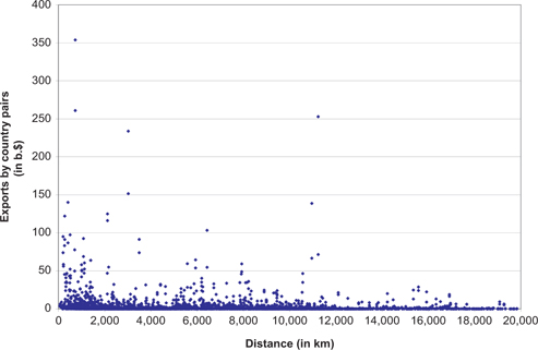
A rough impression may be gained, first, from a scatter diagram of the two variables – presented in Figure 1. The indication suggested by this diagram is of the existence of only little order; that is, of a weak relationship of the two variables to each other. To the extent that such relationship does exist, it appears to be found in the range of small distances. When this range is ignored, no order at all seems to prevail. Table 1 serves to pursue this line of investigation.
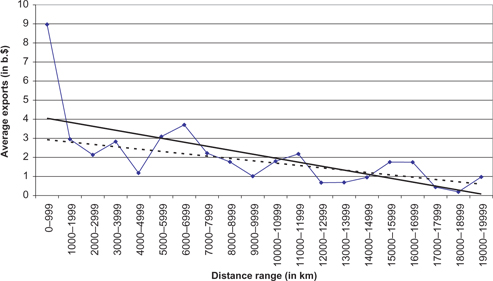
For ease of presentation and of drawing inferences, the universe of 4,629 observations is classified into 20 ranges of distances of 1,000 km each – from the first of 0 – 999 km to the last of 19,000 – 19,999 km. The number of observations in each distance range is recorded in column (2); the aggregate size of trade in each distance-range in column (3); and the average size of each trade flow within the range – in column (4). The relationship of the latter (average flow) to distance (range) is also presented by means of Figure 2.
Several inferences suggest themselves. First, a (negative) relationship of the size of a trade flow between partners to their distance from each other does exist. This is less than a surprise. But two important qualifications of this rule stand out. First, while a trend (of the relationship) does exist, fluctuations around the trend line are major. [9] Thus, the relationship is highly irregular. More important: the relationship is weak, in comparison with expectations of the conventional wisdom. For instance, sizes of the average trade flows read from the solid trend line in Figure 2 tell us that moving from a distance of 1,000–1,999 km (a mid-point of 1,500 km) to the distance of 7,000–7,999 km (a mid-point 7,500 km) – that is, multiplying distance by five-fold – would lower the trade flow by just 35 %, whereas a unit elasticity of trade to distance would predict the reduction of trade by as much as 80 %.
Second, an inference which clearly suggests itself is the overwhelming impact of trade within the shortest distance range on any overall trend of the trade–distance relationship. Within the first range category, that of 0–999 km, some 27 % of aggregate world trade is conducted, and the size of the average trade flow within this distance range is far higher than at any other range. The impact of trade flows within this shortest range must thus be of major importance for general rules which are found to characterize the relationship of trade to distance. The exclusion of transactions conducted within just this range must, hence, weaken – probably crucially so – the apparent relationship of trade to distance. In Figure 2 the dashed line represents the trend line of this relationship, when the first distance category (0–999 km) is excluded from the universe of observations. This appears to be a substantially flatter line – representing, that is, a weaker relationship between distance and the volume of trade.
We add to these findings by estimating the trade–distance relationship in the universe of observations (rather than by classification into distance ranges). This relationship is estimated by the simple regression.
where j, k are two trade partners;
Distance range and trade flows.
| Distance range (in km) (1) | No. of observations (2) | Aggregate exports (in b.$) (3) | Average exports (in b.$) ((3)/(2)) (4) | ||
| 1 | 0 | 999 | 369 | 3,309 | 8.96 |
| 2 | 1,000 | 1,999 | 670 | 1,977 | 2.95 |
| 3 | 2,000 | 2,999 | 430 | 916 | 2.13 |
| 4 | 3,000 | 3,999 | 349 | 986 | 2.82 |
| 5 | 4,000 | 4,999 | 310 | 366 | 1.18 |
| 6 | 5,000 | 5,000 | 260 | 803 | 3.09 |
| 7 | 6,000 | 6,999 | 201 | 745 | 3.70 |
| 8 | 7,000 | 7,999 | 226 | 501 | 2.22 |
| 9 | 8,000 | 8,999 | 303 | 533 | 1.75 |
| 10 | 9,000 | 9,999 | 374 | 376 | 1.00 |
| 11 | 10,000 | 10,999 | 290 | 521 | 1.80 |
| 12 | 11,000 | 11,999 | 223 | 486 | 2.18 |
| 13 | 12,000 | 11,999 | 120 | 80 | 0.67 |
| 14 | 13,000 | 13,999 | 95 | 65 | 0.68 |
| 15 | 14,000 | 14,999 | 83 | 79 | 0.55 |
| 16 | 15,000 | 15,999 | 84 | 147 | 1.75 |
| 17 | 16,000 | 16.999 | 77 | 134 | 1.74 |
| 18 | 17,000 | 17,999 | 66 | 29 | 0.44 |
| 19 | 18,000 | 18,999 | 48 | 9 | 0.19 |
| 20 | 19,000 | 19.000 | 31 | 30 | 0.97 |
| All observations | 4,629 | 12,095 | 2.61 | ||
| Excluding range (1) | 4,260 | 8,786 | 2.06 | ||
| Range (1) | 369 | 3,309 | 8.96 | ||
Distance and trade flows.
Distance range and trade flows.
The outcome is presented in Table 2. It is first seen, from line (1), that the relationship of the two variables is weak – the R2 of the equation is very low. The coefficient of the trade–distance relationship appears to be high – it is – 0.852; but just the exclusion of the lowest distance range (0 – 999 km) lowers the coefficient to –0.249 as well as lowering the R2 to practically zero.
The particularly strong (relatively speaking) relationship of trade to distance at the lowest range of the latter raises an important issue. Suppose countries in this distance range amongst them are not only close (by definition) to each other but also large in their trade volumes. A sizable trade between each such pair of countries may be expected regardless of distance – arising simply from the fact that the potential partner is a heavy trader. The estimated trade–distance relationship would thus yield a misleading inference. This is not just a hypothetical suggestion: very important segments of geographically–close nations are particularly large trading nations – primarily in Europe, but also in North-America.
The next section will employ a method of inquiry which would free the investigation from the impact of the size of the trading partner, thus revealing purely the relationship between distance and trade flows. [10] We now move to it.
4 Distance and Trade Intensity
The basic measure for the study of trade–distance relationship in the following is the well-known “intensity ratio”:
where, j, k are two trade partners (j is the home country);
A ratio of unity would tell us that the share of country j’s exports to partner k out of j’s aggregate exports is identical to the share of partner k in aggregate world imports; that is, that the size of this trade flow is “explained” by the weight of the partner in world imports. This would be, thus, an expression of “neutrality” in the trade relationship at hand – with no bias involved. A ratio below unity would represent a negative bias and a ratio above unity – a positive bias. [12] “Bias” has, in this context, no normative connotation: it is just the expression of the tendency of one country to trade with a partner differently from what the sheer size of the latter as a trader would call for. That is, it reflects the existence of factors other than the size (in trade) of a partner which participate in determining the size of a trade flow with a partner.
A variety of such factors would suggest themselves. The salient ones mostly are mentioned in “gravity-model” analyses. An obvious factor that comes to mind is distance – the element to which the present analysis is mostly addressed. The question we pose, thus, is: to what extent may the (positive or negative) “bias” in trade flows among partners be explained by distance among them?
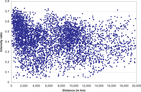
Space limitations do not allow the full presentation here of the matrix of export intensity ratios, nor for the matrix of bilateral distances. [13] Instead, Figure 3, similarly to Figure 1 earlier, presents a scatter diagram of the relationship of distance to the intensity ratio in trade.
The visual inference which appears from the chart is clear cut: (1) To the extent that there is any relationship of the intensity of trade to distance, it must be weak; and (2) That such relationship might perhaps be stronger for trade flows conducted within relatively short distances, than for longer distances (this obviously agrees with a similar inference suggested earlier). We now turn to the formal analysis of such hypotheses.
Table 3 presents the findings of a simple regression analysis in which the intensity ratio of a trade flow is explained by the distance between the two partners to the flow. To add some perspective, we also present in the table (row d) the outcome of a similar procedure applied to trade data of 1963. Naturally, the coverage of the latter is narrower than the 2008 data, due to a smaller number of independent nations and a less inclusive data coverage – only 43 countries are represented. But this is enough for the purpose at hand, particularly since almost all the substantial traders are included Several inferences emerge from the findings.
Relationship of trade flows to distance.
| No. of observation (1) | Adj R2 (2) | t value (3) | Distance coefficient (4) | |
| a. All observations | 4,609 | 0.073 | –19.11 | –0.852 |
| b. Distance above 2,500 km | 3,563 | 0.002 | –2.79 | –0.249 |
Dependent Variable=log value of exports; independent variable=log distance.
Relationship of trade intensity to distance.
| No. of observations (1) | Adj R2 (2) | t value (3) | Distance coefficient (4) | |
| a. All observations | 4,690 | 0.050 | –15.78 | –0.094 |
| b. Distance below 2,500 km. | 1,076 | 0.031 | –5.97 | –0.106 |
| c. Distance above 2,500 km | 3,614 | 0.000 | –0.81 | –0.009 |
| d. Data for 1963 | 1,722 | 0.069 | –11.30 | –0.117 |
Distance and trade intensity.
For the universe of observations, a rather weak relationship between the two variables is indicated: the R2 is about 0.050 – that is, quite low. The elasticity of the size of trade to changes in distance [14] appears to be roughly –0.09. This is radically different from the unit elasticities (or above) found by the recorded “gravity equation” analyses. To the extent that it is meaningful, this elasticity should be in conformity with the levels of transportation costs referred to earlier.
The relationship between the two variables improves somewhat when observations are confined to the range below 2,500 km. The R2 remains low, at 0.031; but the elasticity of trade to distance increases slightly to close to –0.11. For the range of distances above 2,500 km, on the other hand, the relationship between the two variables practically disappears. [15] This, again, would conform with the observation made earlier about the presumably low level of marginal (to distance) costs. The indications provided by Table 3 are, thus, not surprising.
The salient findings represent, most probably, fundamental, long-term structures of trade. The estimated coefficients for 1963 (row d) are very close to those of 2008 (row a). A thorough investigation of changes over time would obviously require more than the analysis presented here. Yet, it would seem unlikely that major fluctuations (of the relevant coefficients) took place, back and forth, during the decades between the early 1960s and the end of the first decade of the twenty-first century.
5 Distance Joined with Other Explanatory Variables
Apart from distance, several other factors may be expected to have an impact on the “bias” in the direction of trade flows. We shall now add them to the analysis.
The first two such attributes are well known and, as we have mentioned earlier, have been widely explored in the literature. These are:
Shared borders of the two partner countries to a trade flow. Not much need be said about this: both a–priori expectation and much research have pointed to its significance in expanding trade between potential partners.
Shared cultures, histories, and institutions. Once more, a–priori reasoning would certainly assign significance to these attributes in expanding bilateral trade flows. Empirical research is, in this case, less feasible, since these attributes cannot easily be quantified and measured. Mostly, they are represented by the existence of just one attribute, namely, a common language of the two partners.
These two variables are clearly related to distance, expected to be manifested the closer the two partners to each other. For shared borders, this holds almost by definition; [16] but the relationship must be strong also when cultural affinities (represented by a common language) are concerned. Hence, the explicit addition of these two variables to the analysis should serve to weaken the apparent relationship of trade intensities to distance. In fact, though, while pointing out the relevance of these attributes, their impact will not be shown in the following statistical analysis, for a simple reason: the analysis attempted with their inclusion showed no relationship of the two to trade intensities. This may be due to their small representation: among over 4,500 observations, those which encompass shared borders or common language amount only to a few hundreds, each.
We are thus left with two other variables, which are less commonly addressed and which deserve, hence, a few words of explanation. It should be observed that both these variables are not expected on a–priori grounds, to be related to distance.
Trade compatibility. Trade between two potential partners may be expected to be higher the more does one partner have to offer of what the other partner demands. This matching of desires and offers may be viewed through the compatibility of trade structures, namely: the more does one potential partner export goods which loom large in the other partner’s import structure, the more, ceteris paribus, should the two nations trade with each other. In the extreme (negative) case, when one partner exports none of the goods which the other imports, no trade between the two should be expected. On the other extreme, trade would be maximized when the export structure of one partner is identical with the other’s import structure. This relationship of the export–import structures of the two potential partners is represented by the index of compatibility of trade structures. The index is defined as follows: [17]
where, j, k are two trade partners; SXiMk= index of compatibility of exports of country j and imports of country k; ׀ ׀ indicates absolute values; Xij=share of good i in j’s exports; and Mik=share of good i in k’s imports.
Similarity of income levels. There are several reasons why similarity, or absence thereof, of income levels of two potential partners should be a factor which participates in determining the size of trade between them; but two basic considerations point in opposite directions. Per-capita income levels represent, by and large (with some notable exceptions) levels of development and indicators of structures of economies. Disparity of income levels should thus be related to dissimilarity of economic structures; and, in particular, of relative scarcity or abundance, and of relative prices, of factors of production – in particular, of natural resources and unskilled labor vs. capital and skilled labor. The larger this disparity, the larger should be the “Heckscher-Ohlin” type of trade between the partners. On the other hand, the more similar the two economies, the more should the demand patterns of the two be compatible, and, for by now well–known reasons, the stronger should be the intra–industry trade flows between the two. Due to this ambiguity, it is not certain, on a–priori grounds, whether similarity of income levels should be a positive or a negative factor in determining the size of trade flows between partners. But since it might be an important element, one way or another, its inclusion among the explanatory variables of trade intensity seems to be warranted.
The degree of dissimilarity between the income levels is defined simply as
The relationship between the intensity ratio in trade (exports) and the three explanatory variables (distance, compatibility, and dissimilarity of income levels) is formulated by:
where j, k are two trade partners (j is the home country);
Trade intensity and explanatory variables.
| Variable (1) | Parameter estimate (2) | t value (3) |
| a. Exports | ||
| No. of observation=4,609; Adj R2=0.167 | ||
| Intercept | –0.713 | –11.05 |
| Distance | –0.028 | –4.64 |
| Compatibility | 0.066 | 25.17 |
| Income differential | 0.012 | 2.91 |
| b. Imports | ||
| No. of observations=4,646; Adj R2=0.160 | ||
| Intercept | –0.065 | –10.15 |
| Distance | –0.037 | –6.18 |
| Compatibility | 0.069 | 24.14 |
| Income differential | 0.013 | 3.23 |
The estimation is applied to the log form of the variables. The coefficients λ, β,γ. thus constitute the elasticities of the trade flow to changes in the respective explanatory variables. The findings are presented in Table 4. Several salient inferences may be drawn from these findings:
First, despite the addition of other explanatory variables, all of these together offer only a minor explanation of the level of intensity ratios; the adjusted R2 appears to be only around 0.16.
Second, the elasticity of trade to distance appears to be – as might be expected – even lower than in the absence of other (than distance) explanatory variables; it appears now to be at the level of –0.03 to –0.04.
Third, the elasticity of trade to the level of compatibility of respective trade flows appears to be higher than that applying to distance – around 0.07 (the t values, as well, are much higher here). This implies that, in explaining the intensity of trade between two potential partners the structures of their (aggregate) trade flows should not be ignored.
Fourth, dissimilarities of income levels of two partners seem to have a positive impact on the intensity of their mutual trade. But it is weak. The interpretation of this finding when it is this low is not clear cut, since it presumably reflects, as has been discussed before, the net impact of contradictory (in sign) effects of the variable at hand on mutual trade.
6 Summary and Conclusions
The “conventional-wisdom” perception of the relationship between geographical distance and trade flows among potential partners, based on a large number of empirical findings drawn from gravity analyses, is that distance has a strong impact on trade: typically the elasticity estimates of trade to distance found in these studies run around unity. This stands in stark contrast to estimates of transportation costs, which imply that increasing distances should add only little to price. The present study examines directly the trade–distance relationship, to try to see whether the “conventional wisdom” may not be mistakenly held.
The study encompasses around seventy countries, with over 4,500 bilateral trade flows among them. It uses two alternative forms of analysis. One is the observation of the relationship between trade and distance yielded directly by data of trade flows. The other is based on “intensity ratios” of trade, and asks to what extent distance may explain the “bias” in mutual trade relationships – that is, the extent to which the size of a trade flow differs from what would be derived from a “neutral” assumption that the specific trade flow is just a function of aggregate trade volumes of the two potential partners.
Both methods yield similar inferences. These are:
First, a (negative) relationship between bilateral trade flows and bilateral distances does exist – it would be highly surprising if it were not. But this relationship appears to be weak – far from the strength expected from commonly–accepted estimates. This finding does agree with observations of transportation costs being, by and large, a quite minor component of prices in world trade.
Second, the relationship at hand tends to be somewhat stronger when relatively short distances are examined; and to almost vanish over long distances. This, once more, agrees with the presumption that marginal transportation costs are substantially lower than average costs; it would also be compatible with the assumption that “distance” represents factors other than measurable transportation costs, such as (vaguely defined) “information costs”, similarity among partners of legal systems, institutions, commercial rules, or cultural ties. All these potential elements would presumably exist between close neighbors; but they should not change much when gradually rising distances are concerned.
Third, among other (than distance) factors which might explain the strength (or weakness) of trade ties between potential partners the compatibility of export and import structures between any pair of countries – the degree to which one’s exports structure (hence export supply) is similar to the other’s import structure (hence import demand) – suggests itself as a significant element.
Intuition tells us that the size of trade flows between partners is influenced (negatively) by their distance from each other. This expectation is, not surprisingly, borne out by the findings of the present study: an impact of distance on trade does exist. Like the proverbial Old Soldiers, distance is not dead: it just fades away. The impact of distance appears to be weak – far weaker than prior studies would have led us to believe. By and large, distance does not appear to be a dominant factor in determining trade flows among nations. It largely loses relevance beyond a fairly short range.
It is always tempting – indeed, almost a methodological imperative – to try to explain phenomena and relationships in the context of a coherent model. The “gravity equation” does perform this task. But one of its principal findings – concerning the impact of distance – appears to be in doubt. The present study does not presume to suggest an alternative model. Its findings do imply, however, that the analysis of relationships of trade flows among nations requires additional components, which apparently outweigh by far the impact of distance. Some of these may probably best be assembled under the designation of “history”; that is, phenomena and attributes which must have been important in the past and whose impact persists today, though they may no longer exist now, nor may they feasibly be quantified and estimated.
Annex A: Trade Patterns of Small Countries
In discussions with colleagues, two issues which might have influenced our inferences have been raised. One is the possibility that by excluding from the study very small countries (in size of trade) we may have introduced a bias; that the impact of distance on trade patterns of small countries may be different from that prevalent in the larger ones. The other issue: our observations involve only positive trade flows; hence, they ignore the possibility that distance may have a consistent impact on the complete absence of trade among nations, and ignoring this potential may have biased our inferences.
The present Annex will be devoted to the first issue; namely, it will investigate the trade flows of very small countries; whereas the next – Annex B – will address the second, namely, the potential impact of distance on the complete absence of trade.
In a basic sense, the trade flows of very small countries are of minor consequences for the observation of world trade. The aggregate trade of countries excluded (due to size) from the main body of this study amounts, roughly, to just one tenth of aggregate world trade. Thus, this trade should have only minor implications for inferences regarding global trade patterns. But it may still be of some use to explore the possibility that trade patterns of very small countries (which we shall refer to as “ultra small”) differ, where the impact of distance is involved, from those of their large partners.
Off-hand, it does not appear on a-priori grounds that the relationship between trade flows and distance of partners should be consistently different – one way or another – in trade of small vs larger partners. Casual impressions of trade patterns do not suggest such bias either. But we shall not be content with such observations; and shall pursue here a more rigorous analysis.
This will be done by following a similar procedure to the one practiced in the main body of the study. First, we identify 71 “ultra small” countries. [18] In principle, we include here all world countries – 107 altogether – which are not covered in the main study. But, as might be expected, the required data (that is, data for both trade flows and distance) are often missing. These 71 “ultra small” countries will be our group of reference. [19] For convenience, we shall refer to the countries included in the main study as “large” – though they range from some that are very large indeed (the U.S., Germany) to many which are pretty small (in terms of their shares in world trade). The intensity ratios of trade between each ultra-small and each large country (once more, for exports) will be estimated; and then, related to distance between each pair of countries.
Altogether, close to 3,500 observations are recorded (3,489 to be precise). This is a sufficiently large number for drawing solid inferences – certainly of the nature we look for here; and the outcome of the analysis is indeed clear cut. A regression analysis (of the export intensity ratio over distance) yields the following coefficients:
Ad1 R2 = 0.020
Regression coefficient=–0.001
t value=–8.47
The outcome is obviously highly significant; and it shows practically no relationship between the intensity of trade and the distances among trading partners. This is even a much stronger finding than that of the main study in which such relationship, though pretty weak, does exist. The salient inference, for our purpose, is that the estimated impact of distance on trade indicated in the main body of the study could not be biased downwards by the exclusion from the study of “ultra small” countries. If anything, this exclusion must have led to an upward bias of the impact of distance on trade patterns.
Annex B: Distance and the Absence of trade
An exploration of the potential impact of distance on the complete absence of trade among potential partners requires some deviation from the conventional estimation of elasticities. If a change in one (the explanatory) variable leads to the reduction of the other (the explained one) to zero, the presumed elasticity is infinite. But this is not of much relevance: all elasticities in such cases would be infinite – regardless of the extent of the impact of one variable on the other. And, of no less importance, the inclusion of any such individual case within a “basket” or a group, would make the elasticity of the relationship at hand infinite for the whole group, regardless of the weight of the item concerned in the group (as long as it is positive). Hence, some alternative method of estimating the potential impact of distance on the absence of trade must be devised. We suggest here one such approximation.
Similar to the procedure in the main study, we construct a matrix of bilateral trade flows among each pair of countries. But instead of recording the size of trade (the “intensity ratio”), we use a binary classification: a “zero” if trade in this “box” is completely absent; and “one” when some trade does take place. Alongside with this, we record the distance between the countries involved. In each box of the matrix two magnitudes are thus recorded: “zero” or “one”, and distance. The assembly of all observations in all the boxes will then provide a series of the association of the two variables: distance and absence (or existence) of trade. A regression of the “zero-one” recorded observation on the recorded distance should thus yield an elasticity of the relationship of the two – different from the conventional one but an “elasticity” nevertheless.
Altogether, over 4,500 “boxes”, or units of observation, are constructed. A presentation of the full matrix would obviously not be feasible here. Instead, we present a summary table in which all observations are classified (in the same manner as in Table 1) into groups of distance, 1,000 km, each (0–999; 1,000–1,999; etc.). These groups are presented in Column (1) of Table 5, Column (2) of the table records, for information, the number of observations (“boxes”) in each distance category; whereas Column (3) presents the (unweighted) mean of the frequency of “zero” trade in each distance category.
The impression gained from this presentation is of the existence of a large variance among the groups; but no consistent relationship of frequency of “zero’s” to distance is apparent. Based thus on such impression, no clear impact of geographic distance on the existence or absence of trade flows among potential partners is indicated.
Frequency of absence of trade (“zero’s”), by distance.
| Distance range (km) | Number of observations | Frequency (in %) |
| 0–999 | 348 | 23.4 |
| 1,000–1,999 | 634 | 24.5 |
| 2,000–2,999 | 428 | 17.5 |
| 3,000–3,999 | 358 | 12.5 |
| 4,000–4,999 | 310 | 8.5 |
| 5,000–5,999 | 262 | 7.5 |
| 6,000–6,999 | 204 | 6.1 |
| 7,000–7,999 | 224 | 6.7 |
| 8,000–8,999 | 304 | 8.9 |
| 9,000–9,999 | 372 | 13.7 |
| 10,000–10,999 | 284 | 12.6 |
| 11,000–11,999 | 220 | 11.2 |
| 12,000–12,999 | 120 | 6.5 |
| 13,000–13,999 | 98 | 5.9 |
| 14,000–14,999 | 86 | 7.3 |
| 15,000–15,999 | 82 | 9.4 |
| 16,000–16,999 | 78 | 9.9 |
| 17,000–17,999 | 64 | 11.1 |
| 18,000–18,999 | 48 | 16.1 |
| 19,000 and upwards | 32 | 22.5 |
| 4,556 |
We now move to a more rigorous analysis.
A regression analysis of the two variables (dependent; frequency of “zero’s”; independent-distance), involving all (over 4,500) observations, yields the following
Ad1 R2 = 0.010
Regression coefficient=0.073
t value=–20.42
| Country | Share | Cumulative | Country | Share | Cumulative |
| 1. Germany | 8.97 | 8.97 | 42. Algeria | 0.49 | 89.25 |
| 2. China | 8.88 | 17.85 | 43. Kazakhstan | 0.44 | 89.69 |
| 3. U.S | 7.99 | 25.84 | 44. Slovak Rep. | 0.44 | 90.13 |
| 4. Japan | 4.85 | 30.69 | 45. Argentina | 0.43 | 90.56 |
| 5. Netherlands | 3.96 | 34.65 | 46. Ukraine | 0.42 | 90.98 |
| 6. France | 3.82 | 38.47 | 47. Chile | 0.41 | 91.39 |
| 7. Italy | 3.37 | 41.84 | 48. Angola* | 0.40 | 91.79 |
| 8. Belgium | 2.93 | 44.77 | 49. Libya* | 0.39 | 92.18 |
| 9. Russia | 2.93 | 47.69 | 50. Vietnam | 0.39 | 92.57 |
| 10. U.K | 2.85 | 50.55 | 51. Iraq* | 0.39 | 92.95 |
| 11. Canada | 2.83 | 53.38 | 52. Israel | 0.38 | 93.34 |
| 12. Korea, Rep. of | 2.62 | 56.00 | 53. Qatar | 0.35 | 93.69 |
| 13. Hong Kong (China) | 2.30 | 58.29 | 54. Portugal | 0.35 | 94.03 |
| 14. Singapore | 2.10 | 60.39 | 55. Romania | 0.31 | 94.34 |
| 15. Saudi Arabia* | 1.94 | 62.34 | 56. Philippines | 0.30 | 94.64 |
| 16. Mexico | 1.81 | 64.15 | 57. Oman | 0.23 | 94.88 |
| 17. Spain | 1.75 | 65.89 | 58. Colombia | 0.23 | 95.11 |
| 18. Taipei (Chinese)* | 1.59 | 67.48 | 59. Slovenia | 0.21 | 95.33 |
| 19. U. Arab Emirate | 1.48 | 68.96 | 60. Belarus | 0.20 | 95.53 |
| 20. Switzerland | 1.24 | 70.20 | 61. Peru | 0.20 | 95.72 |
| 21. Malaysia | 1.24 | 71.44 | 62. Azerbaijan | 0.19 | 95.91 |
| 22. Brazil | 1.23 | 72.67 | 63. New Zealand | 0.19 | 96.10 |
| 23. India | 1.21 | 73.88 | 64. Egypt | 0.16 | 96.26 |
| 24. Australia | 1.16 | 75.04 | 65. Greece | 0.16 | 96.42 |
| 25. Sweden | 1.14 | 76.18 | 66. Luxemburg | 0.16 | 96.58 |
| 26. Austria | 1.13 | 77.30 | 67. Lithuania | 0.15 | 96.73 |
| 27. Thailand | 1.10 | 78.41 | 68. Bulgaria | 0.14 | 96.87 |
| 28. Norway | 1.07 | 79.48 | 69. Pakistan | 0.13 | 96.99 |
| 29. Poland | 1.06 | 80.54 | 70. Morocco | 0.13 | 97.12 |
| 30. Czech Rep. | 0.91 | 81.45 | 71. Tunisia | 0.12 | 97.24 |
| 31. Indonesia | 0.87 | 82.31 | 72. Trinidad & Tob* | 0.12 | 97.36 |
| 32. Turkey | 0.82 | 83.13 | 73. Ecuador | 0.11 | 97.47 |
| 33. Ireland | 0.78 | 83.91 | 74. Bahrain* | 0.11 | 97.58 |
| 34. Denmark | 0.72 | 84.64 | 75. Equat. Guinea* | 0.10 | 97.68 |
| 35. Iran, Islamic Rep.* | 0.71 | 85.34 | 76. Bangladesh* | 0.10 | 97.78 |
| 36. Hungary | 0.67 | 86.01 | 77. Syria | 0.09 | 97.86 |
| 37. Finland | 0.60 | 86.61 | 78. Croatia | 0.09 | 97.95 |
| 38. Venezuela | 0.59 | 87.20 | 79. Estonia | 0.08 | 98.03 |
| 39. Kuwait | 0.54 | 87.74 | 80. Turkmenistan* | 0.08 | 98.10 |
| 40. Nigeria | 0.51 | 88.25 | 81. Sudan* | 0.07 | 98.17 |
| 41. South Africa | 0.50 | 88.75 | 82. Serbia | 0.07 | 98.24 |
The estimated “elasticity” of this dependence is thus close to zero. In addition, as the size of the coefficient of variance indicated, distance plays practically no role in explaining the frequency of “zero’s”. A strong conclusion thus emerges: Complete absence of trade among potential partners is not a function of distances among partners.
Appendix: Shares in World Exports – 2008
(In percent of world exports: in descending order)
(Total world exports=16,117 b.$)
References
Anderson, J. E. 1979. “A Theoretical Foundation for the Gravity Equation.” American Economic Review 69:106–116.Search in Google Scholar
Bergstrand, J. H. 1985. “Gravity Equation in International Trade: Some Micro-economic Foundations and Empirical Evidence.” Review of Economics and Statistics 67:474–481.10.2307/1925976Search in Google Scholar
Bergstrand, J. H. 1990. “The Heckscher-Ohlin-Samualson Model, the Lynder Hypothesis and the Determinants of Bilateral Intra-industry Trade.” Economic Journal 100:1216–1229.10.2307/2233969Search in Google Scholar
Disdier, Anne-Célia and Keith Head, “The Puzzling Persistence of the Distance Effect on Bilateral Trade”, Review of Economics and Statistics, 90:37–48.10.1162/rest.90.1.37Search in Google Scholar
Grynberg, R. (Ed.). 2006. WTO at the Margins: Small States and the Multilateral Trading System. Cambridge: Cambridge University Press.10.1017/CBO9780511674495Search in Google Scholar
Helpman, E., M. Melitz, and Y. Rubinstein. 2008. “Estimating Trade Flows, Trading Partners and Trading Volumes.” Quarterly Journal of Economics 123:441–448.10.3386/w12927Search in Google Scholar
Hummels, D. 2001. “Towards a Geography of Trade Costs”, unpublished manuscript, Purdue University.10.2139/ssrn.160533Search in Google Scholar
Linneman, H. 1966. An Econometric Study of International Trade Flows. Amsterdam: North-Holland Publishing Co.Search in Google Scholar
Michaely, M. 2009. Trade Liberalization and Trade Preferences (Revised Edition). Singapore: World Scientific Publishing Co.10.1142/6918Search in Google Scholar
Moneta, C. 1959. “The Estimation of Transportation Costs in International Trade.” Journal of Political Economy 67:41–58.10.1086/258129Search in Google Scholar
Redding, S., and A. J. Venables. 2006. “The Economics of Isolation and Distance.” Ch. 5 in WTO at the Margins, op-cit.10.1017/CBO9780511674495.006Search in Google Scholar
Tinbergen, J. 1962. Shaping the World Economy: Suggestions for an International Economic Policy. New York: The Twentieth Century Fund.Search in Google Scholar
©2016 by De Gruyter
Articles in the same Issue
- Frontmatter
- Articles
- With Whom Do Nations Trade? – The Fading Distance
- Long-Run Economic Growth: Stagnations, Explosions and the Middle Income Trap
- Self-Fulfilling and Fundamentals Based Speculative Attacks: A Theoretical Interpretation of the Euro Area Crisis
- Is India Ready for Inflation Targeting?
- Inward and Outward Foreign Direct Investment and Inequality: Evidence from a Group of Middle-Income Countries
- India-Us Trade and Investment: Have They Been Up To Potential?
- How do Liberalization, Institutions and Human Capital Development affect the Nexus between Domestic Private Investment and Foreign Direct Investment? Evidence from Sub-Saharan Africa