A compartmental model of the COVID-19 pandemic course in Germany

Yıldırım Adalıoğlu; Çağan Kaplan

doi:10.1515/em-2022-0126

Article Publicly Available

A compartmental model of the COVID-19 pandemic course in Germany

Yıldırım Adalıoğlu and Çağan Kaplan

Published/Copyright: June 29, 2023

Published by

Become an author with De Gruyter Brill

Submit Manuscript Author Information

From the journal Epidemiologic Methods Volume 12 Issue 1

Abstract

Objectives

In late 2019, the novel coronavirus, known as COVID-19, emerged in Wuhan, China, and rapidly spread worldwide, including in Germany. To mitigate the pandemic’s impact, various strategies, including vaccination and non-pharmaceutical interventions, have been implemented. However, the emergence of new, highly infectious SARS-CoV-2 strains has become the primary driving force behind the disease’s spread. Mathematical models, such as deterministic compartmental models, are essential for estimating contagion rates in different scenarios and predicting the pandemic’s behavior.

Methods

In this study, we present a novel model that incorporates vaccination dynamics, the three most prevalent virus strains (wild-type, alpha, and delta), infected individuals’ detection status, and pre-symptomatic transmission to represent the pandemic’s course in Germany from March 2, 2020, to August 17, 2021.

Results

By analyzing the behavior of the German population over 534 days and 25 time intervals, we estimated various parameters, including transmission, recovery, mortality, and detection. Furthermore, we conducted an alternative analysis of vaccination scenarios under the same interval conditions, emphasizing the importance of vaccination administration and awareness.

Conclusions

Our 534-day analysis provides policymakers with a range of circumstances and parameters that can be used to simulate future scenarios. The proposed model can also be used to make predictions and inform policy decisions related to pandemic control in Germany and beyond.

Keywords: compartmental models; computational epidemiology; COVID-19; extended SEIR models; Germany

Introduction

SARS-CoV-2, a new mutant from the Coronaviridae family was first detected in Wuhan, China in 2019 (Velavan and Meyer 2020; Wu and McGoogan 2020). After the detection of the virus, there has been a huge impact on many countries. Shortly, COVID-19 became a pandemic, spreading around the globe. To understand this infectious disease’s contagion better, one can use mathematical tools to model it. There have been numerous studies that build upon classical models. Several contemporary models have been developed to analyze the pandemic course in different countries. Examples include the SIDARTHE model developed by Giordano et al. for Italy (Giordano et al. 2020), a compartmental model developed by Barbarossa et al. for the COVID-19 pandemic in Germany (Barbarossa et al. 2020), and an extended SEIR model with vaccination for COVID-19 in Saudi Arabia (Ghostine et al. 2021). In this paper we have developed a novel model that encompasses compartments that are Susceptible, Vaccinated, Exposed, Detected Infected, Undetected Infected, Detected Recovered, Undetected Recovered, and Deceased. Additionally, Exposed, Detected Infected, and Undetected Infected compartments are divided into three main sub-compartments, according to the three most common strains of SARS-CoV-2 in Germany; which are the wild-type, alpha, and delta. We assumed the population remained constant; so births and natural deaths outside of COVID-19 were not taken into account.

One of the main purposes of this mathematical model is especially to predict the population dynamics of the Undetected Infected compartment whose data cannot be obtained by regulation. Even though this compartment has no practically obtainable data, it is a crucial compartment that contributes to contagion, therefore the continuum of the COVID-19 pandemic.

Additionally, it is critical to analyze the effects of the COVID-19 vaccines on the ongoing COVID-19 pandemic. Therefore, a Vaccinated compartment was considered in this model.

In addition, three strains of SARS-CoV-2 were taken into account in separate compartments.

In this model, Infected people are not categorized by the severity of their symptoms (e.g. asymptomatic, symptomatic, etc.), but by the detection of their disease via a formal authority such as any medical professional. One of the reasons for this preference is that contagion is determined by the coefficients of transmission, which in turn is dictated by whether the patient is diagnosed or not because if one is quarantined, their transmission rate is limited. Another reason for this categorization could be that people who are infected and asymptomatic could be detected too, thus lowering their transmission rate. Also, people who are infected and (mildly) symptomatic could be missed by the authorities’ detection, thus increasing their transmission rate. As can be observed, what matters in terms of contagion is the detection of the disease. This categorization could be criticized as follows: If a model is built considering both the symptoms and detection, it may be more accurate. However, it is hard to obtain such detailed data and infer the coefficients. Therefore, in this model, the approach explained before was found to be more convenient in a way that it gives room to the other important compartments such as Vaccinated and separate compartments for different strains of the virus, etc. by decreasing complexity.

We used the data gathered from Germany between the dates of 02.03.2020 and 17.08.2021, which are Fully Vaccinated (Ritchie et al. 2020), New Tests Smoothed (Ritchie et al. 2020), Total Cases (Dong, Du, and Gardner 2020), Total Deaths (Dong, Du, and Gardner 2020), Total Recoveries (Worldometers.info 2022), strains of SARS-CoV-2 (Elbe and Buckland-Merrett 2017; Khare et al. 2021; Shu and McCauley 2017), the population of Germany (United Nations, Department of Economic and Social Affairs, Population Division 2019). Total Recoveries and Total Deaths data were then subtracted from the Total Cases data to gather the Currently Detected Infected data.

The time course analyzed in this paper is divided into 4 main segments since the arrival of the alpha variant, the start of vaccination, and the arrival of the delta variant update the sets of differential equations. These four segments are then further divided into 25 intervals concerning regulations designated by the authorities and activities of the German population.

With this model, we aim to model the Covid-19 pandemic in Germany between the dates of 02.03.2020 and 17.08.2021. With these analyses, scenarios and appropriate projections can be applied for the future of the pandemic, thus helping policymakers and authorities to control the course of the contagion.

Figure 1:

Population flow of the model.

Methods

Model

In this paper, an extended version of the SEIR model was built and used, the SE_WADI_U,WADI_D,WADR_UR_DDV model Figure 1 and Table 1 . An explication of this abbreviation is given:

S: Susceptible

E_WAD: Exposed; wilt-type, alpha, delta

I_U,WAD: Undetected Infected; wild-type, alpha, delta

I_D,WAD: Detected Infected; wilt-type, alpha, delta

R_U: Undetected Recovered

R_D: Detected Recovered

D: Deceased

V: Vaccinated

Susceptible: Susceptible are people who have never been exposed to the disease, and who have the potential to be infected.

Exposed: People who are exposed to the virus, but have not completed their incubation period are considered in this compartment. People who are in the exposed compartment can be contagious as well, which is called pre-symptomatic infection (Tong et al. 2020; Yu et al. 2020). The exposed compartment is divided into three sub-compartments as other strains of the virus come up, namely E _W, E _A, E _D.

Infected: Infected compartment is divided into 2 sub-compartments by their detection status. These two compartments are: Detected Infected, Undetected Infected. People in the I_U sub-compartment are contagious, whereas people in the I_D sub-compartment are assumed to be non-contagious, as they should be in quarantine, as stated by regulation. These two sub-compartments each are divided into three sub-compartments as other strains of the virus come up, namely I _UW, I _UA, I _UD, I _DW, I _DA, I _DD.

Recovered: In this paper, the Recovered compartment is divided into two distinct groups: R_D, and R_U. R_D compartment includes the people in I_D who have recovered. Since they are detected, their data can be traced. However, the R_U compartment includes the people in I_U who have recovered. Since they are not detected their data cannot be tracked. As one can observe, the reason for this distinction in the Recovered compartment is purely pragmatic, as to extract more information from the data. It is assumed that Recovered individuals cannot be infected again.

Deceased: People who died because of Covid-19. It is assumed that only the people in the I_D compartment die. For people to die, patients should have had severe symptoms. If patients had severe symptoms, it is assumed that they would have been diagnosed.

Vaccinated: This compartment encompasses people who had two doses of any Covid-19 vaccine. It is assumed that only people in the S compartment can be vaccinated. The population size of this compartment solely depends on the policies that governments decide to take. To make the difference between vaccination data and the model’s vaccinated compartment’s value equal as close as to zero, Gaussian 5 terms curve fitting tool in MATLAB was used to fit the data (MATLAB Curve Fitting Toolbox, 3.6 2021). The resulting equation is V = − 9.394 * 1 0 7 * e − t − 545.8 24.9 2 + − 3.587 * 1 0 7 * e − t − 506.8 14.82 2 + 2.393 * 1 0 7 * e − t − 505.9 12.78 2 + 9.773 * 1 0 5 * e − t − 404.7 81.29 2 + 9.829 * 1 0 19 * e − t − 2576 390.1 2 . Then, we considered the piece-wise constant function γ in d V d t =f(t)= γ S t with very small time intervals (independent from the time intervals that were chosen to fit the German pandemic intervention policies), that equals to a step size in RK4 which is 1/200 days, which in total makes 106,800 time intervals. Note that for every interval i, there exists a γ that satisfies f(i)= γ S i , and values of f(i) and S(i) are known since every S(i) is calculated in RK4 with V Figure 2.

Figure 2:

Gaussian 5 terms fit of vaccination data.

Table 1:

Coefficients of the model.

Coefficient	Description	Unit
a ₁	Transmission rate of E_W	1/(people × days)
a ₂	Transmission rate of I_UW	1/(people × days)
a ₃	Transmission rate of E_A	1/(people × days)
a ₄	Transmission rate of I_UA	1/(people × days)
a ₅	Transmission rate of E_D	1/(people × days)
a ₆	Transmission rate of I_UD	1/(people × days)
θ _W	Reciprocal of incubation period of wild-type	1/days
θ _A	Reciprocal of incubation period of alpha variant	1/days
θ _D	Reciprocal of incubation period of delta variant	1/days
q	Detection rate	1/days
g _W	Recovery rate of wild-type	1/days
g _A	Recovery rate of alpha variant	1/days
g _D	Recovery rate of delta variant	1/days
m _W	Mortality rate of I_DW	1/days
m _A	Mortality rate of I_DA	1/days
m _D	Mortality rate of I_DD	1/days
γ	Vaccination rate	1/days

Equation system

d S d t = − α 1 S E W − α 2 S I U W − α 3 S E A − α 4 S I U A − α 5 S E D − α 6 S I U D − γ S

d E W d t = α 1 S E W + α 2 S I U W − θ W E W

d E A d t = α 3 S E A + α 4 S I U A − θ A E A

d E D d t = α 5 S E D + α 6 S I U D − θ D E D

d I U W d t = θ W E W − g W I U W − q I U W

d I U A d t = θ A E A − g A I U A − q I U A

d I U D d t = θ D E D − g D I U D − q I U D

d I D W d t = q I U W − g W I D W − m W I D W

d I D A d t = q I U A − g A I D A − m A I D A

d I D D d t = q I U D − g D I D D − m D I D D

d R D d t = g W I D W + g A I D A + g D I D D

d R U d t = g W I U W + g A I U A + g D I U D

d D d t = m W I D W + m A I D A + m W I D D

d V d t = γ S

Mathematical analysis of the model

Non-negativity of the model

Each system of the time segments is considered positive when all the compartments assume non-negative values for all t≥0.

Proposition

Consider the system of the first segment (S, E_W, I_UW, I_DW, R_U, R_D, D) with non-negative initial conditions, then the solutions of the corresponding differential equations are non-negative for all t≥0.

Proof

By setting S=0, it can be seen that S≥0 for all t≥0, given the convention that the initial value of S, S(0) is non-negative.

When E _W=0; we can rewrite

(1) d E W d t = α 2 S I U W .

Now, let t₁ be the first time E_W is 0 and rewrite the third equation of the first segment as d I U W d t + g W + q I U W = θ W E W . The integrating factor of this differential equation is e g w + q t . If the integrating factor is multiplied on both sides of the differential equation, and both sides’ integrals are evaluated between 0 to t₁, the value of I_UW at t₁ is I U W t 1 = I U W 0 / e g W + q t 1 + θ W / e g W + q t 1 ∫ 0 t 1 e g W + q t E W d t . I U W 0 + θ W / e g W + q t 1 positive since the initial value of I_UW, I_UW(0) is non-negative by convention, θ _W is a positive fraction, and since e − g W + q t 1 is exponential. Inside of the integral, e g W + q t is positive because it is exponential, and E_W is non-negative between 0 and t₁ since its initial value is nonnegative by convention. From there, it can be concluded that I_UW(t₁) is non-negative. Hence at t=t ₁, d E W d t ≥ 0 because of (1). Since the initial value of E_W is non-negative, and when E _W=0 its derivative will be positive, this means that E_W can never go below 0. Therefore, E _W≥0 for all t≥0.

The non-negativity of other compartments can be proven with these information.

Similarly, the non-negativity of the other segments can be proven. QED

Boundness of the model

The compartmental system satisfies the mass conservation property, and it can be demonstrated for each of the segments by simply summing the derivatives of each compartment, which equals to 0. If the compartment variables are considered as a fraction over the total population, then the sum of the compartments equals to 1, which represents the total population.

Computation of R_t

There are three different R₀ structures for our model. We used the Next Generation Matrix method to evaluate the basic reproduction number (Diekmann, Heesterbeek, and Roberts 2010; Van Den Driessche and Watmough 2002). For a better representation of the epidemic, the effective reproductive number R_t was then calculated using the formula: R _t=R ₀ S/P, where p=83,783,945 is the total population of Germany throughout the pandemic course.

R_t depicts the behavior of I_U and E compartments of the three SARS-CoV-2 strains analyzed in this paper, as those compartments are the ones that contribute to the contagion. The behavior of these compartments is reflected to the I_D compartment with a delay, related to the detection rate q.

Now, the calculation of R₀ of the first segment will be demonstrated.

With the initial conditions S(0), E_W(0), I_UW(0), I_UD(0), R_U(0), R_D(0), D(0) summing to 1, if compartment variables are considered as fractions over the total population, the system will have a disease free equilibrium S ̄ ≥ 0 , E W ̄ = 0 , I U W ̄ = 0 , I U D ̄ = 0 , R U ̄ ≥ 0 , R D ̄ ≥ 0 , D ̄ ≥ 0 with S ̄ + R U ̄ + R D ̄ + D ̄ = 1 . This means that only susceptible, undetected recovered, detected recovered, and deceased populations are ultimately present and that the pandemic phenomenon has come to an end. All the possible equilibria are as follows: ( S ̄ , 0, 0, 0, R U ̄ , R D ̄ , D ̄ ), with S ̄ + R U ̄ + R D ̄ + D ̄ = 1 . Since we consider a closed population, S ̄ =1 at the DFE while calculating R₀.

Jacobian matrix of the infectious subsystem of the first segment (E_W, I_UW) is given by:

a 1 S − θ W a 2 S θ W − g W + q , which is then decomposed into transmission and transition matrices given by: J_F= a 1 S a 2 S 0 0 and J_V= θ W 0 − θ W g W + q . By the definition of the NGM method, R₀ is given by the largest eigenvalue of J_F J_V ⁻¹ matrix evaluated at DFE. Similarly, R₀’s of the other segments can also be calculated.

Since our model involves multiple strains of SARS-CoV-2 with their exclusive infectious compartments, other segments’ R_t calculations produce different R_t’s with parameters that belong to a specific strain. The R_t of each strain depicts the behavior of that specific strain’s infectious population. For the total infectious population of all strains’ behavior, its derivative can be considered. Even though by the definition of NGM R₀ must be the largest eigenvalue, the R₀ of the specific strain that is the largest eigenvalue, might not represent the behavior of the total infectious population. That is because that specific strain’s infectious population’s derivative’s absolute value might be smaller than that of the other strains. Even though that specific strain might become dominant if enough time is given, for that sufficiently small time interval, it might not be the dominant strain. In conclusion, R₀’s of all strains should be put into consideration while evaluating the pandemic course, even though the largest of the R₀’s is actually the R₀ according to NGM. R_t’s calculated are as follows:

R t = S a 1 θ W + a 2 g W + q

R t = S a 3 θ A + a 4 g A + q

R t = S a 5 θ D + a 6 g D + q

Note that R_t of delta strain >R_t of alpha strain >R_t of wild-type because of the parameter values.

Numerical analysis

We used Runge-Kutta 4 method for the numerical solution of these differential equations, coded in MATLAB with step size 0.005. Except for θ _W, θ _A, and θ _D, which are respectively 1/5.5 (Evensen et al. 2020), 1/5, and 1/4.3 (Grant et al. 2021) all other parameters were treated as piece-wise constant functions with respect to time. We set constraints to the values of the transmission rates based on regulations designated by authorities in Germany. Under these constraints, we found the initial set of parameters (transmission, recovery, and mortality rates) manually. With these parameters used as starting points, we used the LSQNONLIN function of MATLAB Optimization Toolbox to acquire an optimal set of parameters (MATLAB Optimization Toolbox, 9.2 2021). As a cost function, we returned error functions of I_D,WAD, R_D, D; which are the absolute value of differences between data and the model’s prediction. The optimization algorithm does not consider the individual function behavior of the intervals, since its objective is to minimize the total error. To consider the individual function behavior of the further intervals, we ran 6 optimization procedures, optimizing several intervals at a time, except the last interval. As a downside to this, however, as upper and lower bounds of these intervals, we input the manually obtained values as boundaries since LSQNONLIN’s interface does not support optimizing and setting the boundaries according to the previous optimization simultaneously (e.g. consider an interval that has a lockdown measure, as an upper bound on transmission rate parameters, parameters of the previous interval should be used since they cannot surpass them because there is a lockdown in process and transmission rates should be lower). However, we checked that the parameters given by the optimization algorithm matched the logical constraints mentioned above because even though the output parameters will obey the manually given boundaries, they may not follow the logical constraints between intervals mentioned above. In addition, since the deceased population is smaller than other compartments, its error contributes significantly less to the total error. Therefore, we speculate that the total error function tried to fix the other compartments, in doing so ignored the function behavior of the deceased compartment. That is why while optimizing the mortality rates, we used narrower boundaries.

The detection rate is calculated manually, with New Tests Smoothed data taken into consideration. The average number of tests of each date interval was calculated and appropriate coefficients were assigned concerning these constraints. Detection rates of people infected with different strains of the virus are estimated to be the same.

The transmission rate of the alpha 38–130 % variant is reported to be more than that of the wild type (Kraemer et al. 2021). Therefore, the transmission rates of the alpha variant a₃ and a₄ are chosen to be the appropriate multiples of a₁ and a₂.

The transmission rate of the delta variant is reported to be 40–60 % times more than that of the alpha variant (Scientific Advisory Group for Emergencies 2021). Therefore, the transmission rates of the alpha variant a₅ and a₆ are chosen to be the appropriate multiples of a₁ and a₂.

Once a patient is infected, the alpha variant is reported that it is not more lethal than the wild-type (Moore, Sergienko, and Arbel 2021). Therefore, the mortality rates of the wild-type and the alpha variant are chosen to be the same.

The mortality rate of the delta variant is reported to be 47–230 % more than that of the wild type (Fisman and Tuite 2021). Therefore, the mortality rates of the delta variant are chosen to be the 2.32 multiple of the wild-type.

The recovery rate of the wild-type and alpha variant were estimated to be the same. The recovery rate of the delta variant was estimated to be lower than that of the wild-type and alpha variant.

Recovery rates of undetected infected people and detected infected people were estimated to be the same.

The samples collected from infected people were assumed to be scattered homogeneously throughout the population, so percentages of the sequences were proportionated to the number of currently infected for the date on which the samples were gathered and the data of the number of people infected with the strain in question detected in that date were acquired. In addition, the average isolation period is estimated to be around 2 weeks according to the German Ministry of Health (Deutschlands Informationsplattform zum Coronavirus), so the number of people infected with the strain in question detected on that date is approximately equivalent to the number of people currently infected with the strain in question.

Course of the pandemic

Parameter Values (Table 2):

Table 2:

Parameter values.

a₁	0.201, 0.0494, 0.0495, 0.0495, 0.124, 0.124, 0.124, 0.157, 0.101, 0.168, 0.168, 0.0832, 0.0832, 0.0832, 0.0831, 0.0785, 0.0785, 0.0850, 0.0828, 0.0838, 0.0669, 0.0669, 0.0669, 0.0918, 0.0916
a₂	0.31, 0.126, 0.126, 0.126, 0.176, 0.176, 0.176, 0.260, 0.154, 0.210, 0.210, 0.159, 0.159, 0.159, 0.143, 0.126, 0.126, 0.151, 0.109, 0.134, 0.0753, 0.0756, 0.0756, 0.145, 0.145
Factors of a₃ and a₄	1.5, 1.6, 1.6, 1.6, 1.6, 1.6, 1.6, 1.8, 1.7, 1.7, 1.5, 1.5, 1.5, 1.5, 1.5
Factors of a₅ and a₆	2, 2, 2, 2, 2, 3.2, 3.2, 3.3, 3.3
g _W	0.057, 0.057, 0.0735, 0.0634, 0.0448, 0.0498, 0.0659, 0.0456, 0.0462, 0.0466, 0.0518, 0.0582, 0.0571, 0.0559, 0.0613, 0.0652, 0.0760, 0.0630, 0.0644, 0.0525, 0.0591, 0.0677, 0.0794, 0.0970, 0.1000
g _D	0.052, 0.0505, 0.0497, 0.0502, 0.057, 0.0883, 0.0997, 0.0662, 0.0479
m _W	0.0017, 0.003, 0.00370, 0.00367, 0.000582, 0.000412, 0.000235, 0.000434, 0.000715, 0.00153, 0.00122, 0.00203, 0.00150, 0.00202, 0.00270, 0.00250, 0.00320, 0.00251, 0.00141, 0.000846, 0.000595, 0.000805, 0.00108, 0.000800, 0.0000900
q	0.27, 0.27, 0.27, 0.27, 0.33, 0.36, 0.37, 0.4, 0.4, 0.4, 0.4, 0.43, 0.4, 0.37, 0.37, 0.37, 0.37, 0.37, 0.38, 0.39, 0.39, 0.4, 0.36, 0.345, 0.345

These parameters lead to R_t. R_t’s of the first days of each interval are given:

R _t Values of Wild-Type:

[2.05, 0.655, 0.636, 0.648, 1.15, 1.11, 1.08, 1.44, 1.44, 0.889, 1.37, 1.36, 0.766, 0.787, 0.811, 0.763, 0.693, 0.684, 0.78, 0.661, 0.716, 0.475, 0.454, 0.432, 0.492, 0.367]

R _t Values of Alpha:

[1.92, 1.16, 1.19, 1.23, 1.16, 1.05, 1.03, 1.33, 1.06, 1.15, 0.668, 0.638, 0.608, 0.697, 0.519]

R _t Values of Delta:

[1.22, 1.38, 1.15, 1.25, 0.809, 1.21, 1.16, 1.46, 1.11]

First Segment: 02.03.2020-7.12.2020

The initial conditions for this segment are as follows:

E_W=2900, assumed.

I_UW=900, assumed. (Coronavirus-Schutzverordnung – CoronaSchV (Englisch))

I_DW=146, real data.

R_U=50, assumed.

R_D=13, real data.

D=0, real data.

S=83,783,945 – E_W – I_UW – I_DW – R_U – R_D – D.

Note: 83,783,945 is the number of susceptible people at the beginning of the pandemic in Germany (27.01.2020), however, the evaluation of the model begins on 02.03.2020.

02.03.2020–23.03.2020 interval: There are little to no restrictions in this interval. This interval was not evaluated via the optimization algorithm, instead, we used the best guesses for the parameters. The reason for this choice is that at the beginning of the pandemic, knowledge surrounding the disease was not fully enlightened, therefore some of the data has presumably deviated.

24.03.2020–15.04.2020 interval: Several restrictions on social life were announced on 22 March (Besprechung der Bundeskanzlerin mit den Regierungschefinnen und Regierungschefs der Länder vom 22.03.2020 2020). This interval was not evaluated via the optimization algorithm, instead, we used the best guesses for the parameters. The reason for this choice is that at the beginning of the pandemic, knowledge surrounding the disease was not fully enlightened, therefore some of the data has presumably deviated.

16.04.2020–6.05.2020 interval: Relaxation of some aspects of the social distancing was agreed upon on 16 April (Bund-Länder-Verständigung Corona -Maßnahmen 2020).

7.05.2020–3.06.2020 interval: The release of several measures was announced on 6 May (6. Mai 2020: Regeln zum Corona-Virus). However, as summer comes, people start to spend more time outside, thus reducing the risk of contagion (Bulfone et al. 2020; Rowe et al. 2021).

4.06.2020–2.08.2020 interval: The lift of the travel ban to European Union countries starting 15 June, was announced on 3 June (Aus Reisewarnung wird Reisehi nweis 2020). The reason for the early onset of this interval is based on the assumption that early relaxation announcements affect the contagion. Daily test count rises.

3.08.2020–27.08.2020 interval: Same regulations as the interval before. Daily test count rises more and more.

28.08.2020–23.09.2020 interval: Stricter regulations were announced on 27 August (Coronavirus: Regeln in den Bundesländern | Bundesregierung).

24.09.2020–2.11.2020 interval: As autumn approaches, people start to spend more time inside, thus increasing the risk of contagion (Bulfone et al. 2020; Rowe et al. 2021). Daily test count rises.

3.11.2020–1.12.2020 interval: A partial lockdown was announced to be implemented on 2 November (Chronik zum Coronavirus SARS-CoV-2 ).

2.12.2020–7.12.2020 interval: As is a tradition, Christmas preparations start in December, thus increasing the risk of contagion (Chronik zum Coronavirus SARS-CoV-2).

Second Segment

Additional initial conditions for this segment are as follows:

I_DA=1369.5323741007194244604316546763, real data.

I_UA=1000, assumed.

E_A=1000, assumed.

8.12.2020–16.12.2020 interval: The alpha variant was first detected on 7 December. The same conditions as the previous interval apply.

17.12.2020–21.12.2020 interval: A hard lockdown was announced to be imposed from 16 December. Daily test count rises (Wir sind zum Handeln gezwungen 2021).

22.12.2020–26.12.2020 interval: Same restrictions as the previous interval, however, the daily test count decreases.

Third Segment

27.12.2020–19.01.2021 interval: Hard lockdown continues as vaccinations start on 27 December.

20.01.2021–30.01.2021 interval: Lockdown was toughened with additional requirements to work from home offices and wear filter masks on 19 January (Federal and State Governments Extend COVID-19 Measures Until 14 February 2021).

31.01.2021–8.02.2021 interval: An entry ban for travelers from countries designated as regions with variants was imposed on 30 January Coronavirus-Schutzverordnung – CoronaSchV (Englisch).

Fourth Segment

Additional initial conditions for this segment are as follows:

I_DD=31.5, real data.

I_UD=100, assumed.

E_D=100, assumed.

9.02.2021–17.02.2021 interval: Delta variant was first detected on 9 February.

18.02.2021–7.03.2021 interval: The entry ban for travelers from countries designated as regions with variants ended Coronavirus-Schutzverordnung – CoronaSchV (Englisch).

8.03.2021–15.03.2021 interval: Hard lockdown ended on 7 March (Bund und Länder beschließen stufenweise Lockerungen 2021).

16.03.2021–23.04.2021 interval: The requirement to work from home office is lifted on 15 March (Federal and State Governments Extend COVID-19 Measures Until 14 February 2021).

24.04.2021–7.05.2021 interval: Due to concern about the delta variant, flights from India were banned, taking effect on 26 April (Corona: Indien wird als Virusvarianten-Gebiet eingestuft 2021). Changes in the Infection Protection Act were announced to be taking effect on 24 April (Infection Protection Act – nationwide emergency brake 2021).

8.05.2021–25.05.2021 interval: Most restrictions were announced to be lifted for the vaccinated and recovered people, taking effect on 9 May. Therefore, circulation is indirectly increased amongst the population (Corona-Schutzmaßnahmen: Erleichterungen für G eimpfte und Genesene 2021).

26.05.2021–30.06.2021 interval: Same conditions as the previous interval, however, the daily test count is decreased. R_t of this interval first starts above 1, but at some point, it decreases below 1.

1.07.2021–1.08.2021 interval: Measures introduced in the IPA applied until 30 June (FAQ on the new Protection against Infections Act).

2.08.2021–17.08.2021 interval: The requirement for all unvaccinated travelers coming to Germany to have negative tests came into effect on 1 August (Testpflicht für ungeimpfte Reiserückkehrer 2021). By this time, the difference between recovered and infected populations grew even more since the recovered compartment is inherently cumulative, while the infected population was at a low point. The infected compartment’s error contributes less to the total error. Therefore, we speculate that the error function tried to fix the recovered compartment, in doing so ignored the function behavior of the infected compartment. In order to prevent this, we weighted the error of the infected compartment, multiplying it by 3.5. R_t of this interval first starts above 1, but at some point, it decreases below 1.

Results

Model simulation compared to real data

It can be observed through the figures below that the model can represent the pandemic course in Germany between the dates of 02.03.2020 and 17.08.2021 Figures 3–9.

Figure 3:

Deceased population data vs. the model in logarithmic scale.

Figure 4:

Recovered population data vs. the model in logarithmic scale.

Figure 5:

Currently infected population data vs. the model in logarithmic scale.

Sensitivity analysis

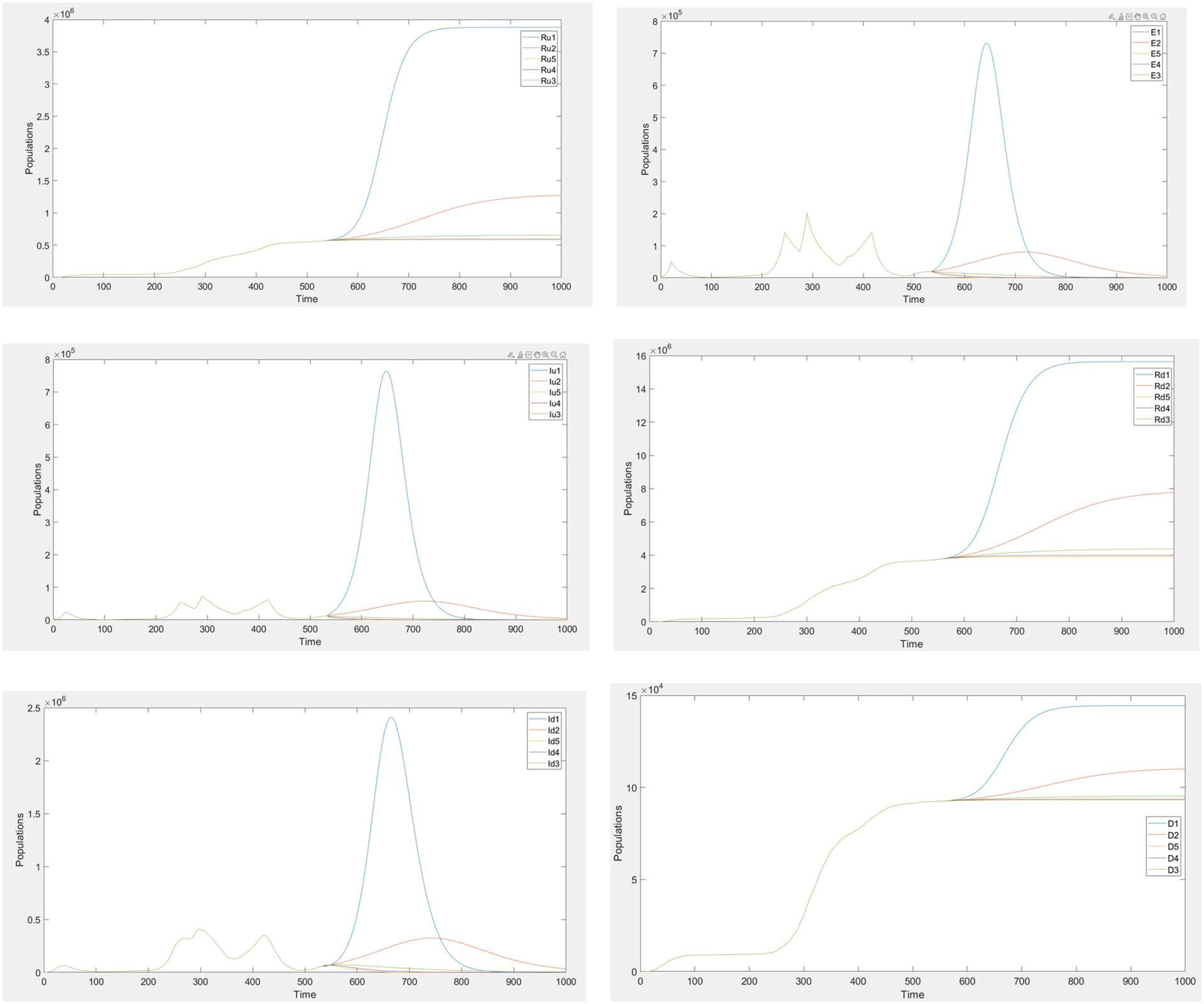
The model’s sensitivity to parameter variations was analyzed over 467 days, starting from day 534 where the retrospective analysis ends, until day 1001. Parameters that were chosen to be analyzed were transmission rates a₁ and a₂, which also affect transmission rates of alpha and delta variants a₃, a₄, a₅, a₆, and detection rate q. Recovery rates g_D, g_W, which also affects g_A; mortality rates m_W, which also affects m_A, and m_D were also analyzed. The multiplicative factors were arbitrarily chosen to be 0.5, 0.8, 1, 1.2, and 1.5 to show an extended range of variations. The compartments that the effects of the parameter variations were analyzed on are: total exposed (E_W+E_A+E_D), currently undetected infected (I_UW+I_UA+I_UD), currently detected infected (I_DW+I_DA+I_DD), undetected recovered R_U, detected recovered R_D, deceased D. Since we only consider the Vaccinated compartment to replicate the real data, we do not analyze it after the final day, 534. That is why the Vaccinated compartment was not included in the sensitivity analysis, further vaccinations are ignored.

Figure 6:

Currently infected population data vs. the model.

Figure 7:

Cumulative detected infected population data vs. the model.

Figure 8:

Cumulative total infected population data vs. the model (including the undetected compartments).

Figure 9:

Competition between the infected compartments of SARS-CoV-2 strains wild-type, alpha, and delta.

Sensitivity analysis of a₁ and a₂

Increasing the transmission rate parameters results in the increase of undetected recovered, detected recovered, and deceased compartments. Multiplying the transmission rates by 1.5 causes a higher peak to occur in total exposed, total undetected infected, and total detected infected compartments, which then quickly decreases towards zero. Multiplying by 1.2 causes a lower peak to occur in the same compartments, which then slowly decreases towards zero. Decreasing the same parameters results in the decrease of the same compartments (Extended Data Figures 1 and 2).

Sensitivity analysis of q

Decreasing the detection rate parameter results in the increase of undetected recovered, detected recovered, and deceased compartments. Multiplying the detection rate by 0.5 causes a higher peak to occur in total exposed, total undetected infected, and total detected infected compartments, which then quickly decreases towards zero. Multiplying by 0.8 causes a lower peak to occur in the same compartments, which then slowly decreases towards zero. Increasing the same parameter results in the decrease of the same compartments (Extended Data Figure 3).

Sensitivity analysis of g_W and g_A

All the analyzed compartments are found to be not sensitive to the changes in the recovery rate parameters of wild-type and alpha strains, since by the final day 534, they are replaced by the delta variant and nearly extinct (Extended Data Figure 4).

Sensitivity analysis of g_D

Decreasing the recovery rate parameter of the delta variant results in the increase of the total exposed, total undetected infected, and total detected infected compartments. Increasing the same parameter increases the detected and undetected recovered compartments initially, to decrease afterwards compared to other multiplicative factors. Decreasing the same parameter results in an increase in the deceased compartment (Extended Data Figure 5).

Sensitivity analysis of m_W and m_A and m_D

Mortality rate parameters are found to be only meaningfully affecting the deceased compartment. Increasing the mortality rate parameters increases the deceased compartment (Extended Data Figure 6).

Alternative vaccination scenario analysis

Below, the impact of non-existent, imperfect, and accelerated vaccination administration is examined using multipliers that have been arbitrarily chosen. These multipliers have been selected to be 0, 0.5, and 1.5 to demonstrate a wide range of variations. The analysis considers the effects on several compartments, including currently detected infected (I_DW+I_DA+I_DD), detected recovered R_D, deceased D, cumulative detected infected (I_DW+I_DA+I_DD+R_D +D), and cumulative total infected (I_DW+I_DA+I_DD+R_D +D+I_UW+I_UA+I_UD+R_U). The analysis kept the interval conditions the same as before, and only the vaccination rate was altered. It’s important to note that this analysis may not be entirely realistic since regulations did not adjust according to the severity of the pandemic. Consequently, if the vaccination rate were lower, regulators would likely have enforced more stringent measures.

Imperfect vaccination

At the end of the analysis, the number of individuals in the deceased compartment was 91,927. However, this number increased to 128,379 under the imperfect vaccination condition. The currently detected infected compartment size showed a significant increase in the final interval, and both cumulative detected and total infected compartment sizes also increased significantly under this circumstance. In the imperfect vaccination scenario, the size of the detected recovered compartment increased, which may be attributed to the increase in the size of the infected compartments (Extended Data Figure 7).

Non-existent vaccination

At the conclusion of the analysis, the number of individuals in the deceased compartment was 91,927. However, if there had been no vaccination administration, our simulation predicted this number would have been much higher, at 472,798. The currently detected infected compartment initially increased, but then began to decrease, likely due to increased population immunity resulting from a decrease in the susceptible compartment. Under the scenario where there is no vaccination, both cumulative detected infected and cumulative total infected compartments showed a significant increase, along with the detected recovered compartment (Extended Data Figure 8).

Accelerated vaccination

The analysis of the accelerated vaccination scenario showed that there were minimal new deaths compared to the non-existent and imperfect vaccination simulations, resulting in a relatively stable size for the deceased compartment. Moreover, the currently detected infected compartment plummeted in the final interval of the analysis. Although both the cumulative detected infected and detected recovered compartments remained below the real data, the cumulative total infected compartment stayed above the real data. This was because the cumulative total infected compartment accounted for undetected infected individuals, highlighting the importance of considering this group in understanding the true impact of the pandemic (Extended Data Figure 9).

Discussion and conclusions

In this paper, we propose a novel deterministic compartmental model including the dynamics of vaccination, the three most common strains of the virus (wild-type, alpha, and delta), the detection status of infected individuals and pre-symptomatic transmission that represents the pandemic course in Germany between the dates of 02.03.2020 and 17.08.2021. With this model, we analyzed the behavior of the German population in 534 days, 25 time intervals, and estimated the values of the parameters in each interval such as transmission, recovery, mortality, and detection. We used a set of nonlinear ordinary differential equations to model the COVID-19 disease. For the numerical solution of this model, we used Runge-Kutta 4 method. After manually estimating the parameter values, we used the LSQNONLIN function to optimize the parameters. All is coded in MATLAB.

To control the contagion, authorities should quantitatively know how the pandemic course would change under different circumstances. To achieve this information, it is crucial to analyze an extensive time scale of the pandemic, which is why we present an analysis of 534 days. This analysis provides an extended range of circumstances and respective parameters that can also be applied to future scenarios which can be simulated by policymakers.

This model does not categorize infected individuals based on the severity of their symptoms but rather on whether they have been diagnosed by a medical authority. This approach is favored because the transmission coefficients are determined by whether the patient is diagnosed or not, which affects their ability to transmit the disease. Additionally, this categorization allows for the detection of asymptomatic individuals, which can help lower their transmission rate, and accounts for the possibility of authorities missing mildly symptomatic individuals, which could increase their transmission rate. Despite potential criticisms that a more detailed approach considering both symptoms and detection could be more accurate, this model prioritizes convenience by reducing complexity and allowing for other important compartments such as vaccinated individuals and separate compartments for different virus strains.

An alternative analysis of vaccination under the same interval conditions suggests that less-than-perfect vaccination could have catastrophic consequences. In the case of imperfect vaccination, the size of the deceased compartment increased to a lesser extent compared to the non-existent vaccination scenario. However, both scenarios resulted in a significant increase in the currently detected infected compartment towards the end of the simulation, which could lead to a sustained increase in the death toll even beyond the simulated time course. Conversely, under accelerated vaccination conditions, if vaccines had been more accessible and vaccination awareness had been more widespread in society, the number of currently infected individuals would have decreased rapidly, leading to a decrease in the number of deaths and eventually resulting in earlier relief from the COVID-19 pandemic course in Germany.

The model developed in this paper has several shortcomings that need to be addressed. For instance, the model does not account for re-infections and immunity wane, which means that there is no population flow to the susceptible compartment from the recovered and vaccinated compartments. Despite these limitations, the model provides a general infrastructure that can be further improved by adding future variants of concern or incorporating other factors that may impact the dynamics of the pandemic.

Corresponding author: Çağan Kaplan, Faculty of Medicine, Ege University, Bornova 35100, İzmir, Türkiye, E-mail: cagan.kaplan@hotmail.com

Yıldırım Adalıoğlu and Çağan Kaplan contributed equally to this work.

Research funding: None declared.
Author contributions: All authors have accepted responsibility for the entire content of this manuscript and approved its submission.
Competing interests: Authors state no conflict of interest.
Informed consent: Not applicable.
Ethical approval: Not applicable.

Appendix

Extended Data Figure 1

Extended Data Figure 2

Extended Data Figure 3

Extended Data Figure 4

Extended Data Figure 5

Extended Data Figure 6

Extended Data Figure 7

Extended Data Figure 8

Extended Data Figure 9

References

6. Mai 2020: Regeln zum Corona-Virus . n.d. Die Bundesregierung Informiert | Startseite. https://www.bundesregierung.de/breg-de/leichte-sprache/6-mai-2020-regeln-zum-corona-virus-1755252.Search in Google Scholar

Aus Reisewarnung wird Reisehinweis . 2020. Die Bundesregierung Informiert | Startseite. https://www.bundesregierung.de/breg-de/themen/coronavirus/reisen-wieder-moeglich-1757372.Search in Google Scholar

Barbarossa, M. V., J. Fuhrmann, J. H. Meinke, S. Krieg, H. V. Varma, N. Castelletti, and T. Lippert. 2020. “Modeling the Spread of COVID-19 in Germany: Early Assessment and Possible Scenarios.” PLoS One 15 (9): e0238559. https://doi.org/10.1371/journal.pone.0238559.Search in Google Scholar PubMed PubMed Central

Besprechung der Bundeskanzlerin mit den Regierungschefinnen und Regierungschefs der Länder vom 22.03.2020. 2020. Die Bundesregierung Informiert | Startseite. https://www.bundesregierung.de/breg-de/themen/coronavirus/besprechung-der-bundeskanzlerin-mit-den-regierungschefinnen-und-regierungschefs-der-laender-vom-22-03-2020-1733248.Search in Google Scholar

Bund-Länder-Verständigung Corona-Maßnahmen . 2020. Die Bundesregierung Informiert | Startseite. https://www.bundesregierung.de/breg-de/themen/coronavirus/fahrplan-corona-pandemie-1744202.Search in Google Scholar

Bulfone, T. C., M. Malekinejad, G. W. Rutherford, and N. Razani. 2020. “Outdoor Transmission of SARS-CoV-2 and Other Respiratory Viruses: A Systematic Review.” The Journal of Infectious Diseases 223 (4): 550–61. https://doi.org/10.1093/infdis/jiaa742.Search in Google Scholar PubMed PubMed Central

Bund und Länder beschließen stufenweise Lockerungen . 2021. Die Bundesregierung Informiert | Startseite. https://www.bundesregierung.de/breg-de/themen/coronavirus/bund-laender-beschluss-1872126.Search in Google Scholar

Chronik zum Coronavirus SARS-CoV-2 . n.d. Chronik Zum Coronavirus SARS-CoV-2 | Maßnahmen. https://www.bundesgesundheitsministerium.de/coronavirus/chronik-coronavirus.html.Search in Google Scholar

Corona: Indien wird als Virusvarianten-Gebiet eingestuft . 2021. Die Bundesregierung Informiert | Startseite. https://www.bundesregierung.de/breg-de/suche/corona-indien-virusvarianten-gebiet-1897514.Search in Google Scholar

Corona-Schutzmaßnahmen: Erleichterungen für Geimpfte und Genesene . 2021. Die Bundesregierung Informiert | Startseite. https://www.bundesregierung.de/breg-de/themen/coronavirus/erleichterungen-geimpfte-1910886.Search in Google Scholar

Coronavirus: Regeln in den Bundesländern | Bundesregierung . n.d. Die Bundesregierung Informiert | Startseite. https://www.bundesregierung.de/breg-de/themen/coronavirus/corona-bundeslaender-1745198.Search in Google Scholar

Coronavirus-Schutzverordnung – CoronaSchV (Englisch) . n.d. Coronavirus-Schutzverordnung – CoronaSchV (Englisch). https://www.bundesgesundheitsministerium.de/service/gesetze-und-verordnungen/guv-19-lp/coronaschv/coronaschv-en.html.Search in Google Scholar

Deutschlands Informationsplattform zum Coronavirus . n.d. https://www.zusammengegencorona.de/faqs/covid-19/quarantaene-und-isolierung/#:∼:text=Enge%20Kontaktpersonen%20sollten%20sich%20bereits,Kontakte%20au%C3%9Ferhalb%20des%20Haushalts%20informieren.Search in Google Scholar

Diekmann, O., J. Heesterbeek, and M. G. Roberts. 2010. “The Construction of Next-Generation Matrices for Compartmental Epidemic Models.” Journal of The Royal Society Interface 7 (47): 873–85. https://doi.org/10.1098/rsif.2009.0386.Search in Google Scholar PubMed PubMed Central

Dong, E., H. Du, and L. Gardner. 2020. “An Interactive Web-Based Dashboard to Track COVID-19 in Real Time.” The Lancet Infectious Diseases 20 (5): 533–4. https://doi.org/10.1016/s1473-3099(20)30120-1.Search in Google Scholar

Elbe, S., and G. Buckland-Merrett. 2017. “Data, Disease and Diplomacy: GISAID’s Innovative Contribution to Global Health.” Global Challenges 1 (1): 33–46. https://doi.org/10.1002/gch2.1018.Search in Google Scholar PubMed PubMed Central

Evensen, G., J. Amezcua, M. Bocquet, A. Carrassi, A. Farchi, A. Fowler, P. L. Houtekamer, C. W. Jones, R. J. De Moraes, M. L. Pulido, C. E. Sampson, and F. C. Vossepoel. 2020. “An International Assessment of the COVID-19 Pandemic Using Ensemble Data Assimilation.” medRxiv. https://doi.org/10.1101/2020.06.11.20128777.Search in Google Scholar

FAQ on the New Protection Against Infections Act . n.d. FAQ on the New Protection Against Infections Act. https://www.bundesgesundheitsministerium.de/service/gesetze-und-verordnungen/guv-19-lp/4-bevschg-faq/faq-infections-act.html.Search in Google Scholar

Federal and State Governments Extend COVID-19 Measures Until 14 February . 2021. Website of the Federal Government | Bundesregierung. https://www.bundesregierung.de/breg-en/service/archive/decision-of-federal-and-state-governments-1841104.Search in Google Scholar

Fisman, D. N., and A. R. Tuite. 2021. “Evaluation of the Relative Virulence of Novel SARS-CoV-2 Variants: A Retrospective Cohort Study in Ontario, Canada.” Canadian Medical Association Journal 193 (42): E1619–25. https://doi.org/10.1503/cmaj.211248.Search in Google Scholar PubMed PubMed Central

Ghostine, R., M. E. Gharamti, S. Hassrouny, and I. Hoteit. 2021. “An Extended SEIR Model with Vaccination for Forecasting the COVID-19 Pandemic in Saudi Arabia Using an Ensemble Kalman Filter.” Mathematics 9 (6): 636. https://doi.org/10.3390/math9060636.Search in Google Scholar

Giordano, G., F. Blanchini, R. Bruno, P. Colaneri, A. Di Filippo, A. Di Matteo, and M. Colaneri. 2020. “Modelling the COVID-19 Epidemic and Implementation of Population-wide Interventions in Italy.” Nature Medicine 26 (6): 855–60. https://doi.org/10.1038/s41591-020-0883-7.Search in Google Scholar PubMed PubMed Central

Grant, R., T. Charmet, L. Schaeffer, S. Galmiche, Y. Madec, C. Von Platen, O. Chény, F. Omar, C. David, A. Rogoff, J. Paireau, S. Cauchemez, F. Carrat, A. Septfons, D. Lévy-Bruhl, A. Mailles, and A. Fontanet. 2021. “Impact of SARS-CoV-2 Delta Variant on Incubation, Transmission Settings and Vaccine Effectiveness: Results from a Nationwide Case-Control Study in France.” The Lancet Regional Health 13: 100278. https://doi.org/10.1016/j.lanepe.2021.100278.Search in Google Scholar PubMed PubMed Central

Infection Protection Act – Nationwide Emergency Brake . 2021. Website of the Federal Government | Bundesregierung. https://www.bundesregierung.de/breg-en/service/archive/nationwide-emergency-brake-1889136.Search in Google Scholar

Khare, S., C. Gurry, L. C. Freitas, M. B. Schultz, G. Bach, A. S. Diallo, N. Akite, J. Ho, R. C. Lee, W. Yeo, G. C. C. Team, and S. Maurer-Stroh. 2021. “GISAID’s Role in Pandemic Response.” China CDC Weekly 3 (49): 1049–51. https://doi.org/10.46234/ccdcw2021.255.Search in Google Scholar PubMed PubMed Central

Kraemer, M. U. G., V. Hill, C. Ruis, S. Dellicour, S. Bajaj, J. T. McCrone, G. Baele, K. V. Parag, A. L. Battle, B. Gutierrez, B. Jackson, R. M. Colquhoun, Á. O’Toole, B. Klein, A. Vespignani, E. M. Volz, N. R. Faria, D. M. Aanensen, N. J. Loman, O. G. Pybus, S. Cauchemez, A. Rambaut, and S. V. Scarpino. 2021. “Spatiotemporal Invasion Dynamics of SARS-CoV-2 Lineage B.1.1.7 Emergence.” Science 373 (6557): 889–95. https://doi.org/10.1126/science.abj0113.Search in Google Scholar PubMed PubMed Central

MATLAB Curve Fitting Toolbox, 3.6. 2021. https://www.mathworks.com/products/curvefitting.html.Search in Google Scholar

MATLAB Optimization Toolbox, 9.2. 2021. https://www.mathworks.com/products/optimization.html.Search in Google Scholar

Moore, C. X., R. Sergienko, and R. Arbel. 2021. “SARS-CoV-2 Alpha Variant: Is it Really More Deadly? A Population Level Observational Study.” medRxiv. https://doi.org/10.1101/2021.08.17.21262167.Search in Google Scholar

Ritchie, H., E. Mathieu, L. Rodés-Guirao, C. Appel, C. Giattino, E. Ortiz-Ospina, J. Hasell, B. Macdonald, D. Beltekian and M. Roser. 2020. “Coronavirus Pandemic (COVID-19).” OurWorldInData.org. https://ourworldindata.org/coronavirus.Search in Google Scholar

Rowe, B., A. Canosa, J. Drouffe, and J. Mitchell. 2021. “Simple Quantitative Assessment of the Outdoor versus Indoor Airborne Transmission of Viruses and COVID-19.” Environmental Research 198: 111189. https://doi.org/10.1016/j.envres.2021.111189.Search in Google Scholar PubMed PubMed Central

Scientific Advisory Group for Emergencies. 2021. SPI-M-O: Consensus statement on COVID-19, 3 June 2021. GOV.UK. https://www.gov.uk/government/publications/spi-m-o-consensus-statement-on-covid-19-3-june-2021.Search in Google Scholar

Shu, Y., and J. W. McCauley. 2017. “GISAID: Global Initiative on Sharing All Influenza Data – from Vision to Reality.” Euro Surveillance 22 (13). https://doi.org/10.2807/1560-7917.es.2017.22.13.30494.Search in Google Scholar

Testpflicht für ungeimpfte Reiserückkehrer. 2021. Die Bundesregierung Informiert | Startseite. https://www.bundesregierung.de/breg-de/suche/testpflicht-reiserueckkehrer-1772096.Search in Google Scholar

Tong, Z., A. Tang, K. Li, P. Li, H. Wang, J. Yi, Y. Zhang, and J. Yan. 2020. “Potential Presymptomatic Transmission of SARS-CoV-2, Zhejiang Province, China, 2020.” Emerging Infectious Diseases 26 (5): 1052–4. https://doi.org/10.3201/eid2605.200198.Search in Google Scholar PubMed PubMed Central

United Nations, Department of Economic and Social Affairs, Population Division. 2019. World Population Prospects 2019, Online Edition. Rev. 1.Search in Google Scholar

Van Den Driessche, P., and J. Watmough. 2002. “Reproduction Numbers and Sub-threshold Endemic Equilibria for Compartmental Models of Disease Transmission.” Mathematical Biosciences 180 (1–2): 29–48. https://doi.org/10.1016/s0025-5564(02)00108-6.Search in Google Scholar PubMed

Velavan, T. P., and C. Meyer. 2020. “The COVID‐19 Epidemic.” Tropical Medicine and International Health 25 (3): 278–80. https://doi.org/10.1111/tmi.13383.Search in Google Scholar PubMed PubMed Central

Wir sind zum Handeln gezwungen . 2021. Die Bundesregierung Informiert | Startseite. https://www.bundesregierung.de/breg-de/themen/coronavirus/merkel-beschluss-weihnachten-1827396.Search in Google Scholar

Worldometers.info. 2022. Recoveries [Data Set]. Dover. https://www.worldometers.info/coronavirus/country/germany/.Search in Google Scholar

Wu, Z., and J. M. McGoogan. 2020. “Characteristics of and Important Lessons from the Coronavirus Disease 2019 (COVID-19) Outbreak in China.” JAMA 323 (13): 1239. https://doi.org/10.1001/jama.2020.2648.Search in Google Scholar PubMed

Yu, P., J. Zhu, Z. Zhang, and Y. Han. 2020. “A Familial Cluster of Infection Associated with the 2019 Novel Coronavirus Indicating Possible Person-To-Person Transmission during the Incubation Period.” The Journal of Infectious Diseases 221 (11): 1757–61. https://doi.org/10.1093/infdis/jiaa077.Search in Google Scholar PubMed PubMed Central

Received: 2022-07-17

Accepted: 2023-05-29

Published Online: 2023-06-29

Articles in the same Issue

https://doi.org/10.1515/em-2022-0126

Keywords for this article

compartmental models; computational epidemiology; COVID-19; extended SEIR models; Germany

A compartmental model of the COVID-19 pandemic course in Germany

Article

Abstract

Objectives

Methods

Results

Conclusions

Introduction

Methods

Model

Equation system

Mathematical analysis of the model

Non-negativity of the model

Proposition

Proof

Boundness of the model

Computation of Rt

Numerical analysis

Course of the pandemic

Results

Model simulation compared to real data

Sensitivity analysis

Sensitivity analysis of a1 and a2

Sensitivity analysis of q

Sensitivity analysis of gW and gA

Sensitivity analysis of gD

Sensitivity analysis of mW and mA and mD

Alternative vaccination scenario analysis

Imperfect vaccination

Non-existent vaccination

Accelerated vaccination

Discussion and conclusions

Extended Data Figure 1

Extended Data Figure 2

Extended Data Figure 3

Extended Data Figure 4

Extended Data Figure 5

Extended Data Figure 6

Extended Data Figure 7

Extended Data Figure 8

Extended Data Figure 9

References

Articles in the same Issue

Articles in the same Issue

Articles in the same Issue

Computation of R_t

Sensitivity analysis of a₁ and a₂

Sensitivity analysis of g_W and g_A

Sensitivity analysis of g_D

Sensitivity analysis of m_W and m_A and m_D