Identification of time delays in COVID-19 data
-
Nicola Guglielmi

 and
Alex Viguerie
and
Alex Viguerie

Abstract
Objective
COVID-19 data released by public health authorities is subject to inherent time delays. Such delays have many causes, including delays in data reporting and the natural incubation period of the disease. We develop and introduce a numerical procedure to recover the distribution of these delays from data.
Methods
We extend a previously-introduced compartmental model with a nonlinear, distributed-delay term with a general distribution, obtaining an integrodifferential equation. We show this model can be approximated by a weighted-sum of constant time-delay terms, yielding a linear problem for the distribution weights. Standard optimization can then be used to recover the weights, approximating the distribution of the time delays. We demonstrate the viability of the approach against data from Italy and Austria.
Results
We find that the delay-distributions for both Italy and Austria follow a Gaussian-like profile, with a mean of around 11 to 14 days. However, we note that the delay does not appear constant across all data types, with infection, recovery, and mortality data showing slightly different trends, suggesting the presence of independent delays in each of these processes. We also found that the recovered delay-distribution is not sensitive to the discretization resolution.
Conclusions
These results establish the validity of the introduced procedure for the identification of time-delays in COVID-19 data. Our methods are not limited to COVID-19, and may be applied to other types of epidemiological data, or indeed any dynamical system with time-delay effects.
Introduction
The outbreak of COVID-19 in 2020 and into 2021 has led to a surge in interest in the mathematical modeling of the COVID-19 epidemic, as well as the mathematical modeling of epidemics generally. These models have taken many types. A full review of the relevant literature is beyond the current work. However, some general classes of models include data-driven and machine learning approaches (Barros et al. 2022; Bhouri et al. 2021; Jha, Cao, and Oden 2020; Linka et al. 2020; Viguerie et al. 2022a; Wang et al. 2020), models based on partial differential equation (PDE) systems (Albi et al. 2022; Bertaglia and Pareschi 2021a,b; Bertrand and Pirch 2021; Grave et al. 2021; Grave and Coutinho 2021; Viguerie et al. 2020, 2021), agent-based models (Zohdi 2020), and models based on ordinary differential equation (ODE) systems. This last category is by far the most common, with such articles numbering in the thousands. Some works of this type include e.g. (Calafiore, Novara, and Possieri 2020; Choi and Ki 2020; Ferguson et al. 2020; Gatto et al. 2020; Ivorra et al. 2020; Parolini et al. 2021; Piccolomini and Zama 2020; Remuzzi and Remuzzi 2020). We note that the categories listed above are not necessarily strict delimiters; indeed, many of the above cited works, as well myriad others, have characteristics of multiple of different model classes. One commonality that nearly all the presented models share is that they are, in some way, compartmental models in the SIR family owing to the seminal work of Kermack and Mackendrick (Ogilvy Kermack and McKendrick 1927) (see also: Breda et al. 2012; Murray 2007; Iannelli and Pugliese 2015).
One of the most important aspects of COVID-19 modeling, and epidemiological modeling in general deals with the presence of time delays in the data. Time delays certainly manifest themselves via the natural incubation period of the disease; this is reflected in the employed models commonly incorporating an exposed compartment, to model the period after exposure to the virus but before symptomatic infection (Bhouri et al. 2021; Gatto et al. 2020; Linka et al. 2020; Viguerie et al. 2020) also shown in Figure 1.

Flow chart describing the evolution of the various compartments in a classical SEIRD model.
Such an approach is a reasonable one, though, there are several potential problems. First of all, the exposed compartment is not necessarily easily known from data, and hence must be estimated. This may be done, for example, through rule-of-thumb estimates based on the infected population, which result in high uncertainty (Albi et al. 2022; Grave and Coutinho 2021; Grave et al. 2021). Compounding this problem further are the well-known presence of asymptomatic patients, who may spread the disease while never showing appreciable symptoms, and, at least in the earlier stages of the pandemic, were almost certainly under-counted (Albi et al. 2022; Viguerie et al. 2020).
Another major problem with the exposed compartment in most SEIR-type formulations come from estimating the sojourn time of incubation period, or the length of time spent in the compartment. Under most common compartmental approaches, the sojourn time of the exposed period is implicitly assumed to follow an exponential distribution. In practice, this may not always be a realistic (Iannelli and Pugliese 2015) assumption.
In (Guglielmi, Iacomini, and Viguerie 2022; Viguerie et al. 2022a), the authors employed a delay-differential equation (DDE) model, in which the incubation period was modeled with a time-delay term, rather than as a separate exposed compartment. Such a modeling approach eliminated the need to estimate the exposed compartment, as well as the assumption of an exponentially-distributed sojourn time for the incubation period, instead assuming a Dirac-delta (constant) distribution. Other works incorporating DDE models into the analysis of COVID-19 include (Dell’Anna 2020; Devipriya, Dhamodharavadhani, and Selvi 2021; Kumar and Erturk 2020), while references for more general epidemiological models of this type may be found in (Brauer and Castillo-Chavez 2012; Buonomo, d’Onofrio, and Lacitignola 2008; Forde 2005; Iannelli and Pugliese 2015; Murray 2007; Takeuchi, Ma, and Beretta 2000).
Aside from the presence of incubation periods, delays in data may result from other sources: additional time from initial onset of symptoms to when a person decides to be tested, the availability of testing, the speed of test result processing, testing center capacity, and other factors may have a large influence on when a given case is properly identified in the data (Sarnaglia et al. 2021). The presence of such lags is important, particularly when attempting to model measured data, as such processes are intrinsic to the data (Bastos et al. 2019). Hence, when attempting to properly evaluate different intervention strategies, for instance, such delays must be considered in the modeling process. A model designed to fit measured parameters, while not taking into account the delays in measurement, may fail provide a wholly accurate description of the dynamics. In this sense, we may view such delays as no longer time from exposure to infection, but rather time from exposure to identification.
Quantifying both the magnitude and distribution of such time delays, considering the effects of both identification lag-time as well as the natural incubation period, is thus important for evaluating intervention efficacy and allocation of resources, and is the focus of the present work. In order to accomplish this task, we first introduce, as a forward problem, an SIRD (susceptible-infected-recovered-deceased) model, in which the time from infection to identification is not assumed to follow any particular distribution. At the continuous level, this is accomplished via a convolution with an unknown probability distribution function. We then approximate the continuous probability distribute function with a discrete approximation, reducing the convolution term to a weighted sum of constant time-delays. In this way, we obtain a linear problem in terms of the distribution weights, enabling us to employ an optimization procedure against measured data to identify the weights, thus approximating the distribution of the time delays present in the data. We note that the introduced method, while applied in the current work to COVID-19, is general in nature and such a technique may be employed in any situation in which a dynamical system and its associated measurements may exhibit time-delayed dynamics whose distribution is not known.
The article is outlined as follows. We first introduce the employed delay-differential equation model and discuss some of its characteristics at the continuous level. We then introduce its discrete analogue and describe the optimization process for the identification of the time delay distribution. We then validate the proposed technique on an interval of data for the COVID-19 outbreaks in Italy and Austria demonstrating its effectiveness for different cases under different modeling assumptions. Finally, we conclude with a summary of our main findings and possible directions for future research in this area.
Delay differential equation model
The delay differential model introduced in (Guglielmi, Iacomini, and Viguerie 2022) reads as follows:
Here, s(t), i(t), r(t), d(t) represent respectively the susceptible, infected, recovered and deceased compartments at time t. The parameter σ represents the time delay term which models the incubation period of the disease, as well as potential reporting delays. For a comprehensive description of the parameters and variables of the model, with the units of measure, we refer to Table 1. Moreover the living population is given by n = s + i + r + d.
Relevant parameters and variables, with symbols and unit of measure. Note that s, i, r, d are the variables of the system, while the others are parameters.
| Parameter/variable | Name | Units |
|---|---|---|
| s | Susceptible individuals | Persons |
| i | Infected individuals | Persons |
| r | Recovered individuals | Persons |
| d | Deceased individuals | Persons |
| β | Contact rate | Persons−1 ⋅ Days−1 |
| ϕ r | Recovery rate | Days−1 |
| ϕ d | Mortality rate | Days−1 |
| σ j , j = 1: k | Time-delay j | Days |
| w j , j = 1: k | Time-delay weight j | Dimensionless |
We assume the following:
That the time scales considered are sufficiently short such that we do not need to consider new births or non-COVID-19 deaths;
That the population is sufficiently well-mixed in space, such that spatial dynamics (including the Allee effect on the transmission terms, see Viguerie et al. 2021) can be ignored;
That the time scales considered are sufficiently short such that we do not need to consider waning immunity;
That recovery and mortality rates follow an exponential distribution;
That the model depends on time-delays, arising from both natural (incubation period) and non-natural (measurement and reporting delays, and similar) causes, whose distribution is unknown.
where σ min and σ max denote the extrema of the time delays. Note that the presence of the convolution term:
where w(σ) ≥ 0 is a probability density function describing the distribution of the time-delay dependence present in the model. By definition,
Under the assumption (with δ(⋅) a Dirac-δ distribution):
for a certain constant
The function w is unknown in general, and its identification in terms of the available measured data is the focus of the present work. To render the problem numerically tractable, we replace w(σ) in (5)–(8) with a piecewise-constant approximation, letting {σ
j
} denote a partition of the interval, assumed uniform for simplicity:
where the χ j are simple functions, defined such that:
From the mean value theorem, for each [σ
j−1, σ
j
), there exists a
We then define the
We then have:
where the final line follows from the simple approximation:
Hence, by defining
we obtain the approximation:
Note that:
To see this, observe from (14), (18):
From the preceding arguments, (16), replacing w(σ) in (5)–(8) with its piecewise approximation (12) gives the following system of ordinary delayed-differential equations:
It was shown in (Guglielmi, Iacomini, and Viguerie 2022) that, for k = 1 (and thus only one time-delay
which, for the more general case, easily extends to:
for each j.
The significance of replacing (5)–(8) with the above approximation (22)–(25) is that we now have a problem which is linear in w j . This allows us to make use of an optimization procedure to identify the w j , allowing us to estimate w(σ). Therefore, we are able to numerically estimate the dependence of the data on general time-delays, assuming only that w(σ) is sufficiently smooth over the relevant interval. In contrast, many common modeling approaches assume, for example, that such delays are exponentially distributed (as in most standard compartment models), or that the delays are constant (as in most basic delay-differential equation models). We remark while we consider only distributions ω assumed to not vary in time in the present work, the above framework can nonetheless accommodate time-dependent ω, provided that such time-dependence is sufficiently smooth.
Optimization procedure and methods
Denote the measured susceptible, infected, recovered, and deceased (from COVID-19) populations as
subject to
The novelty of the proposed method above lies in the approximation (12) of w(σ), allowing us to consider the nonlinear convolution term (9) as a weighted sum of constant-delay terms. Through this approximation, it is possible to obtain an optimization problem for the time delay that is linear in w j . This is important, as attempting to optimize for w(σ) directly on (5)–(8) gives a highly nonlinear optimization problem that is likely untractable. This method of identifying a general distribution by approximating it as a weighted sum of constant time delays, then solving an optimization problem for the weights is, to the authors’ knowledge, novel. We note that this approach is highly general and is not restricted to models of COVID-19 or epidemiological models in general. Indeed, one may use an analogous approach to identify general sojourn times in compartmental models. Moreover, the accuracy and the detailed description of the delay depend on how k is chosen. This allows this method to be very applicable for other models as well.
We note that the model (22)–(25) depends heavily not only on the approximate delay-distribution w j , but also on the contact rate β, recovery rate ϕ r , and mortality rate ϕ d . These parameters are also, in general, not known. In order to obtain more robust estimates for the w j through the optimization procedure defined above, we resort to a Monte Carlo method. The idea of this class of algorithms is to repeat random sample from the distribution function of the random variable, and perform several runs of the simulation, one for each sample. The solution will be given by the mean of all the obtained result. For a detailed description of Monte-Carlo methods we refer to (Pareschi and Toscani 2013).
Here, the Monte Carlo method consists of considering the β, ϕ r , ϕ d as independent random variables sampled from a Gaussian distributions. The mean of the respective distributions is obtained via an empirical parameter fitting, with the standard deviation of each distribution taken to be 5 % the value of the mean. This value was chosen based on sensitivity analyses. We then run the optimization procedure (28a)–(28c) a total of 1,000 times, corresponding to 1,000 different parameter samplings. We then identify frequency with which different w j appear in the optimization, as well as the mean value of each w j over the sampled trial.
We note that the result optimization procedure (16a)–(16d) depends on the choice of input data. In general, we consider the infection and deceased data to be the most reliable such data and is emphasized in our calculations. As the easiest quantity to measure, the deceased compartment is assumed the most accurate. Further, the as the rate of new infections is the driving point behind policy measures, it is considered the second most accurate measure for our purposes. However, one may modify (16a) to include other compartments, or different subsets of the compartment set.
In terms of implementation, there are several important points to note. We define the optimization procedure using the MATLAB routine fmincon. In order to solve the delay differential equation system (22)–(25), we use the MATLAB function dde23. We note that dde23 uses adaptive grid points, and hence the temporal points of the solution obtained using dde23 do not correspond to those in our dataset in general. To circumvent this, we use deval to evaluate the dde23 solution at the desired temporal points.
Results
For our measured data, we consider the second wave of COVID-19 outbreak in Italy and Austria, as reported by the newspaper Il Sole 24 ORE (Coronavirus 2021) and AGES[1] respectively. The choice of these two Countries is mainly due to the availability of data as current number of positive cases and daily updates on recovered people, which was the most difficult data to find.
We consider the dates ranging from September 11, 2020 to February 7, 2021. This date range was chosen to represent a 150-day span, in which different governmental policies were enacted, widespread testing was available, and before large-scale population vaccination. This choice was intentional, as we wish to avoid as many confounding factors as possible.
Italy
We consider the following distributions for the parameters
where N(μ, ς) denotes a normal distribution with mean μ and standard distribution ς and n 0 denotes the initial living population. For t > 73,[2] where t 0 = 0, we replace β by β/3 to model the introduced government restrictions, designed to curb the virus spread. The values of ϕ d and ϕ r remain unchanged throughout the considered interval. The mean values of these parameters were obtained via a preliminary parameter tuning. For the delays, we considered 12 possible values, from σ = 2 days to σ = 35 days, with 3 days of spacing between the different days. We also performed some experiments (not shown) using different discretizations over the same range (for instance, 10 possible values) to show the robustness of the optimization procedure, which did not appreciably change the conclusions drawn.
To examine the possible differences in delays among the different compartments, we perform the optimization four times: once considering the i and d compartments together in the objective function, and for the i, r and d compartments, considering each compartment individually. For each ensemble, we report the minimum, maximum, and mean L 2 error over the simulation ensemble when compared to the measured data, as well as the mean value and frequency of the different weights w j corresponding to the delays σ j .
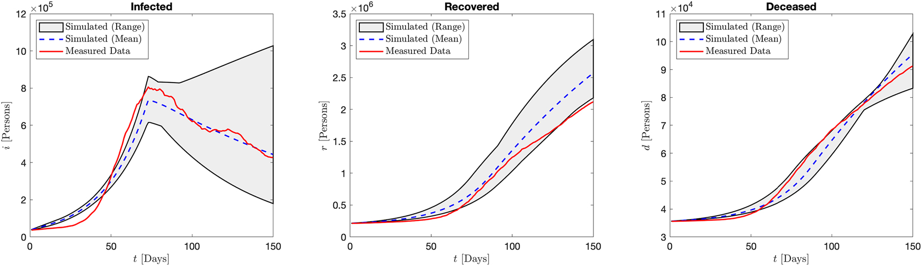
The aggregated results of the simulations in terms of the infected, recovered, and deceased compartments, when optimizing over the i and d compartments are shown in Figure 2. We see good qualitative agreement with the measured and simulated data across the three compartments of interest, with the major relevant trends being captured. In Table 2, we report the mean, minimum, and maximum of each error value computed over the simulation ensemble. We see particularly strong agreement in the susceptible and deceased compartments, reasonable agreement in the infected compartment (especially considering its rapid-changing trajectory), and somewhat worse performance in the recovered compartment. Given that the r compartment was not included in the optimization, this is unsurprising.

Italy: Aggregated results of the infected, recovered, and deceased compartments over the range of simulations when optimizing over the i and d compartments. We see good agreement across all compartments with the measured data, and particularly strong agreement (less than 10 % in L 2 norm) in the deceased compartment.
Table of relative errors in L 2 norm against measured data for the different compartments over 1,000 simulations. The compartment towards which the optimization procedure is ran is shown in the columns.
| Optim. wrt i, d | Optim. wrt i | Optim. wrt r | Optim. wrt d | ||
|---|---|---|---|---|---|
|
|
Mean | 0.0051 | 0.0051 | 0.0025 | 0.0035 |
| Min | 0.0022 | 0.0022 | 0.0016 | 0.0009 | |
| Max | 0.0104 | 0.0108 | 0.0041 | 0.0079 | |
|
|
Mean | 0.1101 | 0.1116 | 0.2347 | 0.1464 |
| Min | 0.0798 | 0.0807 | 0.1580 | 0.0826 | |
| Max | 0.2757 | 0.2681 | 0.4672 | 0.4992 | |
|
|
Mean | 0.2602 | 0.2561 | 0.0586 | 0.1903 |
| Min | 0.071 | 0.0650 | 0.0394 | 0.0440 | |
| Max | 0.5913 | 0.6054 | 0.1091 | 0.4769 | |
|
|
Mean | 0.0695 | 0.0684 | 0.0926 | 0.0430 |
| Min | 0.0249 | 0.0266 | 0.0362 | 0.0170 | |
| Max | 0.2063 | 0.1659 | 0.1672 | 0.0864 |
Turning our attention to the influence of time delays, we report the mean and frequency of the different weights w j in Figure 3. We see a heavy concentration of weights values, for both frequency and mean, in the range of σ = 8 to σ = 17 days. This is consistent with what has been reported in general media, as the incubation period of COVID is believed to have an average of 3–11 days (Byrne et al. 2020; Lauer et al. 2020; McAloon et al. 2020). When combined with natural delays coming from the testing and data reporting, a total time lag in the range of 8–17 days would appear consistent with this information.

Italy: Left: the different values of the w j by frequency of occurrence when optimizing over i and d. We see a strong concentration of weights in the range of σ = 8 to σ = 17 days. Right: the mean values of the weights over the simulation ensemble. These results mirror those of the frequency plot, showing a concentration between 8 and 17 days. For both frequency and mean, σ = 11 appears as the most represented delay.
We then repeat this experiment three more times: once each for the i, r, and d compartments considered individually in the optimization process. The error tables for the i, r and d compartments can be found in Table 2. The corresponding simulation outputs for each case are plotted in Figures 4, 6, and 8. The behavior is consistent with what one may intuitively expect; in each instance, the error behavior is minimized for the considered compartment, with the simulation variance greatly reduced for the isolated compartment. We note that one can observe from the relevant tables and figures that there is a much higher degree similarity between the i and d error behavior when compared to the r compartment, which appears to act more independently.

Italy: Aggregated results of the infected, recovered, and deceased compartments over the range of simulations when optimizing over the i compartment. We see good agreement across all compartments with the measured data, and particularly strong agreement (less than 10 % in L 2 norm) in the deceased compartment.
This is confirmed when looking at the frequency and mean distribution of the weights w j in Figures 5, 7, and 9 for the i, r, and d compartments respectively. In the case of the i compartment, we see concentration between σ = 8 and σ = 17 days, similar to when i and d are considered jointly; however, for i alone, σ = 14 appears as the most dominant lag term, rather than σ = 11. The behavior appears similar but even more pronounced when considering d alone. In this instance σ = 14 is again the dominant delay term; however, the grouping is tightly clustered between σ = 11 and σ = 17, with terms outside this range showing very little influence.

Italy: Left: the different values of the w j by frequency of occurrence when optimizing over i. We see a strong concentration of weights in the range of σ = 8 to σ = 17 days. Right: the mean values of the weights over the simulation ensemble. These results mirror those of the frequency plot, showing a concentration between 8 and 17 days. For both frequency and mean, σ = 14 appears as the most represented delay.

Italy: Aggregated results of the infected, recovered, and deceased compartments over the range of simulations when optimizing over the r compartment. We see good agreement in the r compartment; the agreement with the d compartment remains acceptable, though somewhat lesser than other optimization choices. The error in the infected compartment is notably higher. This different error behavior is reflected in the optimization results; when optimizing over r, the optimal time delays are different than when optimizing over i and d.

Italy: Left: the different values of the w j by frequency of occurrence when optimizing over r. We see a strong concentration of weights in the range of σ = 14 to σ = 20 days. Right: the mean values of the weights over the simulation ensemble. These results mirror those of the frequency plot, showing a concentration between 14 and 20 days. For both frequency and mean, σ = 17 appears as the most represented delay. These results are less similar to those obtained when one optimizes over i and d, and suggests different time-delays present in the r compartment as compared to other compartments.
Italy: Aggregated results of the infected, recovered, and deceased compartments over the range of simulations when optimizing over the d compartment. We see good agreement in the d and r compartments, with somewhat less close agreement with the i compartment.

Italy: Left: the different values of the w j by frequency of occurrence when optimizing over d. We see a tight concentration of σ in the range of 11–17 days. Right: the mean values of the weights over the simulation ensemble. These results mirror those of the frequency plot, showing a concentration between 11 and 16 days. For both frequency and mean, σ = 14 appears as the most represented delay.
In contrast, when examining the case of isolated r in 7, we see a different distribution of delay terms. Indeed, in this instance, the dominant delay terms range from σ = 14 to σ = 20, and are very tightly concentrated within this range. This suggests a distinct and longer time scale when compared to the i and d, and may explain why the error behavior for the r compartment shows a distinctly different behavior in the plots and tables shown.
Austria
We consider the following distributions for the parameters
where N(μ, ς) denotes a normal distribution with mean μ and standard distribution ς and n 0 denotes the initial living population. Note that the parameters of the random variables are different from the ones related to Italy.
For t > 66, where t 0 = 0 we replace β by β/4 to model the introduced government restrictions, namely the second hard lockdown in Austria.
As in the case of Italy, the optimization is performed four times: once considering the i and d compartments together in the objective function, and for the i, r and d compartments, considering each compartment individually. For each ensemble, we show, as before, the aggregate results of the infected, recovered and deceased compartments, the mean and the frequency of the weights w j of the delay.
Optimizing with respect to i and d, Figure 10, leads to a good agreement across all compartments with the measured data with a particular strong agreement in the deceased compartment, as in Figure 2.

Austria: Aggregated results of the infected, recovered, and deceased compartments over the range of simulations when optimizing over the i and d compartment. We see good agreement across all compartments with the measured data, and particularly strong agreement in the deceased compartment.
Concerning the weights, shown in Figure 11, both the frequency and the mean of σ are concentrated between 8 and 20 days, similar to Figure 3.

Austria: Left: the different values of the w j by frequency of occurrence when optimizing over i and d. We see a concentration of σ in the range of 8–20 days. Right: the mean values of the weights over the simulation ensemble. These results mirror those of the frequency plot, showing a concentration between 11 and 20 days. For both frequency and mean, σ = 14 appears as the most represented delay.
For the optimization with respect to the infected (Figures 12 and 13) and recovered (Figures 14, 15) compartments considered individually, we see a good agreement with the results obtained in the case of Italy, Figure 4, 5 and Figure 6, 7 respectively.

Austria: Aggregated results of the infected, recovered, and deceased compartments over the range of simulations when optimizing over the i compartment. We see good agreement across all compartments with the measured data, and particularly strong agreement in the deceased compartment.

Austria: Left: the different values of the w j by frequency of occurrence when optimizing over i. We see more σ values in the range of 11–23 days. Right: the mean values of the weights over the simulation ensemble. These results mirror those of the frequency plot, showing a concentration between 11 and 20 days. For both frequency and mean, σ = 14 appears as the most represented delay.

Austria: Aggregated results of the infected, recovered, and deceased compartments over the range of simulations when optimizing over the r compartment. We see good agreement in the r compartment; the agreement with the d compartment remains acceptable, though somewhat lower r than other optimization choices. The different error behavior is reflected in the optimization results; when optimizing over r, the optimal time delays are different than when optimizing over i and d.

Austria: Left: the different values of the w j by frequency of occurrence when optimizing over r. We see a tight concentration of σ in the range of 11–20 days. Right: the mean values of the weights over the simulation ensemble. These results mirror those of the frequency plot, showing a concentration between 11 and 16 days. For both frequency and mean, σ = 14 appears as the most represented delay These results are less similar to those obtained when one optimizes over i and d, and suggests different time-delays present in the r compartment as compared to other compartments.

Austria: Aggregated results of the infected, recovered, and deceased compartments over the range of simulations when optimizing over the d compartment. We see good agreement in the d compartment, with somewhat less close agreement with the r and i compartments.
However, this can not be said in the case of the deceased compartments (Figures 16 and 17). Here the two cases are quite different, see Figures 9 and 17. This is possibly explained by differences in how the various data are reported in the different countries causing delay distributions to differ; however, we are not sure as to the exact cause.

Austria: Left: the different values of the w j by frequency of occurrence when optimizing over d. We see a concentration of higher weights for σ in the range of 14–23 days. Right: the mean values of the weights over the simulation ensemble. These results mirror those of the frequency plot, showing a concentration between 14 and 23 days, even though the presence of sigma values also in the first and the last time-bars is notable. According to the mean value, σ = 20 appears as the most represented delay.
Sensitivity of delay distribution to discretization
In order to ensure the validity of our method, it is important to ensure that the results are insensitive to the discretization of [σ min, σ max). We perform a brief sensitivity analysis, considering the data from Austria described in the previous subsection. We consider two additional simulations, optimized over the i and d compartments (corresponding to Figures 10 and 11 above). The setup is identical to the previous simulations, except we vary the resolution of the delay discretization:
Coarse-resolution case: we discretize the interval [2, 35) with Δ = 5 days.
Fine-resolution case: we discretize the interval [2, 35) with Δ = 1 day.

Austria: Aggregated results of the infected, recovered, and deceased compartments over the range of simulations when optimizing over the i and d compartment using a coarser discretization of the delay term. The results are similar, qualitatively and quantitatively, to those obtained with a finer discretization.

Austria: Left: the different values of the w j by frequency of occurrence when optimizing over i and d when using a coarser discretization of the delay term. Right: average value of each weight over the simulation ensemble. The results are similar, qualitatively and quantitatively, to those obtained with a finer discretization.

Austria: Aggregated results of the infected, recovered, and deceased compartments over the range of simulations when optimizing over the i and d compartment using a fine discretization of the delay term. The results are similar, qualitatively and quantitatively, to those obtained with a coarser discretization.

Austria: Left: the different values of the w j by frequency of occurrence when optimizing over i and d when using a fine discretization of the delay term. Right: average value of each weight over the simulation ensemble. The results are similar, qualitatively and quantitatively, to those obtained with a coarser discretization.
In both cases, we find that the solution of the system is similar to the one obtained in the preceding section. Similarly, the delay-distributions are also similar, both qualitatively and quantitatively, compared to the previous results. From our analysis, it appears that the resolution of the delay discretization does not result in significant changes to the qualitative or quantitative profile or the identified delay distribution.
We note that increasing the resolution of the delay discretization significantly increases the computational time necessary to complete the Monte Carlo analysis. On a MacBook Pro with Processor 2 GHz, Quad-Core, Intel Core i5, with Δ = 5 (and hence 7 wt), each individual simulation required an average of 1.178 s; the average simulation instead required 3.435 s for Δ = 3 (12 wt) and 48.994 s for Δ = 1 (34 wt). Based on this evidence, it appears that one should increase the resolution of the delay term only if absolutely necessary to understand the underlying distribution, as the necessary computational cost appears to scale quadratically with the number of weights. If a coarser resolution will suffice (as appears to be the case in the present example), the significantly shorter computational time make this a more attractive choice. The authors acknowledge, however, that the optimization algorithm employed in the present work are not necessarily the most efficient choice, and that a more carefully chosen optimization algorithm may provide better scaling behavior for increasing numbers of weights.
Key-points
In all, we can conclude three key takeaway points from these results:
The time delays present in COVID-19 data range from σ = 8 to σ = 20 days, with the most likely value for σ j the i and d compartments in the range of σ = 11 to σ = 14 days, and appear to follow a normal or log-normal distribution.
The scale of the time delays across the compartments is not uniform. It is similar for new infections and for deceased persons, but occurs over a somewhat longer time scale for recovered individuals. This is not surprising due to the different recovery rate and the inherent difficulty of measuring this compartment, given delays in testing and in the reporting of results. This also suggests that the multiple delays present in the data are somewhat independent, and likely follow different distributions.
The time scales revealed by the optimization procedure shown here are longer than most estimates of the incubation period, suggesting that other delays are potentially present in the data, and a period of 14–17 days should be considered when analyzing the effects of interventions.
The results remain quantitatively and qualitatively similar when using both finer and coarser discretizations of the delay term, suggesting that the results obtained are not sensitive to this quantity.
Conclusions and future directions
In the present work, we have attempted to identify time delays present in COVID-19 data by means of newly-introduced method. This method consists of discretizing k possible time delays σ
j
, j = 1: k and expressing these terms as a weighted sum
We tested this approach on COVID-19 data in both Italy and Austria, and found that the time-delays differ among different data points, but generally speaking range between 8 and 17 days for i and d, with the most likely value between 11 and 14 days, and over a somewhat longer time scale (14–20 days) for the recovered compartment. This is consistent with our expectations given the incubation period of the disease and the natural time delays one may expect from the testing and data collection process. Our results confirm that proper evaluation of a given intervention for COVID-19 should allow for a sufficiently long time window to pass before conclusions are made. All of the identified distributions followed a bell-like distribution resembling a normal or lognormal distribution, and a sensitivity analysis suggests that this profile is independent of the discretization of the delay term.
There are several important directions for future work. Given the increased importance of waning vaccine efficacy over time, a similar analysis given vaccine data and data on breakthrough infections could be helpful in identifying similar such time-delay trends for waning immunity. While we have elected to avoid vaccines in the current work, preferring to establish a proof of concept on a more simplified problem, the approach offered is extremely general and may be applied to these important problems. Outside of COVID-19, time delays are an important part of other types of epidemiological modeling; similar methods could be used, for example, to improve back-calculation methods for estimating HIV incidence, in which incidence is estimated by reconstructing the distribution of the time-delays between infection and diagnosis (Hall et al. 2017; Song et al. 2017; Viguerie et al. 2022b; Xia et al. 2020). Further, given the generality of the proposed optimization procedure, it may have wide applications outside of epidemiology, and may be applied to any model where time delays are present, including applications in traffic modeling, pedestrian flow, remote sensing, and other fields. From the theoretical and methodological standpoint, an extension of the framework shown here for problems in which the delays are state-dependent is also an important direction of future research. Finally, we note that the general idea shown, in which general sojourn time-distributions are approximated by a weighted sum of delay-differential equations, may be applied to approximate systems featuring more complex delay-distributions.
-
Research funding: This work has been partially supported by the Spoke 1 “FutureHPC & BigData” of the Italian Research Center on High-Performance Computing, Big Data and Quantum Computing (ICSC) funded by MUR Missione 4 – Next Generation EU (NGEU).
-
Author contribution: All authors have accepted responsibility for the entire content of this manuscript and approved its submission.
-
Competing interests: Authors state no conflict of interest.
-
Informed consent: Informed consent was obtained from all individuals included in this study.
-
Ethical approval: The local Institutional Review Board deemed the study exempt from review.
References
Albi, G., G. Bertaglia, W. Boscheri, G. Dimarco, L. Pareschi, G. Toscani, and M. Zanella. 2022. “Kinetic Modelling of Epidemic Dynamics: Social Contacts, Control with Uncertain Data, and Multiscale Spatial Dynamics.” In Predicting Pandemics in a Globally Connected World, Volume 1: Toward a Multiscale, Multidisciplinary Framework Through Modeling and Simulation, 43–108. Birkhäuser: Springer.10.1007/978-3-030-96562-4_3Search in Google Scholar
Barros, G. F., M. Grave, A. Viguerie, A. Reali, and A. L. G. A. Coutinho. 2022. “Dynamic Mode Decomposition in Adaptive Mesh Refinement and Coarsening Simulations.” Engineering with Computers 38 (5): 4241–68. https://doi.org/10.1007/s00366-021-01485-6.Search in Google Scholar PubMed PubMed Central
Bastos, L. S., T. Economou, M. F. C. Gomes, D. A. M. Villela, F. C. Coelho, O. G. Cruz, O. Stoner, T. Bailey, and C. T. Codeço. 2019. “A Modelling Approach for Correcting Reporting Delays in Disease Surveillance Data.” Statistics in Medicine 38 (22): 4363–77. https://doi.org/10.1002/sim.8303.Search in Google Scholar PubMed PubMed Central
Bertaglia, G., and L. Pareschi. 2021. “Hyperbolic Compartmental Models for Epidemic Spread on Networks with Uncertain Data: Application to the Emergence of COVID-19 in Italy.” Mathematical Models and Methods in Applied Sciences 31 (12): 2495–531.10.1142/S0218202521500548Search in Google Scholar
Bertaglia, G., and L. Pareschi. 2021. “Hyperbolic Models for the Spread of Epidemics on Networks: Kinetic Description and Numerical Methods.” ESAIM: Mathematical Modelling and Numerical Analysis 55 (2): 381–407. https://doi.org/10.1051/m2an/2020082.Search in Google Scholar
Bertrand, F., and E. Pirch. 2021. “Least-Squares Finite Element Method for a Meso-Scale Model of the Spread of COVID-19.” Computation 9 (2): 18. https://doi.org/10.3390/computation9020018.Search in Google Scholar
Bhouri, M. A., F. S. Costabal, H. Wang, K. Linka, M. Peirlinck, E. Kuhl, and P. Perdikaris. 2021. “Covid-19 Dynamics across the US: A Deep Learning Study of Human Mobility and Social Behavior.” Computer Methods in Applied Mechanics and Engineering 382: 113891. https://doi.org/10.1016/j.cma.2021.113891.Search in Google Scholar
Brauer, F., and C. Castillo-Chavez. 2012. Mathematical Models in Population Biology and Epidemiology, 2. New York, NY: Springer.10.1007/978-1-4614-1686-9Search in Google Scholar
Breda, D., O. Diekmann, W. F. De Graaf, A. Pugliese, and R. Vermiglio. 2012. “On the Formulation of Epidemic Models (An Appraisal of Kermack and McKendrick).” Journal of Biological Dynamics 6: 103–17. https://doi.org/10.1080/17513758.2012.716454.Search in Google Scholar PubMed
Buonomo, B., A. d’Onofrio, and D. Lacitignola. 2008. “Global Stability of an SIR Epidemic Model with Information Dependent Vaccination.” Mathematical Biosciences 216 (1): 9–16. https://doi.org/10.1016/j.mbs.2008.07.011.Search in Google Scholar PubMed
Byrne, A. W., D. McEvoy, A. B. Collins, K. Hunt, M. Casey, A. Barber, F. Butler, J. Griffin, E. A. Lane, C. McAloon, K. O’Brien, P. Wall, K. A. Walsh, and S. J. More. 2020. “Inferred Duration of Infectious Period of SARS-CoV-2: Rapid Scoping Review and Analysis of Available Evidence for Asymptomatic and Symptomatic COVID-19 Cases.” BMJ Open 10 (8): e039856. https://doi.org/10.1136/bmjopen-2020-039856.Search in Google Scholar PubMed PubMed Central
Calafiore, G. C., C. Novara, and C. Possieri. 2020. “A Modified SIR Model for the COVID-19 Contagion in Italy.” In 2020 59th IEEE Conference on Decision and Control (CDC), 3889–94. IEEE.10.1109/CDC42340.2020.9304142Search in Google Scholar
Choi, S., and M. Ki. 2020. “Estimating the Reproductive Number and the Outbreak Size of COVID-19 in Korea.” Epidemiology and Health 42: 1–10, https://doi.org/10.4178/epih.e2020011.Search in Google Scholar PubMed PubMed Central
2021, Coronavirus in Italy: Updated Map and Case Count. https://lab24.ilsole24ore.com/coronavirus/en/ (accessed November 20, 2021).Search in Google Scholar
Dell’Anna, L. 2020. “Solvable Delay Model for Epidemic Spreading: The Case of Covid-19 in Italy.” Scientific Reports 10 (1): 1–10. https://doi.org/10.1038/s41598-020-72529-y.Search in Google Scholar PubMed PubMed Central
Devipriya, R., S. Dhamodharavadhani, and S. Selvi. 2021. “SEIR Model for COVID-19 Epidemic Using Delay Differential Equation.” Journal of Physics: Conference Series 1767: 012005. https://doi.org/10.1088/1742-6596/1767/1/012005.Search in Google Scholar
Ferguson, N., D. Laydon, G. G. Nedjati, N. Imai, K. Ainslie, M. Baguelin, S. Bhatia, A. Boonyasiri, P. Z. Cucunuba, G. Cuomo-Dannenburg, A. Dighe, I. Dorigatti, H. Fu, K. Gaythorpe, W. Green, A. Hamlet, W. Hinsley, L. C. Okell, S. van Elsland, H. Thompson, R. Verity, E. Volz, H. Wang, Y. Wang, P. G. T. Walker, C. Walters, P. Winskill, C. Whittaker, C. A. Donnelly, S. Riley, and A. C. Ghani. 2020. Impact of Non-pharmaceutical Interventions (NPIs) to Reduce COVID19 Mortality and Healthcare Demand. Technical Report. London: Imperial College London.Search in Google Scholar
Forde, J. E. 2005. Delay Differential Equation Models in Mathematical Biology. Ann Arbor: University of Michigan.Search in Google Scholar
Gatto, M., E. Bertuzzo, L. Mari, S. Miccoli, L. Carraro, R. Casagrandi, and A. Rinaldo. 2020. “Spread and Dynamics of the COVID-19 Epidemic in Italy: Effects of Emergency Containment Measures.” Proceedings of the National Academy of Sciences 117 (19): 10484–91. https://doi.org/10.1073/pnas.2004978117.Search in Google Scholar PubMed PubMed Central
Grave, M., and A. L. G. A. Coutinho. 2021. “Adaptive Mesh Refinement and Coarsening for Diffusion–Reaction Epidemiological Models.” Computational Mechanics 67 (4): 1177–99. https://doi.org/10.1007/s00466-021-01986-7.Search in Google Scholar PubMed PubMed Central
Grave, M., A. Viguerie, G. F. Barros, A. Reali, and A. L. G. A. Coutinho. 2021. “Assessing the Spatio-Temporal Spread of COVID-19 via Compartmental Models with Diffusion in Italy, USA, and Brazil.” Archives of Computational Methods in Engineering 28 (6): 4205–23. https://doi.org/10.1007/s11831-021-09627-1.Search in Google Scholar PubMed PubMed Central
Guglielmi, N., E. Iacomini, and A. Viguerie. 2022. “Delay Differential Equations for the Spatially Resolved Simulation of Epidemics with Specific Application to COVID-19.” Mathematical Methods in the Applied Sciences 45 (8): 4752–71. https://doi.org/10.1002/mma.8068.Search in Google Scholar PubMed PubMed Central
Hall, H. I., R. Song, T. Tang, Q. An, J. Prejean, P. Dietz, A. L. Hernandez, T. Green, N. Harris, E. McCray, and J. Mermin. 2017. “HIV Trends in the United States: Diagnoses and Estimated Incidence.” JMIR Public Health and Surveillance 3 (1): e7051. https://doi.org/10.2196/publichealth.7051.Search in Google Scholar PubMed PubMed Central
Iannelli, M., and A. Pugliese. 2015. An Introduction to Mathematical Population Dynamics: Along the Trail of Volterra and Lotka, 79. Edinburgh: Springer.10.1007/978-3-319-03026-5Search in Google Scholar
Ivorra, B., M. R. Ferrández, M. Vela-Pérez, and A. M. Ramos. 2020. “Mathematical Modeling of the Spread of the Coronavirus Disease 2019 (COVID-19) Taking into Account the Undetected Infections. The Case of China.” Communications in Nonlinear Science and Numerical Simulation 88: 105303. https://doi.org/10.1016/j.cnsns.2020.105303.Search in Google Scholar PubMed PubMed Central
Jha, P. K., L. Cao, and J. T. Oden. 2020. “Bayesian-based Predictions of Covid-19 Evolution in Texas Using Multispecies Mixture-Theoretic Continuum Models.” Computational Mechanics 66 (5): 1055–68. https://doi.org/10.1007/s00466-020-01889-z.Search in Google Scholar PubMed PubMed Central
Kumar, P., and V. S. Erturk. 2020. “The Analysis of a Time Delay Fractional Covid-19 Model via Caputo Type Fractional Derivative.” Mathematical Methods in the Applied Sciences 46: 7613–8429, https://doi.org/10.1002/mma.6935.Search in Google Scholar PubMed PubMed Central
Lauer, S. A., K. H. Grantz, Q. Bi, F. K. Jones, Q. Zheng, H. R. Meredith, A. S. Azman, N. G. Reich, and J. Lessler. 2020. “The Incubation Period of Coronavirus Disease 2019 (COVID-19) from Publicly Reported Confirmed Cases: Estimation and Application.” Annals of Internal Medicine 172 (9): 577–82. https://doi.org/10.7326/m20-0504.Search in Google Scholar PubMed PubMed Central
Linka, K., P. Rahman, A. Goriely, and E. Kuhl. 2020. “Is it Safe to Lift Covid-19 Travel Bans? the Newfoundland Story.” Computational Mechanics 66 (5): 1081–92. https://doi.org/10.1007/s00466-020-01899-x.Search in Google Scholar PubMed PubMed Central
McAloon, C., Á. Collins, K. Hunt, A. Barber, A. W. Byrne, F. Butler, M. Casey, J. Griffin, E. Lane, D. McEvoy, P. Wall, M. Green, L. O’Grady, and S. J. More. 2020. “Incubation Period of COVID-19: A Rapid Systematic Review and Meta-Analysis of Observational Research.” BMJ Open 10 (8): e039652. https://doi.org/10.1136/bmjopen-2020-039652.Search in Google Scholar PubMed PubMed Central
Murray, J. D. 2007. Mathematical Biology I: An Introduction, 3rd ed.. New York: Springer.Search in Google Scholar
Ogilvy Kermack, W., and A. G. McKendrick. 1927. “A Contribution to the Mathematical Theory of Epidemics.” Proceedings of the Royal Society of London - Series A: Containing Papers of a Mathematical and Physical Character 115 (772): 700–21.10.1098/rspa.1927.0118Search in Google Scholar
Pareschi, L., and G. Toscani. 2013. Interacting Multiagent Systems: Kinetic Equations and Monte Carlo Methods. New York: OUP Oxford.Search in Google Scholar
Parolini, N., L. Dede, P. F. Antonietti, G. Ardenghi, A. Manzoni, E. Miglio, A. Pugliese, M. Verani, and A. Quarteroni. 2021 “SUIHTER: A New Mathematical Model for COVID-19. Application to the Analysis of the Second Epidemic Outbreak in Italy.” Proceedings of the Royal Society A: Mathematical, Physical and Engineering Sciences A. (477). https://doi.org/10.1098/rspa.2021.0027.Search in Google Scholar PubMed PubMed Central
Piccolomini, E. L., and F. Zama. 2020. “Monitoring Italian COVID-19 Spread by a Forced SEIRD Model.” PLoS One 15 (8): e0237417. https://doi.org/10.1371/journal.pone.0237417.Search in Google Scholar PubMed PubMed Central
Remuzzi, A., and G. Remuzzi. 2020. “COVID-19 and Italy: What Next?” The Lancet 395 (10231): 1225–8, https://doi.org/10.1016/s0140-6736(20)30627-9.Search in Google Scholar
Sarnaglia, A. J. Q., B. Zamprogno, F. A. F. Molinares, L. G. de Godoi, and N. A. J. Monroy. 2021. “Correcting Notification Delay and Forecasting of COVID-19 Data.” Journal of Mathematical Analysis and Applications 514 (2): 125202, https://doi.org/10.1016/j.jmaa.2021.125202.Search in Google Scholar PubMed PubMed Central
Song, R., H. I. Hall, T. A. Green, C. L. Szwarcwald, and N. Pantazis. 2017. “Using CD4 Data to Estimate HIV Incidence, Prevalence, and Percent of Undiagnosed Infections in the United States.” JAIDS Journal of Acquired Immune Deficiency Syndromes 74 (1): 3–9. https://doi.org/10.1097/qai.0000000000001151.Search in Google Scholar
Takeuchi, Y., W. Ma, and E. Beretta. 2000. “Global Asymptotic Properties of a Delay SIR Epidemic Model with Finite Incubation Times.” Nonlinear Analysis: Theory, Methods & Applications 42 (6): 931–47. https://doi.org/10.1016/s0362-546x(99)00138-8.Search in Google Scholar
Viguerie, A., A. Veneziani, G. Lorenzo, D. Baroli, N. Aretz-Nellesen, A. Patton, T. E. Yankeelov, A. Reali, T. J. R. Hughes, and F. Auricchio. 2020. “Diffusion–Reaction Compartmental Models Formulated in a Continuum Mechanics Framework: Application to Covid-19, Mathematical Analysis, and Numerical Study.” Computational Mechanics 66 (5): 1131–52. https://doi.org/10.1007/s00466-020-01888-0.Search in Google Scholar PubMed PubMed Central
Viguerie, A., G. Lorenzo, F. Auricchio, D. Baroli, T. J. R. Hughes, A. Patton, A. Reali, T. E. Yankeelov, and A. Veneziani. 2021. “Simulating the Spread of COVID-19 via a Spatially-Resolved Susceptible–Exposed–Infected–Recovered–Deceased (SEIRD) Model with Heterogeneous Diffusion.” Applied Mathematics Letters 111: 106617. https://doi.org/10.1016/j.aml.2020.106617.Search in Google Scholar PubMed PubMed Central
Viguerie, A., G. F. Barros, M. Grave, A. Reali, and A. L. G. A. Coutinho. 2022a. “Coupled and Uncoupled Dynamic Mode Decomposition in Multi-Compartmental Systems with Applications to Epidemiological and Additive Manufacturing Problems.” Computer Methods in Applied Mechanics and Engineering 391: 114600, https://doi.org/10.1016/j.cma.2022.114600.Search in Google Scholar
Viguerie, A., R. Song, A. S. Johnson, C. M. Lyles, A. Hernandez, and P. G. Farnham. 2022b. “Isolating the Effect of Covid-19 Related Disruptions on HIV Diagnoses in the United States in 2020.” JAIDS Journal of Acquired Immune Deficiency Syndromes 92 (4): 10–1097.10.1097/QAI.0000000000003140Search in Google Scholar PubMed PubMed Central
Wang, Z., X. Zhang, G. H. Teichert, M. Carrasco-Teja, and K. Garikipati. 2020. “System Inference for the Spatio-Temporal Evolution of Infectious Diseases: Michigan in the Time of COVID-19.” Computational Mechanics 66 (5): 1153–76. https://doi.org/10.1007/s00466-020-01894-2.Search in Google Scholar PubMed PubMed Central
Xia, Q., S. Lim, B. Wu, L. A. Forgione, A. Crossa, A. B. Balaji, S. L. Braunstein, D. C. Daskalakis, B. W. Tsoi, G. Harriman, L. V. Torian, and R. Song. 2020. “Estimating the Probability of Diagnosis within 1 Year of HIV Acquisition.” AIDS 34 (7): 1075–80. https://doi.org/10.1097/qad.0000000000002510.Search in Google Scholar
Zohdi, T. I. 2020. “An Agent-Based Computational Framework for Simulation of Global Pandemic and Social Response on Planet X.” Computational Mechanics 66 (5): 1195–209. https://doi.org/10.1007/s00466-020-01886-2.Search in Google Scholar PubMed PubMed Central
© 2023 Walter de Gruyter GmbH, Berlin/Boston
Articles in the same Issue
- Research Articles
- Outliers in nutrient intake data for U.S. adults: national health and nutrition examination survey 2017–2018
- Using repeated antibody testing to minimize bias in estimates of prevalence and incidence of SARS-CoV-2 infection
- A compartmental model of the COVID-19 pandemic course in Germany
- Energy-efficient model “DenseNet201 based on deep convolutional neural network” using cloud platform for detection of COVID-19 infected patients
- Identification of time delays in COVID-19 data
- A country-specific COVID-19 model
- Incidence and trend of leishmaniasis and its related factors in Golestan province, northeastern Iran: time series analysis
- Application of machine learning tools for feature selection in the identification of prognostic markers in COVID-19
- A study of the impact of policy interventions on daily COVID scenario in India using interrupted time series analysis
- Measuring COVID-19 spreading speed through the mean time between infections indicator
- Performance evaluation of ResNet model for classification of tomato plant disease
- Energy- efficient model “Inception V3 based on deep convolutional neural network” using cloud platform for detection of COVID-19 infected patients