Determinants of birth-intervals in Algeria: a semi-Markov model analysis

Survival functions in semi-Markov models

Projecting the definitions of survival analysis on sojourn times ( s _{. i} ), we can define the following functions:

Sojourn time distribution function:

Density function:

Returning to the kernel function K i j z of the semi-Markov process, we can break it down as follows:

Following the same way of decomposition, the instantaneous risk function λ i j z of the process is redefined as follows:

where: S i ⋅ ( z ) = ∑ j ≠ i S i j ( z ) p i j is the marginal survival function in the i state occupied by the semi-Markov process W t k , k = i .

Sojourn times (birth intervals) modeling

For the birth intervals (or sojourn times) s k : k = 1,2 , … , k , where k is the number of states, and following the theoretical background of the renewal theorems in the stochastic process (Lessard 2014) and (Limnios and Oprisan 2012), we have to fit this series of sojourn times by selecting a probability distribution; usually, the most commonly used are the parametric functions (Exponential, Weibull, Generalized Weibull, Exponentiated-Weibull, etc.), semi-parametric functions (Cox PH models), or nonparametric functions, which are rarely used in this context (Weijing 2003) and (Chang and Tzeng 2006).

Regarding the parametric approach, we can take the simple case of the exponential model where s k E η i j , i , j = 1,2 , … , k therefore, the instantaneous risk λ i j z is constant for each transition between from the state i to the state j.

For the Weibull distribution (Weibull 1951) noted here as W η i j , ϑ i j , which the most is applied in survival analysis because it is more adapted and flexible than the exponential distribution. Hereafter its risk function is defined as

In the same approach, we can also fit the birth intervals s k : k = 1,2 , … , k by an Exponentiated-Weibull distribution, this parametric model belongs to the exponential family models that were developed by (Mudholkar 1993), we noted it denoted by E W η i j , ϑ i j , θ i j , and we define the distribution as:

With an additional parameter θ _ij > 0 compared to the Weibull distribution, the Exponentiated-Weibull model is more suitable for adjusting risk ratios of convex and concave shapes. In the application part of the study, we use the Wald test to select the optimal distribution, and this for all possible transitions taking into consideration in the semi-Markov process.

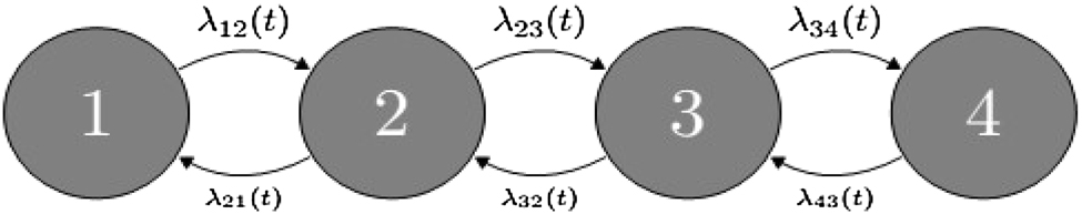
Estimation of the transition matrix of the semi-Markov Process

The transition matrix Λ _ij includes four exclusive states and six transitions, and the elements of this matrix are the hazard functions λ _ij for each possible transition. Note that for the current study three main functions of transitions (hazard rates) were selected: λ 12 z , λ 23 z , and λ 34 z .

Whereas the functions λ 21 z , λ 32 z and λ 43 z represent the instantaneous risks of death, for the child of the order i, (respectively) i: 1, 2, 3. We can draw the transition diagram for this transition matrix as:

For the application purpose, the R package: “SemiMarkov” was used, and the command “hazard” under “semimarkov” function returns the estimates of the hazard rates λ i j z related with all sojourn times.

Effects of covariates on Sojourn times

Generally, the main objective behind the construction of semi-Markov models is to estimate the effects of the individual characteristics x i j t on the rate (risk) function λ i j z (or other functions) for all possible transitions between states i and j. Mathematically, the way we introduce these covariates in our models is based on proportionality assumptions developed in survival analysis (Cox 1972, 1975) and (Andersen 1988, 1993). We define x i j ̲ , a vector of all covariates related to the transition i → j, and we note λ i j 0 z the baseline risk function for this transition, therefore, each possible transition of SMP can take different λ i j 0 z baseline functions. After including x i j ̲ , the total risk function is given as:

Where: ψ x i j ̲ is a functional form of the covariables, usually, we select an exponential form: ψ x i j ̲ = exp β i j t x i j , as in proportional hazard model (Cox 1972). The likelihood method was used for estimation, and for more flexibility and accuracy, different probability distributions of the sojourn times were adjusted for each transition i → j. As another indication, the SemiMarkov R package that we used in the application provides three distributions for the sojourn time data: the Exponential, Weibull, and Exponentiated-Weibull. Finally, when estimating the semi-Markov models, we followed the approach of the intensity transition functions as in proportional hazard models.

Before proceeding to the analysis of the results, we put hereafter notations and definitions relative to the semi-Markov models projected on the studied phenomenon.

1. The states of the process i, j: 0, 1, …, k: are the children ever born for women;

2. Transitions (i → j) and (j → i) are recorded if there is a newborn or death of a child;

3. The date of transition t _i,j : is the date of birth or death of the child, (the methodology of the MICS4 survey record: day, month and year of birth or dead);

4. The sojourn time (birth interval) s _i,j in the state i before switch to the state j: is the difference between the date of birth of the child of the rank i and the date of birth of the child of rank i + 1 or the date of death of that child. Except for the first child s _i,j equals the difference between the birth date of the first child and the date of marriage.

5. Of course, and after birth, there are about 9 months, where the mother cannot give birth again; (which is considered when we estimate the different birth intervals);

6. Transitions of type i → i, are considered as right-censored.

7. On the last note, we excluded the twins and triples pregnancies from analysis, as a result, the hazard rate functions λ 13 z , λ 14 z , λ 24 z are not considered in the transition matrix.

Data description of the MICS4 of Algeria

In Algeria, the MICS4 survey targeted a sample of 28,000 households. It provides representative statistics of the Algerian population at the national level and at the level of its territories. Its purpose is to highlight the progress made towards the Millennium Development Goals as well as the national development goals, and in particular, those relatives of the well-being of families, children, and women. The MICS4 Algeria survey was conducted from mid-2012 to the end of 2013 by the Ministry of Health, Population, and Hospital Reform (MSPRH) with technical and financial support from UNICEF, and as well as financial contribution of the United Nations Population Fund (UNFPA). We noted that Algeria conducted three editions of MICS surveys: MICS1 in 1995, MICS2 in 2000, MICS3 in 2006, and MICS4 in 2012.

Regarding the modeling purposes, we resume here the inclusion criteria are as follows: For the birth intervals taking account are the 4th, 5th, and 6th children. The unit measure of the birth interval was months. We have 13,453 as the total number of children in the database for fourth, fifth, and sixth birth orders. Finally, we excluded twin and triplet pregnancies from the analysis.

Estimation results

As the three distributions of the sojourn times are nested, which is discussed in Section 2.2, we followed this strategy to select the optimal distribution by using the Wald tests, firstly, we start by fitting the Exponentiated–Weibull E W η i j , ϑ i j , θ i j , for all possible transitions if θ _ij = 1, we fit the Weibull distributions W η i j , ϑ i j , and if ϑ _ij = 1, we fit the Exponential distribution. Note that for all transitions, the optimal model is the Weibull distribution, as shown in Table 1, and the results of the Exponentiated–Weibull distribution are reported in Table 5 in the Appendices.

Recalling that the objective of this application is to analyze the birth intervals of the 4th, 5th, and 6th child. Thus, by estimating of the semi-Markov models, we focused on studying transitions 3 → 4, 4 → 5, and 5 →6. For the transition matrix of the semi-Markov process (Section 2.3), the estimated results are summarized in the following matrix. On the other hand, the transition graph contains the hazard functions λ _ij and not the transition probabilities p _ij .

The risk of transition from state 3 to state 4 is λ ₃₄(t) = 0.0016, which indicates (all other things being equal) that each month past the risk (chance) that a woman gives birth to the 4th child is 0.0016. The same hazard rate for transitions 4 → 5 and 5 → 6, with average rates of λ ₄₅(t) = 0.001 and λ 56 t = 0.001 5 ; the full results are presented in Table 4 in the Appendix. Under this finding, and with a slight difference, we can accept the assumption that the transition rate from the third to the fourth birth is identical (homogeneous) to the transition rate from the fourth to the fifth birth and from the fifth to the sixth birth. In practice, the hypothesis of homogeneity in transition rates depends on different factors (population, cultural context, birth orders, etc.); for example, this hypothesis was rejected by (Hotz, Heckman, and Walker 1985) for the first, second, and third births.

On the other hand, functions λ 43 t = 0.000 2 , λ 54 t = 0.000 3 and λ 65 z = 0.001 represent the instantaneous risks of mortality for the ith child where: i: 4, 5, 6. We can explain that infants born fourth and fifth have nearly the same mortality risk; in contrast, infants born sixth have a higher risk of death than fifth and fourth-born. The study conducted by (Chellai and Boudrissa 2019) is a well-designed research on this topic.

Model adequacy

The Akaike information criterion (AIC) and logarithm of the likelihood function were used to analyze the adequacy and goodness of fit of the semi-Markov model. When estimating a statistical model, it is possible to increase the likelihood of the model by adding a parameter. The Akaike information criterion, such as the Bayesian information criterion, makes it possible to penalize the models according to the number of parameters to satisfy the criterion of parsimony.

For model validation, we chose the model with the smallest Akaike information criterion (AIC) values. In practice, the AIC criterion deals with the under-fitting and over-fitting problems simultaneously. Among the competitive models, the optimal model was model 2, which included all covariates and took a Weibull distribution as a sojourn time function for the three transitions of interest in this study (3–4, 4–5, and 5–6), see Table 1. Furthermore, model (2) is the most parsimonious with a log-likelihood function equal to −18,681.21, and an AIC criterion of 37,404.42.

Is there a difference in birth intervals between household living areas?

In Algeria, fertility dynamics based on the area of residence showed that the decline in fertility rates was more accentuated in urban areas than in rural areas. For example, we recorded 5.3 children per woman in the 1970s, and this rate reached 2.6 children per woman in 2013 in urban areas compared to 7.2 and 2.9 children per woman in rural areas. Over this period (1970–2012), the Algerian population experienced the first, second, and third stages of the demographic transition (Kirk 1996).

The estimated results in Table 2 showed that the coefficients of the area of residence are statistically insignificant (at the significance level α = 0.05); despite that, we can practically accept the two estimated parameters of the 5th and 6th child with a level of significance α = 0.1 and α = 0.15 (respectively). Thus, we can report that mothers in urban areas have 6.4 and 7.4% less risk of giving birth to the 5th and 6th child compared to mothers in rural areas. In other words, mothers in urban areas have long birth intervals for the 5th and 6th child compared to mothers in rural areas, as shown by the hazard functions in Figure 1.

Figure 1:

Semi-Markov process hazard rate function according to area of residence.

Source: MICS4 database of Algeria. (a): For the 4th child (b): for the 5th child and (c) for the 6th child.

In another context, we think that some non-adjusting factors, such as contraceptive use and infant mortality, could confound the main effect on the length of the birth intervals. However, with globalization and the tendency to construct a standard family (just with two or three children) by parents, it can be concluded that the zone classification as rural vs. urban becomes a critical discriminating factor in almost all demographic studies. In addition, and far from the complexity of classifying the geographical areas by rural and urban areas as reported by (Pateman 2011), we think that the difference in birth intervals between women in urban and rural areas was confused by several factors such as the mothers’ education levels, wealth index, and previous birth intervals, as depicted for the 4th child in Figure 1 bloc (a).

When we see the total fertility rates in the Algerian population (Figure 2), the distribution by area of residence showed that the rural area has the highest TFR compared to the urban area, and this is for all the age categories of the mother. As an indication, the TFR was 148 (births per 1,000 women) for women living in rural areas and aged 25–39 years which represents the highest value of the TFR index.

Figure 2:

Total fertility rate (TFR) by age group and area of residence in Algeria.

Source: edited from the final report of the MICS4 survey (MSPRH 2015), p. 127.

Family income and birth spacing

We note that an explicit variable that measures the level of a household’s income is not available in the database of the MICS4 of Algeria, and given the importance of this factor to analyze the birth spacing, as an alternative (or a proxy variable), we use the wealth index, which is calculated for each household using Principal Component Analysis (PCA) (Jolliffe 2011). Several variables were included to estimate this index, such as information about the ownership of consumer goods, house characteristics, water, and sanitation, among others; more details on how to estimate the wealth index can be found in the study conducted by (Shea et al. 2004).

Through the estimate results in Table 3, the wealth index sign is well adequate with the demographic literature in this field, see Kamal and Pervaiz (2012), additionally, the three estimate coefficients are statistically significant, we can report this result as: if the wealth index increase by one unit, the risk to delivering the 4th, 5th and 6th child should be decreased (ceteris paribus) by 7, 7.3, and 11.9%, and the effect of such variable is more clear for sixth birth interval compared to fifth and fourth birth intervals. Overall, this implies that women living in wealthy families have wider birth intervals.

Do less educated mothers have long birth intervals?

Regarding the educational level of mothers, the estimated results in Table 2 show that the higher the mother’s education level, the higher the risk (or chance) of having the 4th, 5th and the 6th child. We used illiterate mothers as a reference group, and the corresponding regression coefficients were statistically significant for the three children and all mothers’ education levels, except the primary level for the fourth child. In terms of the relative risks, mothers with primary education level have 20 and 36.7% lower risks (respectively for the 5th and 6th child) to have a new child compared to the illiterate mothers; in contrast, in terms of birth intervals, they are likely to have longer intervals compared to illiterate mothers. Figure 3 illustrates the hazard rate functions of the Semi-Markov Process, and from the 4th child to the 6th child, the common feature of all mothers is that they showed a decreasing risk trend to deliver a new child, we see clearly that across the maximum values of the hazard functions in Figure 3, e.g. for the 4th child the maximum value is 0.04, for the 5th child is 0.02 and for the 6th child is 0.015.

Figure 3:

The hazard functions of the semi-Markov by the mothers’ education levels for the three transitions: (a) for the 4th child, (b) for the 5th child, and (c) for the 6th child.

Source: Plotting using “SemiMarkov” package. Numbers beside and under plots in each figure are (1) illiterate, (2) primary (3) middle (4) secondary and (5) high educational level.

Mothers with middle educational level have 13, 40, and 61% lower risk of giving birth to a new child, respectively, to the 4th, 5th, and 6th children compared to the illiterate mothers; however, in terms of birth intervals, they are likely to have longer intervals compared to illiterate mothers. The mothers belonging to the secondary education level had, respectively, the 4th, 5th, and 6th child 15.3, 49.4, and 71.7% lower risks of giving birth to a new child compared to illiterate mothers. However, in terms of birth intervals, they are likely to have longer intervals compared to illiterate mothers. The most significant pattern is for the mothers who achieved a high education level; they have, respectively, for the 4th, 5th, and 6th children 72.6, 40, and 87.1% lower risks of giving birth to a new child compared to the illiterate mothers; however, in terms of birth intervals, they are likely to have longer intervals compared to illiterate mothers. This pattern is confirmed when we place the number of children vs. the mothers’ education levels, we found that mothers who were illiterate or primarily educated had the highest number of children, which means high fertility rates.

However, there is an interaction between the educational level of women and the age at first marriage; this interaction could, in turn, affect the distribution of births in women of reproductive age (Ouadah-Bedidi 2005). The mechanism of this interaction has been reported by (Hotz, Heckman, and Walker 1985). In addition to this trend of less-educated women (illiterate or primary level) to build large families, the same women recorded the highest rates of child mortality compared to higher-level education, which was confirmed in the final report of the MICS4 survey, which showed that there were 26 deaths per 1,000 live births from illiterate mothers compared to 19 deaths per 1,000 live births from mothers with secondary or high educational levels (MSPRH 2015).

Does the previous birth interval affect the current birth interval?

The previous birth interval measures the length of time s _i,j between the date of birth of the jth and ith child, and was included in the model to test the hypothesis of homogeneity of the birth intervals. At the same point (Khalifa 1989) considered previous birth intervals as a measure of couple-specific behavior and fecundability. Otherwise, we tried to estimate the effect of this duration s _i,j on the future birth interval s _j,j+1, (e.g., the effect of the 3rd childbirth interval on the 4th childbirth interval, etc.). The estimated results (summarized in Table 2) show that all regression coefficients are statistically significant, with a small effect of the previous birth intervals on the current intervals. Consequently, we can report the estimated results as follows: if the 3rd birth interval increased by (in months), the birth interval the for 4th child was 7% likely to decrease, and if the 4th birth interval increased (in months) the birth interval of the 5th child was 7.3% likely to decrease, and if the 5th birth interval increased (in months) the birth interval of the 6th child was 10% likely to decrease. This result is relatively similar to that reported by (Rodriguez et al. 1984). As a broad note for this variable, we presume that the weakness of the relationship between the previous and current birth intervals could be generated by a combination of biological and behavioral factors; however, these factors cannot be controlled using the methodology of this study, as well as through the statistical data currently available.

References

Abdel-Fattah, M., T. Hifnawy, T. I. El Said, M. M. Moharam, and M. A. Mahmoud. 2007. “Determinants of Birth Spacing Among Saudi Women.” Journal of Family and Community Medicine 14 (3): 103.10.4103/2230-8229.97098Search in Google Scholar
Ahmad, I., and Y. R. Dewi. 2020. “Birth Intervals and Infant Mortality in Indonesia.” Population Review 59 (1): 73–84. https://doi.org/10.1353/prv.2020.0003.Search in Google Scholar
Altınok, Y., and D. Kolçak. 1999. “An Application of the Semi-Markov Model for Earthquake Occurrences in North Anatolia, Turkey.” Journal of the Balkan Geophysical Society 2: 90–9.Search in Google Scholar
Andersen, P. K., O. Borgan, R. D. Gill, and N. Keiding. 1993. Statistical Models Based on Counting Processes. New York: Springer-Verlag.10.1007/978-1-4612-4348-9Search in Google Scholar
Andersen, P. K. 1988. “Multistate Models in Survival Analysis: A Study of Nephropathy and Mortality in Diabetes.” Statistics in Medicine 7 (6): 661–70. https://doi.org/10.1002/sim.4780070605.Search in Google Scholar PubMed
Baschieri, A., and A. Hinde. 2007. “The Proximate Determinants of Fertility and Birth Intervals in Egypt: An Application of Calendar Data.” Demographic Research 16: 59–96. https://doi.org/10.4054/demres.2007.16.3.Search in Google Scholar
Benojir, A., Md. Rasel Kabir, Md. Menhazul Abedin, A. Mohammad, and Md. Akhtarul Islam. 2019. “Determinants of Different Birth Intervals of Ever Married Women: Evidence from Bangladesh.” Clinical Epidemiology and Global Health 7 (3): 450–6.10.1016/j.cegh.2019.01.011Search in Google Scholar
Blasi, A., J. Janssen, and R. Manca. 2004. Numerical Treatment of Homogeneous and Non-homogeneous Semi-Markov Reliability Models, pp. 697–714.10.1081/STA-120028692Search in Google Scholar
Chang, S. H., and S. J. Tzeng. 2006. “Nonparametric Estimation of Sojourn Time Distributions for Truncated Serial Event Data—A Weight-Adjusted Approach.” Lifetime Data Analysis 12 (1): 53–67. https://doi.org/10.1007/s10985-005-7220-9.Search in Google Scholar PubMed
Chellai, F., and N. Boudrissa. 2019. “Excess Infant Mortality of Twins over Singletons in Arab Countries: The Evidence of Relative Survival Methods.” Twin Research and Human Genetics 22 (4): 255–64. https://doi.org/10.1017/thg.2019.30.Search in Google Scholar PubMed
Choo, S. 2020. Semi-Markov Toolbox MATLAB Central File Exchange. Also available at https://www.mathworks.com/matlabcentral/fileexchange/49980-semi-Markov-toolbox.Search in Google Scholar
Conde-Agudelo, A., A. Rosas‐Bermudez, F. Castaño, and M. H. Norton. 2012. “Effects of Birth Spacing on Maternal, Perinatal, Infant, and Child Health: A Systematic Review of Causal Mechanisms.” Studies in Family Planning 43 (2): 93–114.10.1111/j.1728-4465.2012.00308.xSearch in Google Scholar PubMed
Cox, D. R. 1972. “Regression Models and Life Tables.” Journal of the Royal Statistical Society: Series B 34: 187–220. https://doi.org/10.1111/j.2517-6161.1972.tb00899.x.Search in Google Scholar
Cox, D. R. 1975. “Partial Likelihood.” Biometrika 62 (2): 269–76. https://doi.org/10.1093/biomet/62.2.269.Search in Google Scholar
D’Amico, G., J. Janssen, and R. Manca. 2006. “Homogeneous Semi-Markov Reliability Models for Credit Risk Management.” Decisions in Economics and Finance 28 (2): 79–93.10.1007/s10203-005-0055-8Search in Google Scholar
Fallahzadeh, H., Z. Farajpour, and Z. Emam. 2013. “Duration and Determinants of Birth Interval in Yazd, Iran: A Population Study.” Iranian Journal of Reproductive Medicine 11 (5): 379.Search in Google Scholar
Foucher, Y., E. Mathieu, P. Saint-Pierre, J. F. Durand, and J. P. Daures. 2005. “A Semi-Markov Model Based on Generalized Weibull Distribution with an Illustration for HIV Disease.” Biometrical Journal 47 (6): 825–33. https://doi.org/10.1002/bimj.200410170.Search in Google Scholar PubMed
Ganatra, B., and A. Faundes. 2016. “Role of Birth Spacing, Family Planning Services, Safe Abortion Services and Post-abortion Care in Reducing Maternal Mortality.” Best Practice & Research Clinical Obstetrics & Gynaecology 36: 145–55. https://doi.org/10.1016/j.bpobgyn.2016.07.008.Search in Google Scholar PubMed
Ginsberg, R. B. 1972. “Critique of Probabilistic Models: Application of the Semi‐Markov Model to Migration.” Journal of Mathematical Sociology 2 (1): 63–82. https://doi.org/10.1080/0022250x.1972.9989803.Search in Google Scholar
Hoem, J. M. 1972. “Inhomogeneous Semi-Markov Processes, Select Actuarial Tables, and Duration-Dependence in Demography.” In Population Dynamics, 251–96. Madison: Academic Pressbook-chapter.10.1016/B978-1-4832-2868-6.50013-8Search in Google Scholar
Hotz, V. J., J. J. Heckman, and J. Walker. 1985. “New Evidence on the Timing and Spacing of Births.” American Economic Review 75 (2): 179–84.Search in Google Scholar
Jolliffe, I. 2011. “Principal Component Analysis.” In International Encyclopedia of Statistical Science, edited by M Lovric. Berlin: Springerbook-chapter.10.1007/978-3-642-04898-2_455Search in Google Scholar
Kamal, A., and M. K. Pervaiz. 2012. “Determinants of Higher Order Birth Intervals in Pakistan.” Journal of Statistics 19: 54–82.Search in Google Scholar
Khalifa, M. 1989. “Determinants of Birth Intervals in Sudan.” Journal of Biosocial Science 21 (3): 301–20. https://doi.org/10.1017/s0021932000018009.Search in Google Scholar PubMed
Kirk, D. 1996. “Demographic Transition Theory.” Population Studies 50 (3): 361–87. https://doi.org/10.1080/0032472031000149536.Search in Google Scholar PubMed
Koenig, M. A., J. F. Phillips, O. M. Campbell, and S. D’Souza. 1990. “Birth Intervals and Childhood Mortality in Rural Bangladesh.” Demography 27 (2): 251–65. https://doi.org/10.2307/2061452.Search in Google Scholar
Kouaouci, A. 1993. “Essai de reconstitution de la pratique contraceptive en Algérie durant la période 1967–1987.” Population 48 (4): 859–83.10.2307/1533880Search in Google Scholar
Król, A., and P. Saint-Pierre. 2015. “SemiMarkov: An R Package for Parametric Estimation in Multi-State Semi-Markov Models.” Journal of Statistical Software 66 (6): 1–16.10.18637/jss.v066.i06Search in Google Scholar
Lessard, S. 2014. Processus Stochastiques: Cours et exercices Corriges. Paris: Editions ellipses.Search in Google Scholar
Limnios, N., and G. Oprisan. 2012. Semi-Markov Processes and Reliability. Boston: Springer Science Business Media.Search in Google Scholar
McKinney, D., M. House, A. Chen, L. Muglia, and E. DeFranco 2017. “The Influence of Interpregnancy Interval on Infant Mortality.” American Journal of Obstetrics and Gynecology 216 (3): 316.e1–e9. https://doi.org/10.1016/j.ajog.2016.12.018.Search in Google Scholar PubMed PubMed Central
Miller, J. E. 1991. “Birth Intervals and Prenatal Health: An Investigation of Three Hypotheses.” Family Planning Perspectives: 62–70. https://doi.org/10.2307/2135451.Search in Google Scholar
Mitchell, C. E., M. G. Hudgens, C. C. King, S. Cu‐Uvin, Y. Lo, A. Rompalo, and J. S. Smith. 2011. “Discrete‐time Semi‐Markov Modeling of Human Papillomavirus Persistence.” Statistics in Medicine 30 (17): 2160–70. https://doi.org/10.1002/sim.4257.Search in Google Scholar PubMed PubMed Central
MSPRH 2015. Rapport finale de l’Enquête par grappes a indicateurs multiples (MICS4), Unicef FNUP, MSPRH (Algerie). Also available at https://www.unicef.org/algeria/sites/unicef.org.algeria/files/2018-04/Rapport%20MICS4%20%282012-2013%29.pdf.Search in Google Scholar
Mudholkar, G. S., and D. K. Srivastava. 1993. “Exponentiated Weibull Family for Analyzing Bathtub Failure- Rate Data.” IEEE Transactions on Reliability 42 (2): 299–302. https://doi.org/10.1109/24.229504.Search in Google Scholar
Nair, S. 1996. “Determinants of Birth Intervals in Kerala: An Application of Cox’s Hazard Model.” Genus 52 (3/4): 47–65.Search in Google Scholar
Négadi, G., D. Tabutin, and J. Vallin. 1974. “Situation démographique de l’Algérie.” In La Population de L’Algérie, 16–62. Paris: CICRED.Search in Google Scholar
Négadi, G., and J. Vallin. 1974. “La fécondité des algériennes : niveaux et tendances.” Population 29 (3): 491–515.10.2307/1530917Search in Google Scholar
Ouadah-Bedidi, Z. 2005. “Baisse de la Fécondité en Algérie : Transition de Développement ou Transition de Crise.” In Thèse en Sciences économiques. Démographie économique. Paris: Institut d’études politiques.Search in Google Scholar
Ouadah-Bedidi, Z., and J. Vallin. 2013. “Fertility and Population Policy in Algeria: Discrepancies between Planning and Outcomes.” Population and Development Review 38: 179–96. https://doi.org/10.1111/j.1728-4457.2013.00559.x.Search in Google Scholar
Paes, A., and A. Lima. 2004. “A SAS Macro for Estimating Transition Probabilities in Semiparametric Models for Recurrent Events.” Computer Methods and Programs in Biomedicine 75: 59–65. https://doi.org/10.1016/j.cmpb.2003.08.007.Search in Google Scholar PubMed
Palloni, A., and S. Millman. 1986. “Effects of Inter-birth Intervals and Breastfeeding on Infant and Early Childhood Mortality.” Population Studies 40 (2): 215–36. https://doi.org/10.1080/0032472031000142036.Search in Google Scholar
Pateman, T. 2011. “Rural and Urban Areas: Comparing Lives Using Rural/urban Classifications.” Regional Trends 43: 11–86. https://doi.org/10.1057/rt.2011.2.Search in Google Scholar
Perman, M., A. Senegacnik, and M. Tuma. 1997. “Semi-Markov Models with an Application to Power-Plant Reliability Analysis.” IEEE Transactions on Reliability 46 (4): 526–32. https://doi.org/10.1109/24.693787.Search in Google Scholar
Rabbi, A. M. F., S. C. Karmaker, S. A. Mallick, and S. Sharmin. 2013. “Determinants of Birth Spacing and Effect of Birth Spacing on Fertility in Bangladesh.” Dhaka University Journal of Science 61 (1): 105–10. https://doi.org/10.3329/dujs.v61i1.15105.Search in Google Scholar
Rodriguez, G., J. Hobcraft, J. McDonald, J. Menken, and J. Trussell. 1984. “A Comparative Analysis of Determinants of Birth Intervals.” In WFS Comparative Studies: Cross-National Summaries (World Fertility Surveys). Voorburg, Netherlands: International Statistical Institutebook-chapter.Search in Google Scholar
Shea, O. R., and J. Kiersten. 2004. “The Dhs Wealth Index”. Technical Report, Calver- Ton, Maryland : ORC Macro.” In DHS Comparative Reports No. 6.Search in Google Scholar
Solaiman, B. 2006. Processus Stochastiques Pour L’ingenieur. Lausanne: Presses Polytechniques et universitaires romandes.Search in Google Scholar
Suwal, J. V. 2001. “Socio-cultural Dynamics of Birth Intervals in Nepal.” Contributions to Nepalese Studies 1: 11–33.Search in Google Scholar
UNICEF 2020. Multiple Indicator Cluster Survey (MICS). Also available at http://mics.unicef.org/surveys.Search in Google Scholar
Wanneveich, M., Helene Jacqmin-Gadda, J.-F. Dartigues, and P. Joly. 2018. “Projections of Health Indicators for Chronic Disease under a Semi-Markov Assumption.” Theoretical Population Biology 119: 83–90. https://doi.org/10.1016/j.tpb.2017.11.006.Search in Google Scholar PubMed
Weibull, W. 1951. “A Statistical Distribution Function of Wide Applicability.” Journal of Applied Mechanics 18: 292–7. https://doi.org/10.1115/1.4010337.Search in Google Scholar
Weijing, W. 2003. “Nonparametric Estimation of the Sojourn Time Distributions for a Multipath Model.” Journal of the Royal Statistical Society Series B (Statistical Methodology) 65: 921–35.10.1046/j.1369-7412.2003.00423.xSearch in Google Scholar
Wu, B., L. Cui, and C. Fang. 2019. “Reliability analysis of semi-Markov systems with restriction on transition times.” Reliability Engineering & System Safety 190: 1–10. https://doi.org/10.1016/j.ress.2019.106516.Search in Google Scholar
Supplementary Material
The online version of this article offers supplementary material (https://doi.org/10.1515/em-2021-0030).
© 2021 Walter de Gruyter GmbH, Berlin/Boston
Articles in the same Issue
- Research Articles