Equations involving the modular 𝑗-function and its derivatives
-
Vahagn Aslanyan

 ,
Sebastian Eterović
and
Vincenzo Mantova
,
Sebastian Eterović
and
Vincenzo Mantova

Abstract
We show that, for any polynomial
1 Introduction
The problem of determining which (systems of) equations involving certain classical transcendental functions of a complex variable have solutions is a natural question at the intersection between complex geometry, model theory, and number theory. In complex geometry, it is a form of analytic Nullstellensatz for the given functions; in model theory, it plays an important role in the definability properties of the functions involved; and in number theory, it is related to Schanuel’s conjecture and its analogues (given by special cases of the Grothendieck–André generalised period conjecture). Often, the function under consideration is of arithmetic importance. Examples of such classical functions are the exponential functions of semi-abelian varieties and Fuchsian automorphic functions. In this paper, we focus on the modular 𝑗-function and its derivatives.
The first conjecture in this area arose from Zilber’s work on the model theory of complex exponentiation [17, 16, 18].
It is now referred to as the Exponential (Algebraic) Closedness conjecture or Zilber’s Nullstellensatz, and predicts when systems of equations involving addition, multiplication, and complex exponentiation have solutions in the complex numbers.
We refer to the general version of the problem as Existential Closedness, or EC for short.
An EC conjecture for the 𝑗-function was proposed in [4, §1]; in geometric terms, it states that any algebraic variety
If one somehow knows that an algebraic variety 𝑉 does intersect the graph of 𝑗, a very natural next question is to determine how these intersection points are distributed within 𝑉.
For instance, one may ask whether these points are Zariski dense in 𝑉.
We remark that if
In the same work [4], the authors also proposed an extension of the conjecture incorporating the derivatives of 𝑗 (see [4, Conjecture 1.6]).
This version of EC is often referred to as Existential Closedness with Derivatives, or ECD for short.
This time the variety 𝑉 in question is a subset of
Very few cases of ECD have been proven, in comparison to EC where various families of varieties in
In this article, we prove the ECD conjecture when
Our first main result establishes the existence of solutions in all non-trivial cases.
Let
has infinitely many solutions.
The proof of Theorem 1.1 is based on a generalisation of the methods of [9], which use Rouché’s theorem from classical complex analysis to establish some cases of EC for 𝑗 (without derivatives).
Theorem 1.1 can be seen as an analogue of the classical fact that every irreducible polynomial
Throughout the paper, all algebraic subvarieties of
Our main goal is to obtain a much stronger version of Theorem 1.1.
We show that, for any polynomial
is Zariski dense in the hypersurface
We remind the reader that this is equivalent to establishing certain cases of ECD for subvarieties of
The bulk of the paper is focused on proving the Zariski density of the set of solutions, which the proof of Theorem 1.1 does not provide. For instance, the solutions of the equation
found via the proof Theorem 1.1 are the
The zeroes of
This immediately gives that the three equations
For any polynomial
is Zariski dense in the hypersurface
For every rational function
where 𝐻 is a polynomial and
A special case of Theorem 1.2 is that the equation
In [8], the author studies the problem of finding generic solutions to equations involving 𝑗 (and its derivatives) under the assumption that the system has a Zariski dense set of solutions.
In particular, combining Theorem 1.2 with [8, Theorem 6.5], we get that there is a countable field
To prove Theorem 1.2, we establish general criteria for the solvability of certain equations involving periodic functions (see Section 4). The following proposition is a special case of those criteria.
A meromorphic function
Let
there is
Let us consider an example illustrating how we apply Proposition 1.6 in practice. It also gives an idea of our approach in the general case.
Consider the equation
where either
Thus we obtain an equation in a suitable form for using Proposition 1.6, where
has a pole at
has no finite poles, but it has limit ∞ as
Thus, by Proposition 1.6, there is a sequence
To deduce Zariski density of these solutions, suppose that all of them are also solutions of another independent equation
We also note that our criteria can be applied to more general periodic functions, beyond polynomials of
1.1 Structure of the paper
In Section 2, we go over some basic preliminaries about the 𝑗-function and its derivatives.
We also give the definition of Zariski density used in Theorem 1.2.
In Section 3, we prove Theorem 1.1 by extending the methods of [9], which are based on Rouché’s theorem.
In Section 4, we prove criteria for the existence and distribution of solutions of equations involving periodic functions, which combined imply Proposition 1.6 (but are significantly more general). The approach used here involves Rouché’s theorem, the Argument Principle, and some elementary methods from valuation theory.
These methods do not appear in later sections of the paper.
In Section 5, we use the results of the previous section to obtain concrete criteria for proving Zariski density of equations of the form
2 Preliminaries
Let ℍ denote the complex upper half-plane
This action can be seen as a restriction of the action of
As a group,
The modular 𝑗-function can be defined as the unique
In fact,
Since 𝑗 is invariant under the action of
We let
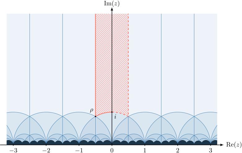
The fundamental domains of the action by
It is well known that 𝑗 satisfies the following third-order differential equation (and none of lower order [15]):[2]
This shows that the derivatives of 𝑗 of order at least 3 are rational over 𝑗,
The functions 𝑗,
Observe that
Using (2.1) and the 𝑞-expansions of
We finish this section with the definition of what we mean by finding a Zariski dense set of solutions to an equation.
Let
has a Zariski dense set of solutions if, for any polynomial
Clearly, it suffices to prove Zariski density for irreducible polynomials to obtain Theorem 1.2, so from now on, we will reduce to the case where 𝐹 is irreducible.
3 Existence of solutions
We start with the Rouché method for proving the existence of solutions, but not yet their Zariski density. We first recall the crucial theorem.
Theorem 3.1 (Rouché; see e.g. [14, Chapter VI, §1, Theorem 1.6])
Let
holds for all 𝑧 on 𝐶, then the difference between the numbers of zeroes and poles in the interior of 𝐶 for the functions
It is well known that the Euclidean closure of the
Let
If
If
Proof
(i) We first show that
Conversely, assume now that
Thus we may assume
Therefore,
This implies
On the other hand,
Since
we see that
(ii) As
In order to ease notation, we will start using bold-faced letters to denote vectors, so we set
We are now ready to prove Theorem 1.1 which we restate below for convenience.
For every
Proof
If 𝐹 does not depend on
Let
Then we want to solve the equation
Notice that
Pick a point
We have
Consider the polynomial
We can now shrink 𝐵 to make sure that
and we can apply Rouché’s theorem to these functions.
Since 𝑓 has a zero in
The following more general statement can be proven by the same argument.
Let
As mentioned in Section 1, the proof of Theorem 1.1 does not guarantee a Zariski dense set of solutions.
For instance, if
4 Solvability of certain equations involving periodic functions
In this section, we establish some general criteria for the solvability of equations involving periodic functions and, in particular, prove Proposition 1.6. We remark that this section is independent in many ways from the rest of the paper as the results we prove make no reference to 𝑗 or its derivatives, and in particular, the methods developed here will not reappear in the following sections.
We recall that, given a meromorphic function 𝑓, not identically 0, and a point
Let
If
has ℓ solutions, counted with multiplicity, in
Proof
For simplicity, assume that
Under the above assumptions,
Pick a small closed disc 𝐷 centred at
By Rouché’s Theorem 3.1, the number of zeroes of the functions
inside 𝐷 is the same.
Since the former has a zero at
Finally, note that
This finishes the proof of the proposition when
Following the notation of the proposition, when the
As the following example shows, we may also need to consider non-periodic functions which are asymptotically periodic. Dealing with those functions requires a considerably more sophisticated setup than the one in Proposition 1.6, so we first discuss the example in detail to clarify the choices made in the rest of this section.
Consider the equation
where 𝛼 is to be determined later.
In order to write this equation as a polynomial in 𝑧 with periodic coefficients, we apply the
In this example, the ratio of the coefficients of
In this particular example, the ratio in question is between the coefficients of
We claim that
and because of the extra factor
This fact is responsible for the technicalities in the rest of this section.
It is worth mentioning that, for equations of the form
The reader may benefit from revisiting this example after reading the rest of the paper, as it will make the above-mentioned phenomena less obscure.
Let 𝒫 denote the field of 1-periodic meromorphic functions on ℍ which are also meromorphic at
Also, given an unbounded region
Let
Proof
It suffices to prove the conclusion for
Each
It now suffices to specialise at
It follows at once that all functions in
Call the order at
in the region
We say that 𝑓 has exponential growth at
Here we consider
We can now set up a generalisation of Proposition 4.1 that will cover our application to 𝑗. Let us fix the following data:
a polynomial
a value 𝑠 which is either 0 or 1.
We look for the zeroes of functions of the form
We first parametrise the roots of
There is a positive
there are holomorphic functions
Moreover, there are
Proof
It suffices to prove the conclusion for 𝐹 irreducible as a polynomial over
Let
Now fix some 𝑘.
For every
and since
Let
By Lemma 4.3 combined with the above inequalities, there is
for some fixed determination of
Let 𝑆 be the set of indices 𝑡 such that
where now
is bounded and continuous, it must converge to a non-zero root
We now provide an estimate on the size of
There exist
for all
Proof
We work in a region
By Lemma 4.5, provided
parametrising the roots of
Since we are assuming
It follows, for instance, that
We now bound
If
This ensures that
Suppose that
If
We first give bounds when
For
Now choose
Now, if
for any
We now recall the Argument Principle, which plays a key role in the proof of Proposition 4.8.
Theorem 4.7 (Argument Principle; see e.g. [14, Chapter VI, §1, Theorem 1.5])
Let 𝑓 be a meromorphic function on a complex domain Ω. Let 𝐶 be a simple closed curve (positively oriented) which is homologous to 0 in Ω and such that 𝑓 has no zeroes or poles on 𝐶. Let 𝑍 and 𝑃 respectively denote the number of zeroes and poles (counted with multiplicity) of 𝑓 in the interior of 𝐶. Then
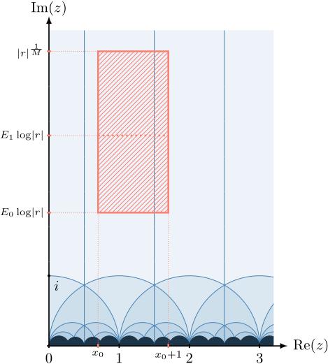
The region
In the proof of the following proposition, we will integrate
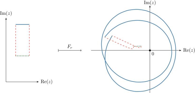
Visual representation of the action of
Let
where
Proof
Recall that
for
Note that
Vertical sides. We show that the images of the vertical sides of
First, we observe that
Since
Likewise,
for
Bottom side. We now show that the image of the bottom side is away from 0 and cannot wind much. Using (4.1), for 𝑟 sufficiently large,
Top side. We show that
We now constraint 𝑤 to the region
By construction,
In particular, by Lemma 4.6, we find that
Therefore, we find that there is
Observe that, for 𝑟 large enough, we have
Thus, for sufficiently large 𝑟, we have
Conclusion. Using the above estimates, we can now find the winding number of
By the Argument Principle, the integral on the left-hand side must be the difference between the number of zeroes and poles of
Proof of Proposition 1.6
This follows from combining Propositions 4.1 and 4.8, where we use
5 Some criteria for Zariski density
Recall that
5.1 Generic transforms
Given
In particular, we have
Note that
We make the following observations.
The map
For each
For any
Indeed, let
Thus
Since
For any
Indeed, note that if 𝑝 is not a unit (meaning it contains one of the variables
Let 𝑝 be an irreducible polynomial in
Proof
By 3 and 4,
5.2 Density criteria
We now apply the results of Section 4 to establish some useful criteria for Zariski density of solutions of equations involving
Given a function
Let
Proof
Fix some
Likewise, set
If 𝛾 is upper triangular, namely
Otherwise, let
Thus, as soon as 𝑧 is sufficiently large, the last factor on the right-hand side has modulus less than
Therefore, by Rouché’s Theorem 3.1,
Let
Proof
Suppose by contradiction that all the solutions of
By Propositions 4.1 and 5.3, for
Let
Proof
If
6 Zero estimates
In view of the results in the previous section, we will now look at the poles of quotients of the form
Given
For every
Proof
Immediate. ∎
First, we consider unramified points of 𝑗, that is, points
Let
Proof
Let
From now on, we assume
Now take
where
The map
by the fibre-dimension theorem, 𝜐 is also dominant.
As 𝑟 is a non-zero polynomial, there is a non-empty Zariski open subset
With this proposition, we obtain the following special case of Theorem 1.2.
The equation
Proof
If
On the other hand, if
Now we consider the behaviour of
Let
Proof
Let
where each
Since
and so each
Recall that, for
Now fix some arbitrary
for
Therefore, the order of
To conclude, since the map
where the last equality follows from the homogeneity of
It is easy to construct examples where a function has no exponential growth at some cusp.
For instance, if
There are also simple examples where the dominant terms cancel out at all cusps.
Take
has order
Finally, we compute the order of
Let
Proof
The proof is very similar to that of Proposition 6.4. Write
where each
and
we have
and each
Fix
as
It follows that the order of
To conclude, since the map
where the last equality is implied by the homogeneity condition. It follows that 𝑟 is non-trivial, as desired. ∎
The above method fails when 𝑝 depends on
However, if 𝑝 contains
breaking the very first steps of the argument.
The order can indeed be higher than expected at all the conjugates of 𝜌 or 𝑖. For instance, for the polynomial
the maximum power of 𝑇 dividing
For all
is non-constant, then it has a pole in ℍ or it has exponential growth in some fundamental domains.
Proof
Suppose that
Let 𝛽 be a root of
Now
In particular, whenever
with strict inequality if
On the other hand, by Proposition 6.4, on a Zariski open dense set of fundamental domains, the denominator has order at most
As
7 The main result
7.1 𝐣-homogeneous equations
Before tackling the general case of Theorem 1.2, we look at equations of the form
The 𝐣-degree of
One of the easiest examples of a 𝐣-homogeneous polynomial is
First, we observe that, for
where
If we can find
Second, under the above assumptions, we shall verify that
for all
In particular, for all
where 𝑀 is a bound for
For a general 𝐣-homogeneous 𝐹, we just need to find an appropriate generalisation of equation (7.1) and fill the details in the above sketch.
Let
where
Proof
Let 𝐹 be as in the hypothesis. By 𝐣-homogeneity, we have that
Therefore, we can write
where
By a further application of 𝐣-homogeneity, we also have
It follows at once that the terms of maximum degree in 𝑊, which make up
For any irreducible 𝐣-homogeneous polynomial
Proof
Let 𝐹 be as in the hypothesis and fix the polynomials
If some
With this additional assumption, if
For every
Proof of the claim
Suppose
Since ℎ is monic in 𝑍, the polynomial
There is
for all
Proof of the claim
Our current assumptions imply that each
attains some minimum
Therefore, for
and in particular, for some
where we have used that
Therefore,
thus, by Schwarz’s reflection principle,
Let
7.2 Proof of Theorem 1.2
For the rest of the section, fix some
where
Given different polynomials
The polynomial
Proof
Let
Hence
and the term accompanying
Now write
where
Since
From this, we see that
The 𝐣-order of 𝐹, denoted by
Let
and
Proof
We proceed as in the proof of Proposition 7.5. From
we see that the smallest power of 𝑊 appearing in this expression is
which also shows that
we have
If
Proof
One can immediately verify that
where
If the second inequality is an equality, then
where
If the first inequality is also an equality, then
We can now prove the main result of this paper, Theorem 1.2, the statement of which is recalled below for the convenience of the reader.
For any polynomial
Proof
It suffices to prove the conclusion for 𝐹 irreducible, not in
We recall that
We observe immediately that
We claim that, for
has a Zariski dense set of solutions (by Corollary 5.5 in the first case, and Proposition 5.4 in the second one); hence so does
To prove the claim, we distinguish three cases.
Suppose that
In either case, since the map
has an irreducible factor
Suppose that 𝐹 is in
Suppose that
Since the map
in which case the function
has a pole at some
has neither a pole at 𝜏 nor exponential growth in
7.3 Two more examples
Let us apply Theorem 1.2 to get some information on the zeroes of the function
By Theorem 1.2, the equation
has a Zariski dense set of solutions outside
Upon applying the transformation
We can see that the ratios
are equal to 0 at 𝑖 and 𝜌 and do not have exponential growth in any fundamental domain.
However, we know that (7.2) has a zero
Given
We give an example to show that the transformation
We see that the coefficient of
Funding source: Leverhulme Trust
Award Identifier / Grant number: ECF-2022-082
Funding source: Engineering and Physical Sciences Research Council
Award Identifier / Grant number: EP/X009823/1
Award Identifier / Grant number: EP/T018461/1
Funding statement: Vahagn Aslanyan was supported by Leverhulme Trust Early Career Fellowship ECF-2022-082 at the University of Leeds (where most of this work was done) and by EPSRC Fellowship EP/X009823/1 and DKO Fellowship at the University of Manchester. Sebastian Eterović and Vincenzo Mantova were supported by EPSRC Fellowship EP/T018461/1 at the University of Leeds.
Acknowledgements
We thank the referee for a thorough reading of the paper and for numerous suggestions that helped us improve the presentation.
References
[1] V. Aslanyan, Adequate predimension inequalities in differential fields, Ann. Pure Appl. Logic 173 (2022), no. 1, Article ID 103030. 10.1016/j.apal.2021.103030Search in Google Scholar
[2] V. Aslanyan, S. Eterović and J. Kirby, Differential existential closedness for the 𝑗-function, Proc. Amer. Math. Soc. 149 (2021), no. 4, 1417–1429. 10.1090/proc/15333Search in Google Scholar
[3] V. Aslanyan, S. Eterović and J. Kirby, A closure operator respecting the modular 𝑗-function, Israel J. Math. 253 (2023), no. 1, 321–357. 10.1007/s11856-022-2362-ySearch in Google Scholar
[4] V. Aslanyan and J. Kirby, Blurrings of the 𝐽-function, Q. J. Math. 73 (2022), no. 2, 461–475. 10.1093/qmath/haab037Search in Google Scholar
[5] V. Aslanyan, J. Kirby and V. Mantova, A geometric approach to some systems of exponential equations, Int. Math. Res. Not. IMRN 2023 (2023), no. 5, 4046–4081. 10.1093/imrn/rnab340Search in Google Scholar
[6] W. D. Brownawell and D. W. Masser, Zero estimates with moving targets, J. Lond. Math. Soc. (2) 95 (2017), no. 2, 441–454. 10.1112/jlms.12014Search in Google Scholar
[7] P. D’Aquino, A. Fornasiero and G. Terzo, Generic solutions of equations with iterated exponentials, Trans. Amer. Math. Soc. 370 (2018), no. 2, 1393–1407. 10.1090/tran/7206Search in Google Scholar
[8] S. Eterović, Generic solutions of equations involving the modular 𝑗 function, Math. Ann. 391 (2025), no. 4, 6401–6449. 10.1007/s00208-024-03082-6Search in Google Scholar PubMed PubMed Central
[9] S. Eterović and S. Herrero, Solutions of equations involving the modular 𝑗 function, Trans. Amer. Math. Soc. 374 (2021), no. 6, 3971–3998. 10.1090/tran/8244Search in Google Scholar
[10] F. P. Gallinaro, Solving systems of equations of raising-to-powers type, Israel J. Math. (2025), 10.1007/s11856-025-2778-2. 10.1007/s11856-025-2778-2Search in Google Scholar
[11] F. P. Gallinaro, Exponential sums equations and tropical geometry, Selecta Math. (N. S.) 29 (2023), no. 4, Paper No. 49. 10.1007/s00029-023-00853-ySearch in Google Scholar
[12] J. Kirby, Blurred complex exponentiation, Selecta Math. (N. S.) 25 (2019), no. 5, Paper No. 72. 10.1007/s00029-019-0517-4Search in Google Scholar
[13] S. Lang, Elliptic functions, 2nd ed., Grad. Texts in Math. 112, Springer, New York 1987. 10.1007/978-1-4612-4752-4Search in Google Scholar
[14] S. Lang, Complex analysis, 4th ed., Grad. Texts in Math. 103, Springer, New York 1999. 10.1007/978-1-4757-3083-8Search in Google Scholar
[15] K. Mahler, On algebraic differential equations satisfied by automorphic functions, J. Aust. Math. Soc. 10 (1969), 445–450. 10.1017/S1446788700007709Search in Google Scholar
[16] B. Zilber, Exponential sums equations and the Schanuel conjecture, J. Lond. Math. Soc. (2) 65 (2002), no. 1, 27–44. 10.1112/S0024610701002861Search in Google Scholar
[17] B. Zilber, Pseudo-exponentiation on algebraically closed fields of characteristic zero, Ann. Pure Appl. Logic 132 (2005), no. 1, 67–95. 10.1016/j.apal.2004.07.001Search in Google Scholar
[18] B. Zilber, The theory of exponential sums, preprint (2015), https://arxiv.org/abs/1501.03297. Search in Google Scholar
© 2025 the author(s), published by De Gruyter
This work is licensed under the Creative Commons Attribution 4.0 International License.