Modeling the emitted carbon dioxide and monoxide gases in the gasification process using optimized hybrid machine learning models
-
Baohua Shen
 ,
Juan Jiang
,
Juan Jiang

Abstract
The machine learning methods are hereby proposed to predict the amount of Carbon Monoxide (CO) and Carbon Dioxide (CO₂) emissions in a gasification process, which is one of the most important enabling technologies for carbon-containing materials, such as coal, biomass, and waste toward producing end products of worth, such as syngas, hydrogen, and synthetic fuels. In an attempt to support efforts for improving the emission prediction-a key criterion for enhancing efficiency and further, the environmental performance of gasification-two new advanced algorithms are being applied for the optimization of the model of a random forest: the Jellyfish Search Optimizer (JSO) and Sooty Tern Optimization Algorithm (STOA). The tuned RFJS (RF+JSO) was the best of these configurations, providing the least RMSE of 0.593 on test data and the highest R 2 on validation of 0.983, proving to be most effective for the prediction of emissions. This goes to attest that the model RFJS would be a strong tool in real-time-based carbon emissions reduction due to its effectiveness in dealing with major implications from environmental monitoring to regulation and further into sustainable energy production.
List of abbreviations
- ANN
-
artificial neural network
- °C
-
degrees celsius
- C
-
carbon
- C2Hn
-
acetonitrile
- Ce
-
cellulose
- CO
-
carbon monoxide
- CO2
-
carbon dioxide
- CGE
-
cold gas efficiency
- CH4
-
methane
- CMO
-
camphor oil
- daf
-
dry ash-free basis
- db
-
dry basis
- ER
-
equivalence ratio
- Fic
-
fixed
- GA
-
genetic algorithms
- H
-
hydrogen
- JSO
-
jelly fish optimizer
- LPO
-
lemon peel oil
- MAE
-
mean absolute error
- MIMO
-
multi-input multi-output
- ML
-
machine learning
- MJ/kg wb
-
mega-joules per kilogram on wet basis
- Moi
-
moisture
- mm
-
millimeter
- min
-
minutes
- N
-
nitrogen
- O
-
oxygen
- OBJ
-
objective function
- PSO
-
particle swarm optimization
- R 2
-
correlation coefficient
- RCE
-
rotating cylinder electrode
- RF
-
random forest
- RFJS
-
RF+JSO
- RFST
-
RF+STOA
- RMSE
-
root mean squared error
- S
-
sulfur
- STOA
-
sooty tern optimization algorithm
- Temp
-
temperature
- VM
-
volatile matter
- vol% db
-
volume percentage on dry basis
- VAF
-
variance accounted for
- wb
-
wet basis
1 Introduction
The process of gasification transforms a carbon-based solid or liquid material, such as coal, biomass, and municipal solid waste, into a combustible gas mixture [1]. Gasification fuels electricity generation, industrial processes, and transport applications [2]. There are several significant impacts of gasification. First, it offers an alternative to traditional fossil fuels such as coal and oil, which are the primary sources of greenhouse gases [3]. By using biomass or solid household waste as raw material for gasification, it is possible to produce energy at the same time [4]. Gasification is the conversion of solid or liquid carbon-based materials like coal, biomass, and municipal solid waste into a combustible gas mixture [5]. This gas mixture can then fuel electricity generation, industrial processes, or transport [6]. While gasification is considered a cleaner alternative to traditional combustion processes, it still produces significant amounts of Carbon Monoxide (CO) and Carbon Dioxide (CO₂) emissions that need to be managed and mitigated [7]. CO2 is one of the byproducts that occur from the gasification process, and the prediction of CO2 is very important to understanding the carbon footprint of the process [8]. The volume of the resulting CO2 from the gasification may depend on several aspects: feedstocks used, operating conditions, and gasifier design [9]. This prediction of CO2 may, therefore, serve importantly toward assessing the overall environmental impact of gasification and developing strategies to mitigate carbon emissions from it [10]. CO is also a byproduct of gasification, and its prediction is important for ensuring safety and for optimizing the production of syngas [11]. Prediction of CO emissions will help in designing appropriate gas cleanup systems for the removal of CO from syngas and overall process efficiency improvement [12]. Different modeling techniques, like CFD simulations, thermodynamic equilibrium models, and empirical correlations, were used to predict different CO2 and CO emissions during gasification [8]. Precise modeling of the CO2 and CO emissions is considered crucial for the proper assessment of the environmental impact, safety, and efficiency of the process [9]. Accurate prediction of CO2 and CO emissions during gasification is essential for assessing environmental impact, ensuring safety, and optimizing process efficiency [13]. Besides, these CO2 and CO emissions are extremely important in terms of the evaluation of the environmental impact and efficiency of the gasification process. Predictive models and simulations have become quite common for gasification output forecasts, considering that the process usually is controlled by chemical reactions and thermodynamic equilibrium [14].
Machine learning (ML) approaches can be used to model and optimize the gasification process [15]. ML techniques can be applied to Process Monitoring, whereby machine learning algorithms monitor parameters of the gasification process, temperature, flow rate, and gas composition in real time [16]. By monitoring parameters, ML models predict with accuracy the optimal conditions of the gasification process that minimize CO2 and CO emissions [17]. Meanwhile, another approach is Process Control, which dynamically controls the gasification process variables to achieve the optimized conditions of gasification [18]. While controlling process variables, the ML models minimize variability and optimize the operations of gasification [19]. Also, ML algorithms can be utilized to identify the optimal combination of gasification process parameters that minimize CO2 and CO emissions [20]. Therefore, ML models, while analyzing several input parameters, are capable of selecting the best input variables and predicting the most optimal gasification process conditions [21]. Generally speaking, machine learning can play a very significant role in carbon dioxide and carbon dioxide emissions reduction in gasification processes by improving the performance and optimization of the process [22]. Lately, one interesting and relevant application has been the modeling of CO2 and CO emissions from a gasification process using machine learning [23]. ML algorithms can make use of historical data in training them to perform prediction tasks based on input variables such as the condition of gasification, feedstock properties, and process parameters [23].
Çıtmacı et al. [24] conducted studies on the electrochemical reduction of CO2 in a Rotating Cylinder Electrode (RCE) reactor to investigate the complexity of reaction kinetics and mass transfer effects. Using such systems, they developed a multi-input multi-output (MIMO) control via artificial and recurrent neural networks, nonlinear optimization, and process controller design. Ethylene and carbon monoxide production rates were effectively controlled by changing the applied potential and electrode rotation speed. The experimental results demonstrated the effectiveness of the developed control system for precise regulation at multiple set-points; one of which was found to be economically optimal and thereby contributed to the advancement of technologies for CO2 reduction. Shobana Bai [25] pursued various ways of reducing CO2 and other emissions in a single-cylinder CRDI engine with low-carbon biofuels-namely lemon peel oil (LPO) and camphor oil (CMO)-in-cylinder hydrogen induction, and a zeolite-based after-treatment system. Results showed that CO2 and smoke emissions were significantly reduced by 39.7 % and 49 %, respectively. Although hydrogen increased NO emissions, it indicated a good NOx reduction capability with a zeolite system. The ML techniques used to predict engine emissions are CatBoost, XGBoost, LGBM, and RF. Of these, the best results have been achieved from the CatBoost algorithm according to R2, MAE, MAPE, and RMSE performance metrics.
In a study by Zhao et al. [26], models of random forest, artificial neural network, and support vector machine were applied in supercritical water gasification for the prediction of H2 yield. The results from models indicated that a feedstock with high oxygen content is favorable for increasing the efficiency of H2 recovery. George et al. [27] applied a multi-layer feed-forward ANN to predict the composition of the producer gas from air gasification of various biomass feedstocks, such as coffee husk, coconut shell, groundnut shell, sugarcane bagasse, and sawdust in a fluidized bed gasifier. The performance of the ANN model was considered acceptable as shown by the MSE of 0.71 %. Li et al. [28] created an empirical-based computational model of biomass particle gasification for predicting the characteristics involved in the production of hydrogen and syngas. The result reflected that increasing gasification temperature has a great impact on the yield of hydrogen and Cold Gas Efficiency or CGE. It was also noticed that the peak CGE increased by about 230 % while the reaction temperature was increased from 700 to 900 °C.
1.1 Research significant
From this perspective, the gasification processes are considered important, not only for energy production in a sustainable manner but also for waste management, as carbon-rich materials are transferred to cleaner fuels and chemicals. However, handling and reduction of emissions are considered one of the major environmental challenges in the process, of the production of CO and CO₂. Much of the past research is focused on single models without substantial optimization of emission predictions; these usually lack robust accuracy and adaptability to a wide range of operational conditions. This research develops a machine learning framework incorporating a Random Forest (RF) model with advanced optimization techniques, namely JSO and STOA, to cover these gaps. The optimized model developed here significantly outperforms the classic approach in terms of the improvement in predictive accuracy of CO and CO₂ emissions, thus providing operators with the possibility to drive data-informed adjustments in real time for minimal emission. The developed research presents an innovative hybrid approach to the prediction of emissions, thus offering an applied tool to industry stakeholders and contributing to environmental sustainability goals through the use of machine learning in gasification technology for the first time.
2 Materials and methodology
2.1 Data gathering
The data in this article is collected from the laboratory data of Reference 29], [30], [31], [32], [33], [34], [35], [36], [37], [38], [39], [40. This research employed the 70–30 split while collecting samples for the proposed model, 70 % of the samples were used for training and the remaining 30 % were utilized for testing. This provides statistical consistency between the training and testing dataset, which can hence improve the performance of the model and yield better model analysis. This study performed a separate training, validation, and test split to assess the model performance. Although 10-fold cross-validation has been generally suggested because it reduces bias and gives more reliable prediction results, this approach was informed by pragmatic considerations related to dataset size and computational constraints. This choice may introduce some degree of bias, and future studies could incorporate a 10-fold CV or other robust validation methods to enhance model generalization. The current validation method still provides valuable insights into the performance of the hybrid models. References to best practices and related works [41, 42] have been added for further context.
Various raw materials, gasification reactor types, and operational conditions were incorporated to ensure the model has strong generalization potential. The data collection steps from existing publications involved:
adjusting parameters to align with the dataset’s format, such as converting ultimate composition – data from a wet basis (wb) to a dry ash-free basis (daf) to maintain consistency across the dataset;
calculating the lower heating value (LHV) of the feedstock, where necessary, based on its higher heating value (HHV);
recording particle size by the smallest dimension, so a pellet measuring 2 × 2 × 10 mm would be recorded as 2 mm.
The dataset contains a wide range of feedstock types, including woody biomass, herbaceous biomass, plastics, municipal solid waste, and sewage sludge. It also comprises several gasifying substances, such as air, steam, oxygen, and mixtures. In addition, the dataset includes a variety of reactor types, including fixed beds and fluidized beds [43].
The findings of the statistical characteristics of the CO and CO2 input variables are displayed in Table 1. The data provided describes variables and indicators related to biomass pyrolysis. The variables include particle size, lower heating value, carbon, hydrogen, nitrogen, sulfur, oxygen, ash, moisture, volatile matter, fixed carbon, cellulose, hemicellulose, lignin, temperature, residence time, steam/biomass ratio, and equivalence ratio. The indicators consist of each variable’s minimum, maximum, average, and standard deviation values. The CO and CO2 in vol% db are the output variables. The data specifies the ranges, averages, and standard deviations for each variable and indicator.
The statistical characteristics of the CO–CO2 input variable.
| Variables | Indicators | ||||
|---|---|---|---|---|---|
| Category | Min | Max | Avg | St. Dev. | |
| Particle size [mm] | Input | 0.250 | 70.000 | 5.570 | 6.681 |
| LHV [MJ/kg wb] | Input | 11.500 | 42.900 | 18.437 | 6.549 |
| C [% daf] | Input | 40.070 | 86.034 | 51.423 | 9.232 |
| H [% daf] | Input | 3.792 | 14.228 | 6.864 | 1.997 |
| N [% daf] | Input | 0.040 | 7.321 | 1.116 | 1.850 |
| S [% daf] | Input | 0.010 | 1.607 | 0.427 | 0.442 |
| O [% daf] | Input | 4.621 | 53.400 | 41.337 | 6.867 |
| Ash [% db] | Input | 0.270 | 44.000 | 7.433 | 11.898 |
| Moisture [% wb] | Input | 0.200 | 27.000 | 9.138 | 4.999 |
| Volatile matter [% db] | Input | 56.000 | 89.110 | 77.404 | 8.279 |
| Fixed carbon [% db] | Input | 9.067 | 23.820 | 15.258 | 2.775 |
| Cellulose [% db] | Input | 29.600 | 46.200 | 39.254 | 1.750 |
| Hemicellulose [% db] | Input | 14.000 | 29.600 | 20.973 | 1.576 |
| Lignin [% db] | Input | 14.000 | 27.800 | 23.676 | 1.257 |
| Temperature [°C] | Input | 553.000 | 1,050.0 | 799.128 | 80.876 |
| Residence time [min] | Input | 6.000 | 403.0 | 109.143 | 80.230 |
| Steam/biomass [wt/wt] | Input | 0.000 | 4.040 | 1.181 | 0.616 |
| ER | Input | 0.090 | 0.870 | 0.300 | 0.093 |
| CO [vol% db] | Output | 2.200 | 50.000 | 19.430 | 9.540 |
| CO2 [vol% db] | Output | 0.000 | 38.250 | 16.095 | 6.420 |
Also, Figure 1 displays the density distribution of the variables, providing insight into the frequency of different ratios used within the dataset. The plot demonstrates the variability in variables. This distribution is essential as it highlights the typical operating conditions and the range of steam-to-biomass ratios, allowing researchers to understand prevalent patterns and outliers within the dataset. The rug plot along the x-axis further enhances the visualization by marking each sample, which helps identify data density and sample spread across different ratio values. This figure provides valuable context for assessing how the variables vary, a critical factor in gasification performance and emissions.


The distribution plot for input and output.
2.2 Random forest
Random forest (RF) is a machine learning algorithm used for both classification and regression tasks. It works at training time as an ensemble method through the creation of multiple decision trees and outputs the class, mode of the classes, or mean prediction of the individual trees. The RF algorithm will combine the predictions of several decision trees to create a more accurate and stable prediction [44]. It does so by randomly selecting subsets of input variables and samples from the data to build the decision trees therein [45]. RF is one of the most well-known machine-learning methods for both classification and regression problems [46]. In this approach, the ensemble is a set of decision trees that are trained on sub-samples of different dataset subsets. So each tree takes part in the final prediction by a majority vote. Whenever the RF Algorithm is used to solve a regression problem, it relies on MSE in deciding how each node branches the data. Using the RF Algorithm to solve a regression problem requires the use of MSE as a criterion that evaluates how the data diverges from each node as follows [47]:
Where y i is the actual value for the data point i, f i is the value the model returned, and N is the total quantity of data.
This formula calculates the distance of each node from the predicted actual value, assisting in determining which branch is the optimal decision for the forest. While f i denotes the value returned by the decision tree, which frequently uses the Gini index or the formula used to identify the nodes on a decision tree branch, y i represents the value of the data point being evaluated at a particular node.
This formula utilizes the class and probability to calculate the Gini of each branch on a node, identifying which of the branches is more likely to occur. In this context, pi denotes the relative frequency of the observed class in the dataset, while c represents the number of classes.
Entropy relies on the likelihood of a specific result to guide how a node should divide. In contrast to the Gini index, it involves more mathematical complexity because of the use of a logarithmic function in its computation.
2.3 Optimizing programs
The operation of optimization uses techniques such as gradient descent to iteratively update the model parameters in the direction that reduces the loss function. Gradient descent calculates the gradient of the loss function with respect to the model parameters and updates the parameters in the opposite direction of the gradient. There are various types of optimizers used in machine learning, each with its characteristics and advantages. Some popular optimizers used in this research include Jellyfish Search Optimizer and Sooty Tern Optimization Algorithm.
2.3.1 Jellyfish Search optimizer
Jellyfish optimizer (JSO) Initialization mathematical model:
The jellyfish optimizer (JSO) creates its mathematical model by randomly placing the population within the search space. This starting population is usually selected evenly at random from the lower and upper boundaries that are specified for each variable, which are tailored to the specific problem being addressed as follows [48]:
where Ub j is the upper bound and Lb j is the lower bound at j dimension.
A temporal control function termed c(t) relies on the number of iterations and governs the different movements of each jellyfish. Additionally, it can be computed using Eq. (5):
Since t is the iteration counter and t max is the maximum number of iterations.
If c(t) ≥ C 0 the jellyfish updates its position along the ocean current defined in Eq. (6).
Where TREND denotes the trend toward the global best and away from the population mean (µ).
where N denotes the population size and β denotes the distribution coefficient. Using swarm motion, the jellyfish updates its position when c(t) < C 0. When a jellyfish swarms, it exhibits (i) active motion if 1 − c(t) < rand (0,1), and (ii) passive motion otherwise. In this regard, Figure 2 shows the flowchart of the Jellyfish Search optimizer.

A schematic view of Jellyfish Search optimizer.
2.3.2 Sooty tern optimization algorithm
SROA is a recently developed nature-inspired optimization technique. It takes its inspiration from the foraging behavior of the sooty tern, a seabird that has been recognized as one of the most efficient birds in terms of finding food within the vast environment of the ocean. STOA has been designed to solve optimization problems by taking inspiration from the sooty tern’s marvelous capability to efficiently scan the ocean for food patches. Like the other nature-driven algorithms, such as GA and PSO, STOA finds the optimal solutions by emulating the nature of the sooty tern. Foraging by sooty terns has been described as area limitation where they search for the most productive area with the highest density of food. The algorithm of STOA tries to perform an orderly exploration in the search space to find the optimal solutions to optimization problems. Although not so widely known, STOA is one of the interesting nature-based methods for optimization. Like any optimization algorithm, its performance may vary based on the specific problem being addressed, which is the following [49]:
Avoiding collisions: SA is used to calculate a new path for another tracking agent to prevent accidents with nearby search agents (such as sooty terns).
Where C st→ is the situation of the pursuit specialist who does not crash into another inquiry specialist, P st→ is the ebb and flow position of the hunt specialist, z is the momentum cycle, and SA is the development of the hunt specialist in a given pursuit space.
Where:
Z = 0,1, 2…
Where Cf is a controlling variable used to change the SA, which diminishes straightly from Cf to 0.
Move towards the direction of the most favorable neighbor: after considering the potential consequences, the investigation experts unite towards the best neighbor.
Where M st→ denotes the various locations of the search agent P st→ in relation to the best fittest search agent P st an arbitrary variable that is in charge of better investigation. CB is calculated as follows:
Where Rand is an arbitrary number between the reaches [0, 1].
Updating comparing to best inquiry specialist: at last, the pursuit specialist or dirty tern can reconsider its situation corresponding to the best hunt specialist.
Where D st→ is the contrast between the hunt specialist and the best fittest inquiry specialist (Figure 3).

A flowchart view of the sooty tern optimization algorithm steps.
2.4 Developing hybrid frameworks
The main objective of the present research is to develop a hybrid model by coupling the optimization algorithms with the main model of RF. This part discusses how optimizers boost the accuracy of the predictive model’s performance. In fact, constructing the hybrid frameworks necessitates optimizing the internal parameters of RF, including three arbitrary values in RF codes: n_estimators, max_depth, and min_samples_split. In this procedure, the programmer can use the optimum rates of these key parameters to avoid bias in calculating CO and CO2 rates. When the program finds the best practice in the calculation process, the complexity of progress decreases, leading to the best accuracy in estimating targets in a short time.
2.5 Evaluation metrics
The research presented here gives the general mathematical formulation to estimate the performance metrics. It works out the predictive precision of models through the use of MAE, correlation coefficient (R 2), root mean squared error (RMSE), n20-index, variance accounted for (VAF), and objective detection metrics (OBJ). These statistical measures are going to be elaborated upon as follows:
2.6 Hyperparameter
The chosen optimum hyperparameters for RFST and RFJS are presented in Table 2, in an attempt to predict CO and CO₂ emissions. Finally, the number of estimators (n_estimators) is considered, along with the maximum tree depth (max_depth) and the minimum samples required for a split (min_samples_split). While for CO prediction, RFST had optimum performance with estimators being 2, max depth with 2, and a minimum sample split of 202, on the other hand, RFJS showed better results when using 721 estimators, a max depth of 18, and a minimum split of 2. Taking into consideration that for CO₂ prediction, RFST would need significantly higher values of 1878, max depth of 1975, and 17 minimum samples, while on the other hand, the optimal performance of RFJS was achieved using 2001 estimators, a max depth of 2001, and a minimum sample split of 2. These optimized parameters reflect the tuning process, which has to be individually performed in each of the target emissions in order to enhance the models’ predictive accuracy.
Obtained optimal hyperparameters.
| Target | Hybrid models | Hyperparameter | ||
|---|---|---|---|---|
| n_estimators | max_depth | min_samples_split | ||
| CO | RFST | 2 | 2 | 202 |
| RFJS | 721 | 18 | 2 | |
| CO2 | RFST | 1878 | 1975 | 17 |
| RFJS | 2001 | 2001 | 2 | |
This was for reaching the most favorable settings that could provide a minimum predictive error and make the model generalize more appropriately on new data. Results here depict that the RFJS model optimized by JSO has generated the best results with respect to CO and CO₂ emissions forecasting. This confirms that these proposed optimizers are efficient in enhancing model efficiency. The explanation also involves providing an idea of why these particular parameters have been chosen and how they work in making the model effective for the gasification processes [50, 51].
3 Results and discussion
The experiment was concluded by using experiments that were previously published in related literature, taking a specific subject and data obtained. It should be mentioned that the samples used in this study were derived from the source article under specific conditions. In this paper, the lowest and highest levels and the average were studied regarding the type of gases and materials emitted within the gasification process. Several strategies are in place to ensure that the model does not overfit while training and keeps its performance balanced on both training and validation sets. Hyperparameter tuning with the JSO and STOA was used to adjust model parameters, prioritizing those that balanced accuracy with model complexity to avoid overfitting. Additionally, performance metrics – such as RMSE and R 2 – were closely monitored across both training and validation datasets to detect signs of overfitting, such as large discrepancies in accuracy. By carefully selecting parameters and validating performance on unseen data, the model’s generalizability and predictive accuracy were enhanced, reducing the likelihood of overfitting.
As mentioned earlier, three different methods were used to model the laboratory data on the emission rate of carbon monoxide and carbon dioxide gases, and Table 3 displays the statistical characteristics of the input variable for XGBoost. The given table displays statistical data for three models known as RFJS, RFST, and RF. These models were likely designed for a predictive modeling task, and the table reveals their performance results on a training set, a validation set, a test set, and the overall dataset. The data reported for each model and phase consist of RMSE, R 2, MAE, VAF, and BIAS. RMSE measures the deviation between actual and predicted values, where lower values indicate better performance. R 2 determines how well the model corresponds to the data, with higher values meaning an improved fit. MAE measures prediction error just like RMSE but is less sensitive to outliers. VAF indicates the variability in data accounted for by the model, where higher values correspond to a more accurate model. BIAS compares predicted values to actual values, where negative values mean underpredictions and positive values indicate overpredictions. Based on the results, RFJS appears to be the best among the models overall since it had the lowest RMSE on the test set, reaching an error rate of 0.593, the highest R 2 on the validation set, and the highest VAF on the training set getting 0.983. However, RFST and RF also performed well, showing lower absolute error values than RFJS on the validation and test sets. Notably, the BIAS values for all models were negative, indicating an overall tendency to underpredict the target variable. In the n-20 index, the high value in the testing phase obtained for RFJS for CO and CO2 equals 0.979. In addition, RF had the poorest value in both targets compared to hybrid models.
Result of the developed models.
| Model name | Modeling phase | Index values | ||||||
|---|---|---|---|---|---|---|---|---|
| R 2 | RMSE | MAE | VAF | BIAS | n20-index | |||
| CO | RFJS | Train | 0.995 | 0.702 | 0.470 | 99.691 | −0.048 | 0.991 |
| Validation | 0.988 | 1.138 | 0.769 | 99.170 | 0.068 | 0.958 | ||
| Test | 0.981 | 1.652 | 1.051 | 98.474 | −0.384 | 0.979 | ||
| All | 0.991 | 0.973 | 0.600 | 99.352 | −0.081 | 0.984 | ||
| RFST | Train | 0.985 | 1.187 | 0.952 | 99.428 | −0.025 | 0.973 | |
| Validation | 0.979 | 1.428 | 0.980 | 98.729 | −0.061 | 0.979 | ||
| Test | 0.967 | 2.149 | 1.435 | 97.597 | −0.513 | 0.915 | ||
| All | 0.980 | 1.408 | 1.023 | 98.969 | −0.104 | 0.965 | ||
| RF | Train | 0.972 | 1.643 | 1.275 | 98.782 | −0.267 | 0.940 | |
| Validation | 0.966 | 1.761 | 1.187 | 98.009 | −0.114 | 0.936 | ||
| Test | 0.960 | 2.339 | 1.551 | 97.122 | −0.600 | 0.915 | ||
| All | 0.969 | 1.780 | 1.302 | 98.373 | −0.294 | 0.936 | ||
| CO2 | RFJS | Train | 0.991 | 0.593 | 0.393 | 99.427 | 0.019 | 0.977 |
| Validation | 0.983 | 1.094 | 0.654 | 98.538 | 0.086 | 0.958 | ||
| Test | 0.981 | 1.245 | 0.821 | 98.644 | 0.051 | 0.979 | ||
| All | 0.987 | 0.799 | 0.492 | 99.037 | 0.034 | 0.974 | ||
| RFST | Train | 0.983 | 0.773 | 0.541 | 99.112 | 0.043 | 0.959 | |
| Validation | 0.977 | 1.157 | 0.869 | 98.891 | 0.103 | 0.958 | ||
| Test | 0.966 | 1.568 | 1.114 | 98.121 | 0.279 | 0.915 | ||
| All | 0.977 | 0.994 | 0.676 | 98.710 | 0.088 | 0.952 | ||
| RF | Train | 0.969 | 1.036 | 0.819 | 98.828 | 0.013 | 0.954 | |
| Validation | 0.957 | 1.563 | 1.026 | 97.356 | 0.039 | 0.894 | ||
| Test | 0.958 | 1.803 | 1.314 | 97.641 | 0.042 | 0.872 | ||
| All | 0.964 | 1.245 | 0.915 | 98.265 | 0.021 | 0.933 | ||
In conclusion, the best choice for this modeling task is the RFJS model, although the remaining models also displayed strong performance results.
The plotting view of the dispersion of evolved hybrid models is shown in Figure 4. Figure 4 illustrates how various mixed models are distributed, comparing combined models. The findings indicate that RFST performed better than the other models. Despite this, RFST showed superior results in comparison to other hybrid models. It can be inferred that the application of RFST modeling resulted in better performance than other models. Meanwhile, it should be noted that after that is the RFST model, which is similar to the RFJS, but both have performed better than the RF model. Therefore, based on this criterion, RFST and RFJS models are better.

Plotting the dispersion of the developed models.
Figure 5 illustrates the percentage of CO and CO2 emissions errors, which are assessed in two stages: training and testing. The RFJS chart shows that the maximum error during training was approximately 44 %, which increased to 48 % during testing. After that, the RFST chart displays the highest error occurring during training at 46 %, remaining consistent during testing. In contrast, the XGB chart revealed the lowest error percentages during the training and testing phases at 32 % and 38 %, respectively. The improved performance of the model during testing implies that it performed well with training samples and that these samples performed similarly in testing. Similarly, CO2 exhibited similar results.


The comparison of predicted and measured values.
Figure 6 demonstrates the level of errors in emission for CO and CO2, which were evaluated during Three phases of analysis – one for training, validation, and one for testing. It can be seen from Figure 6 that for CO gas, the lowest amount of error belongs to RFJS, with a value of 31.8 %, while the highest amount of error, with a value of 50 %, belongs to RF. The same is true for CO2 gas, where the RFJS model has the lowest error rate of 40.71 %, while the RF model has the highest error rate of 75 %.

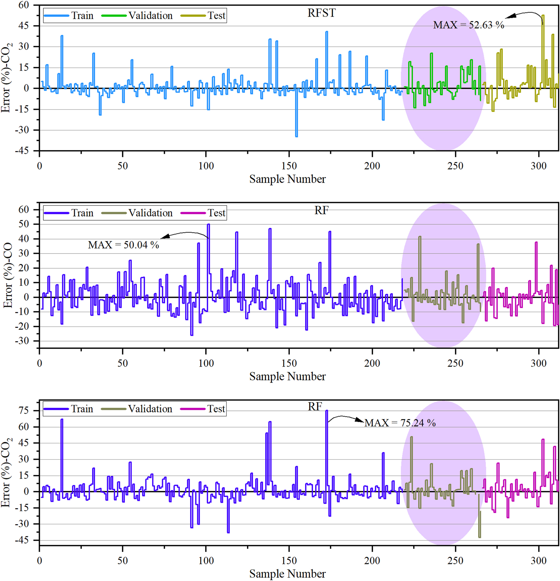
The error percentage of the models is based on the vertical plot.
In Figure 7, there is the violin with box plot errors of proposed models developed for CO and CO2. Figure 7 displays the RFJS model’s performance, with most of the samples falling in the −20 to 30 range and the distribution being relatively narrow. The RFST model’s performance is shown in Figure 7, with the majority of samples falling within an error range of −30 to 40. When it comes to CO2, it can be concluded that RFJS performed better than the other models.

The violin with box plot errors of proposed models.
The size of the particles in a gasification process can affect the amount of carbon monoxide (CO) emissions produced [52]. This is because the amount of oxygen available for the combustion reaction can vary depending on the particle size, which affects the amount of unburned fuel and incomplete combustion [29]. Overall, with smaller particle sizes, the higher the CO may result because of a greater proportion of surface to volume and possibly an insufficient amount of oxygen for the complete combustion process. Larger particle sizes will be less likely to have that high of a surface area-to-volume ratio and therefore can yield a more efficient combustion process, releasing less CO. Besides feedstock, the characteristics of the produced syngas can be constrained based on other variables, such as the gasification process and even the type of feedstock used. Gasification consists of using carbon as a fuel and reacting it with either oxygen or steam to form a gas mixture product, composed of carbon monoxide (CO) among others [5]. CO output is based on the amount of carbon feed and gasification conditions involved, such as pressure, temperature, and oxygen/carbon or steam/carbon ratio. CO emissions can be higher by increasing the carbon feeding rate into the gasifier, although there exist ways to control and suppress such emissions accordingly [53]. These strategies include the improvement of gasification conditions, biomass feedstock, post-gasification treatment, and high-temperature gas cleaning with the addition of CO2 capture and storage. This results in lower CO emissions with higher hydrogen production via gasification. However, this reduction in CO emission could again depend upon factors like gasification technology, feedstock composition, operation variables, and downstream gas cleaning systems. Conditions and many other factors prevail in the effect of nitrogen on carbon monoxide emissions in gasification processes [54]. When nitrogen acts as an agent in gasification for solid fuels, it reduces oxygen concentration in the reaction zone, thereby giving rise to incomplete combustion with high levels of CO emissions. When gasification with pure oxygen or air with a high content of oxygen is carried out, nitrogen can catalyze the formation of CO through the reaction of nitrogen with carbon and the subsequent production of nitric oxide (NO). Moreover, the effect of nitrogen on CO emission would depend upon many factors like fuel type, temperature, pressure, and gas residence time. Gasification parameters need to be optimized for maximum fuel conversion efficiency with minimum CO emission. The behavior of sulfur in affecting CO emissions in gasification processes varies. The sulfur in the feedstock can get converted into sulfur compounds during gasification, and these may further react with CO to produce more CO2 [55]. If, on the other hand, a gasification process cannot adequately cope with sulfur, the presence of this agent will have negative effects, including equipment fouling or corrosion, reducing process efficiency, and increasing CO emissions. Certain gasification systems may emit more CO when sulfur is present because sulfur interferes with reactions that form other useful products. The effects of sulfur on CO emission, therefore, depend on several factors including feedstock type, design of gasification system, and sulfur by-products handling. During gasification processes, the reaction between oxygen and carbon-containing fuel leads to a generation of CO and other gases [56]. Therefore, the amount of oxygen consumed in the process of gasification directly impacts the amount of CO produced. For example, in the process of gasification, the application of more oxygen is bound to decrease the emission of CO because more oxygen will be in combination with carbon and end up forming CO2 rather than CO. Conversely, the excess oxygen results in incomplete combustion processes, hence causing the creation of NOx and other pollutants. Therefore, the quantity of oxygen to be utilized in the process of gasification will depend on factors such as fuel types used, conditions of gasification, and desired output gases. Optimization of these variables with due care can lead to an efficient and clean gasification process. Ash in the input fuel could affect the amount of CO emissions during the gasification process [57]. Ash comprises non-burnable substances that stay after the fuel has been combusted [58]. Since it can be present in gasification, it may lead to clinkering and slagging which could affect gas quality. Clinkering and slagging refer to the hard and glassy substances together with viscous remains that clog the airflow through the gasifier, interfere with the continuous process of gasification, and result in the deterioration of gas quality. Furthermore, the presence of ash in the fuel can start char particle creation during gasification. Char is a carbonaceous material that may be created by incomplete combustion of the fuel; it reacts with carbon dioxide or steam and produces CO emissions. Thus, ash can increase CO emissions during gasification. To lessen the effects of ash on CO emissions and gasification, fuel preparation methods like washing or pelletizing can be executed to reduce ash content and enhance fuel quality, and gasification technology can be devised to manage fuel with excessive ash content. The level of moisture content in gasification processes can affect the resulting CO emissions [59]. When fuel with high moisture content is used, some energy meant to produce synthesis gas evaporates water instead. Incomplete conversion of the fuel can occur as a result, leading to more CO emissions. The moisture present can also increase water vapor, which can react with carbon to form CO and H2 and, eventually, other hydrocarbons. However, if the temperature and residency in the gasifier are inadequate, the product gas may retain CO, causing higher emissions. Hence, controlling moisture content in gasification processes is essential in minimizing CO emissions. The amount of volatile matter in the fuel used for gasification has a significant effect on the amount of CO emissions [60]. When solid fuels are burned, gaseous materials are released that contain hydrogen, methane, carbon monoxide, and other volatile hydrocarbons. Gasification involves partially burning the fuel in a low-oxygen, high-temperature environment to make a gas called syngas consisting mostly of carbon monoxide and hydrogen. If there is a lot of volatile matter in the fuel, more carbon monoxide will be produced during gasification because the carbon in the volatile matter turns into carbon monoxide. Cellulose is a type of carbohydrate made up of glucose units and is typically used as a biomass feedstock for gasification [61]. Gasification of cellulose results in the production of syngas, which includes CO, H2, CO2, and trace amounts of other gases like CH4 and H2O. CO emissions during gasification are affected by several factors, including the operating temperature, residence time, and oxygen availability. Higher gas yields with lower CO and higher H2 concentrations can be achieved by increasing the temperature and residence time of the gasifier, while incomplete biomass combustion due to insufficient oxygen can result in higher CO emissions. Therefore, efficient and low-emission syngas are produced at the optimum gasifier operating conditions. Cellulose input was dependent on these variables concerning CO emissions. Hemicellulose accounted for most of the main biomass composition and showed the most pronounced effect in producing CO from gasification processes [62]. Hemicellulose breaks down into small molecules during gasification as CO, CO2, and hydrogen-thus contributing to the overall CO output from the process. The presence of hemicellulose would also impact the temperature and residence time for complete gasification and the composition and quality of the synthesis gas produced. In general, the increased temperatures and longer residence times result in less CO emission, while lower temperatures and shorter residence times might lead to incomplete gasification and high CO emissions. Briefly, hemicellulose is a complex feedstock for CO emissions, depending on variables such as biomass feedstock specifics, gasification technology, or operating conditions of the process.
3.1 Limitations
Some of the main challenges that the proposed machine learning approach, based on the RF model optimized by JSO and STOA, has to be considered for real-world applications, are: high computational power required for model training and optimization, often impossible to provide with standard hardware, and cloud solutions or access to some other form of advanced hardware; large datasets necessary for the effectiveness of the model, which can be difficult to obtain when trying to capture a variety of operating conditions in gasification processes. Poor data quality and variability affect the performance of the model also; inaccurate data collection and noise may lower the accuracy. Random Forest models are difficult to interpret, which presents a problem in certain cases where clear insights for stakeholders may be necessary, for instance, for regulatory purposes. Moreover, the scalability of the model demands its retraining and adaptation to the change in conditions. Most importantly, integration within the existing systems requires collaboration among several professionals to assure compatibility. Meeting these challenges will be crucial for the successful deployment and effective use of machine learning in gasification processes and environmental applications.
3.2 Future study
Further studies should be directed to certain key areas that can further enhance the machine-learning approach in bringing out better improvements in gasification systems. Namely, the development of more accurate hybrid models by incorporating advanced techniques such as deep learning and the investigation of optimization algorithms including PSO and GA can substantially improve the performance. Applications of these models to real-time control of gasification processes will facilitate dynamic changes for minimum emissions. The scope could be further expanded to predict other greenhouse gases, such as methane (CH₄), for a more holistic environmental review. Integration with more sophisticated sensor technologies for continuous monitoring could further improve data acquisition and prediction accuracy. Long-term performance monitoring and an adaptive learning system in development would assure the reliability of the models over time. Finally, the assessment of economic implications from these machine learning models would support comparisons of cost-effectiveness and their impact on emissions reduction. These directions are suggested to enhance the applicability and efficiency of machine learning in gasification process optimization toward better environmental performance.
4 Conclusions
These findings from the study illustrate that machine learning can indeed be a very powerful technique in modeling Carbon Monoxide and Carbon Dioxide emissions in gasification, probably because hidden relationships and correlations in gasification data could become easily exposed. It enables the development of predictive models that are capable of optimizing the gasification process to reduce emissions with optimized machine-learning techniques like RFJS and RFST. In fact, among the others, the RF+JSO model had the best performance in CO₂ prediction for all data sets considered, since it was characterized by the lowest RMSE on the test set at 0.593, the best R 2 on the validation set, and the highest VAF on the training set at 0.983. Thus, these results confirm that RFJS is the most reliable model in emission predictions since it guarantees a high score of precision in both the CO validation and testing phases and an accuracy comparable to CO₂. While RFST and standalone RF models also performed well, with lower absolute error values than RFJS on validation and test sets, they exhibited slightly lower overall predictive accuracy. The negative BIAS values across all models suggest a minor tendency to underpredict the target variable. In conclusion, the RFJS model emerges as the optimal choice for this emission modeling task, yet all models showed strong predictive capability. Additionally, the use of machine learning in gasification emissions modeling has broader implications: it enables the identification of improvement areas within equipment and processes and can guide the design of more effective gas-cleaning systems, such as scrubbers or filters, that reduce CO and CO₂ emissions from syngas. Ultimately, these predictive models provide actionable insights to support cleaner and more efficient energy production methods.
Funding source: Research and develpment of data managment integration for intllegent control equipment of Industrial wastewater treatment based on deep learning algorithm
Award Identifier / Grant number: KYP022204
Acknowledgments
I would like to take this opportunity to acknowledge that there are no individuals or organizations that require acknowledgment for their contributions to this work.
-
Research ethics: Research involving Human Participants and Animals: the observational study conducted on medical staff needs no ethical code. Therefore, the above study was not required to acquire ethical code.
-
Informed consent: This option is not neccessary due to that the data were collected from the references.
-
Author contributions: All authors contributed to the study’s conception and design. Data collection, simulation and analysis were performed by “Baohua Shen, Xiaoman Lu, Juan Jiang and Daoguo Li”. The first draft of the manuscript was written by “Xiaoman Lu” and all authors commented on previous versions of the manuscript. All authors have read and approved the manuscript.
-
Use of Large Language Models, AI and Machine Learning Tools: During the preparation of this work, the authors used ChatGPT by OpenAI and Grammarly in order to assist with language refinement and ensure clarity and coherence in the manuscript, and perform grammar and spell checks. After using these tools/services, the authors reviewed and edited the content as needed and take full responsibility for the content of the published article.
-
Conflict of interest: The authors declare no competing interests.
-
Research funding: This work was supported by Research and develpment of data managment integration for intllegent control equipment of Industrial wastewater treatment based on deep learning algorithm (KYP022204).
-
Data availability: The authors do not have permission to share data.
References
1. Hameed, Z, Aslam, M, Khan, Z, Maqsood, K, Atabani, AE, Ghauri, M, et al.. Gasification of municipal solid waste blends with biomass for energy production and resources recovery: current status, hybrid technologies and innovative prospects. Renew Sustain Energy Rev 2021;136:110375. https://doi.org/10.1016/j.rser.2020.110375.Search in Google Scholar
2. Floudas, CA, Elia, JA, Baliban, RC. Hybrid and single feedstock energy processes for liquid transportation fuels: a critical review. Comput Chem Eng 2012;41:24–51. https://doi.org/10.1016/j.compchemeng.2012.02.008.Search in Google Scholar
3. Dimitriou, I, García-Gutiérrez, P, Elder, RH, Cuéllar-Franca, RM, Azapagic, A, Allen, RWK. Carbon dioxide utilisation for production of transport fuels: process and economic analysis. Energy Environ Sci 2015;8:1775–89. https://doi.org/10.1039/c4ee04117h.Search in Google Scholar
4. Faaij, A, Van Ree, R, Waldheim, L, Olsson, E, Oudhuis, A, Van Wijk, A, et al.. Gasification of biomass wastes and residues for electricity production. Biomass Bioenergy 1997;12:387–407. https://doi.org/10.1016/s0961-9534(97)00010-x.Search in Google Scholar
5. Beagle, E, Wang, Y, Bell, D, Belmont, E. Co-gasification of pine and oak biochar with sub-bituminous coal in carbon dioxide. Bioresour Technol 2018;251:31–9. https://doi.org/10.1016/j.biortech.2017.12.027.Search in Google Scholar PubMed
6. Asadullah, M. Barriers of commercial power generation using biomass gasification gas: a review. Renew Sustain Energy Rev 2014;29:201–15. https://doi.org/10.1016/j.rser.2013.08.074.Search in Google Scholar
7. Pereira, EG, Da Silva, JN, de Oliveira, JL, Machado, CS. Sustainable energy: a review of gasification technologies. Renew Sustain Energy Rev 2012;16:4753–62. https://doi.org/10.1016/j.rser.2012.04.023.Search in Google Scholar
8. Ramos, A, Monteiro, E, Rouboa, A. Numerical approaches and comprehensive models for gasification process: a review. Renew Sustain Energy Rev 2019;110:188–206. https://doi.org/10.1016/j.rser.2019.04.048.Search in Google Scholar
9. Mahinpey, N, Gomez, A. Review of gasification fundamentals and new findings: reactors, feedstock, and kinetic studies. Chem Eng Sci 2016;148:14–31. https://doi.org/10.1016/j.ces.2016.03.037.Search in Google Scholar
10. AlNouss, A, McKay, G, Al-Ansari, T. A techno-economic-environmental study evaluating the potential of oxygen-steam biomass gasification for the generation of value-added products. Energy Convers Manag 2019;196:664–76. https://doi.org/10.1016/j.enconman.2019.06.019.Search in Google Scholar
11. Inayat, M, Sulaiman, SA, Kurnia, JC, Shahbaz, M. Effect of various blended fuels on syngas quality and performance in catalytic co-gasification: a review. Renew Sustain Energy Rev 2019;105:252–67. https://doi.org/10.1016/j.rser.2019.01.059.Search in Google Scholar
12. Mondal, P, Dang, GS, Garg, MO. Syngas production through gasification and cleanup for downstream applications—recent developments. Fuel Process Technol 2011;92:1395–410. https://doi.org/10.1016/j.fuproc.2011.03.021.Search in Google Scholar
13. Chanthakett, A, Arif, MT, Khan, MMK, Oo, AMT. Performance assessment of gasification reactors for sustainable management of municipal solid waste. J Environ Manage 2021;291:112661. https://doi.org/10.1016/j.jenvman.2021.112661.Search in Google Scholar PubMed
14. Janajreh, I, Adeyemi, I, Raza, SS, Ghenai, C. A review of recent developments and future prospects in gasification systems and their modeling. Renew Sustain Energy Rev 2021;138:110505. https://doi.org/10.1016/j.rser.2020.110505.Search in Google Scholar
15. Islam, MW. Effect of different gasifying agents (steam, H2O2, oxygen, CO2, and air) on gasification parameters. Int J Hydrogen Energy 2020;45:31760–74. https://doi.org/10.1016/j.ijhydene.2020.09.002.Search in Google Scholar
16. Ozbas, EE, Aksu, D, Ongen, A, Aydin, MA, Ozcan, HK. Hydrogen production via biomass gasification, and modeling by supervised machine learning algorithms. Int J Hydrogen Energy 2019;44:17260–8. https://doi.org/10.1016/j.ijhydene.2019.02.108.Search in Google Scholar
17. Bahadar, A, Kanthasamy, R, Sait, HH, Zwawi, M, Algarni, M, Ayodele, BV, et al.. Elucidating the effect of process parameters on the production of hydrogen-rich syngas by biomass and coal Co-gasification techniques: a multi-criteria modeling approach. Chemosphere 2022;287:132052. https://doi.org/10.1016/j.chemosphere.2021.132052.Search in Google Scholar PubMed
18. Zhang, Z, Bai, J, Li, S, Liu, Y, Li, C, Zhong, X, et al.. Optimization of coal gasification process based on a dynamic model management strategy. J Taiwan Inst Chem Eng 2022;131:104185. https://doi.org/10.1016/j.jtice.2021.104185.Search in Google Scholar
19. Fang, Y, Ma, L, Yao, Z, Li, W, You, S. Process optimization of biomass gasification with a Monte Carlo approach and random forest algorithm. Energy Convers Manag 2022;264:115734. https://doi.org/10.1016/j.enconman.2022.115734.Search in Google Scholar
20. Kartal, F, Dalbudak, Y, Özveren, U. Prediction of thermal degradation of biopolymers in biomass under pyrolysis atmosphere by means of machine learning. Renew Energy 2023;204:774–87. https://doi.org/10.1016/j.renene.2023.01.017.Search in Google Scholar
21. Elmaz, F, Yücel, Ö, Mutlu, AY. Predictive modeling of biomass gasification with machine learning-based regression methods. Energy 2020;191:116541. https://doi.org/10.1016/j.energy.2019.116541.Search in Google Scholar
22. Hasanzadeh, R, Mojaver, P, Azdast, T, Khalilarya, S, Chitsaz, A. Developing gasification process of polyethylene waste by utilization of response surface methodology as a machine learning technique and multi-objective optimizer approach. Int J Hydrogen Energy 2023;48:5873–86. https://doi.org/10.1016/j.ijhydene.2022.11.067.Search in Google Scholar
23. Ascher, S, Watson, I, You, S. Machine learning methods for modelling the gasification and pyrolysis of biomass and waste. Renew Sustain Energy Rev 2022;155:111902. https://doi.org/10.1016/j.rser.2021.111902.Search in Google Scholar
24. Çıtmacı, B, Luo, J, Jang, JB, Morales-Guio, CG, Christofides, PD. Machine learning-based ethylene and carbon monoxide estimation, real-time optimization, and multivariable feedback control of an experimental electrochemical reactor. Chem Eng Res Des 2023;191:658–81. https://doi.org/10.1016/j.cherd.2023.02.003.Search in Google Scholar
25. Bai, FJJS. A machine learning approach for carbon di oxide and other emissions characteristics prediction in a low carbon biofuel-hydrogen dual fuel engine. Fuel 2023;341:127578. https://doi.org/10.1016/j.fuel.2023.127578.Search in Google Scholar
26. Zhao, S, Li, J, Chen, C, Yan, B, Tao, J, Chen, G. Interpretable machine learning for predicting and evaluating hydrogen production via supercritical water gasification of biomass. J Clean Prod 2021;316:128244. https://doi.org/10.1016/j.jclepro.2021.128244.Search in Google Scholar
27. George, J, Arun, P, Muraleedharan, C. Assessment of producer gas composition in air gasification of biomass using artificial neural network model. Int J Hydrogen Energy 2018;43:9558–68. https://doi.org/10.1016/j.ijhydene.2018.04.007.Search in Google Scholar
28. Li, Y, Yang, B, Yan, L, Gao, W. Neural network modeling of biomass gasification for hydrogen production. Energy Sources, Part A Recover Util Environ Eff 2019;41:1336–43. https://doi.org/10.1080/15567036.2018.1548512.Search in Google Scholar
29. Arena, U, Di Gregorio, F. Gasification of a solid recovered fuel in a pilot scale fluidized bed reactor. Fuel 2014;117:528–36. https://doi.org/10.1016/J.FUEL.2013.09.044.Search in Google Scholar
30. Franco, C, Pinto, F, Gulyurtlu, I, Cabrita, I. The study of reactions influencing the biomass steam gasification process☆. Fuel 2003;82:835–42, https://doi.org/10.1016/s0016-2361(02)00313-7.Search in Google Scholar
31. Song, T, Wu, J, Shen, L, Xiao, J. Experimental investigation on hydrogen production from biomass gasification in interconnected fluidized beds. Biomass Bioenergy 2012;36:258–67. https://doi.org/10.1016/J.BIOMBIOE.2011.10.021.Search in Google Scholar
32. Biagini, E, Barontini, F, Tognotti, L. Development of a bi-equilibrium model for biomass gasification in a downdraft bed reactor. Bioresour Technol 2016;201:156–65. https://doi.org/10.1016/J.BIORTECH.2015.11.057.Search in Google Scholar
33. Arena, U, Zaccariello, L, Mastellone, ML. Fluidized bed gasification of waste-derived fuels. Waste Manag 2010;30:1212–9. https://doi.org/10.1016/J.WASMAN.2010.01.038.Search in Google Scholar
34. Baratieri, M, Pieratti, E, Nordgreen, T, Grigiante, M. Biomass gasification with dolomite as catalyst in a small fluidized bed experimental and modelling analysis. Waste and Biomass Valorization 2010;1:283–91. https://doi.org/10.1007/S12649-010-9034-6/METRICS.Search in Google Scholar
35. Luo, S, Zhou, Y, Yi, C. Syngas production by catalytic steam gasification of municipal solid waste in fixed-bed reactor. Energy 2012;44:391–5. https://doi.org/10.1016/J.ENERGY.2012.06.016.Search in Google Scholar
36. Khan, Z, Yusup, S, Ahmad, MM, Chin, BLF. Hydrogen production from palm kernel shell via integrated catalytic adsorption (ICA) steam gasification. Energy Convers Manag 2014;87:1224–30. https://doi.org/10.1016/J.ENCONMAN.2014.03.024.Search in Google Scholar
37. Wang, J, Cheng, G, You, Y, Xiao, B, Liu, S, He, P, et al.. Hydrogen-rich gas production by steam gasification of municipal solid waste (MSW) using NiO supported on modified dolomite. Int J Hydrogen Energy 2012;37:6503–10. https://doi.org/10.1016/J.IJHYDENE.2012.01.070.Search in Google Scholar
38. Karatas, H, Akgun, F. Experimental results of gasification of walnut shell and pistachio shell in a bubbling fluidized bed gasifier under air and steam atmospheres. Fuel 2018;214:285–92. https://doi.org/10.1016/J.FUEL.2017.10.061.Search in Google Scholar
39. Van Huynh, C, Kong, S-C. Performance characteristics of a pilot-scale biomass gasifier using oxygen-enriched air and steam. Fuel 2013;103:987–96. https://doi.org/10.1016/j.fuel.2012.09.033.Search in Google Scholar
40. Yin, R, Liu, R, Wu, J, Wu, X, Sun, C, Wu, C. Influence of particle size on performance of a pilot-scale fixed-bed gasification system. Bioresour Technol 2012;119:15–21. https://doi.org/10.1016/J.BIORTECH.2012.05.085.Search in Google Scholar
41. Desai, K, Dharaskar, S, Pandya, J, Shinde, S, Vakharia, V. Experimental investigation and validation of ultrasound-assisted extractive/oxidative desulfurization of oil using environmentally benign ionic liquid. Process Saf Environ Protect 2022;166:512–23. https://doi.org/10.1016/j.psep.2022.08.029.Search in Google Scholar
42. Oyedele, O. Determining the optimal number of folds to use in a K-fold cross-validation: a neural network classification experiment. Results Math 2023;10:2201015. https://doi.org/10.1080/27684830.2023.2201015.Search in Google Scholar
43. Ascher, S, Sloan, W, Watson, I, You, S. A comprehensive artificial neural network model for gasification process prediction. Appl Energy 2022;320:119289. https://doi.org/10.1016/j.apenergy.2022.119289.Search in Google Scholar
44. Liu, D, Sun, K. Random forest solar power forecast based on classification optimization. Energy 2019;187:115940. https://doi.org/10.1016/j.energy.2019.115940.Search in Google Scholar
45. Ying, X. An overview of overfitting and its solutions. J Phys Conf Ser 2019, 1168:22022. https://doi.org/10.1088/1742-6596/1168/2/022022.Search in Google Scholar
46. Dewi, C, Chen, R-C. Random forest and support vector machine on features selection for regression analysis. Int J Innov Comput Inf Control 2019;15:2027–37.Search in Google Scholar
47. Liu, Y. Random forest algorithm in big data environment. Comput Model N Technol 2014;18:147–51.Search in Google Scholar
48. Salam, MA, Ahmed, NN, Elshamy, A, Hassan, AWS, Sami, M. Enhanced jellyfish search optimizer for collaborative team formation in social network. Int J Intell Eng Syst 2023;16.10.22266/ijies2023.0430.07Search in Google Scholar
49. Hamad, MW, Mitras, BA. A novel hybrid sooty tern optimization algorithm based on arithmetic optimization algorithm and conjugate gradient to solve optimization problems. AIP Conf Proc 2023, 2834. https://doi.org/10.1063/5.0162043.Search in Google Scholar
50. Nair, P, Vakharia, V, Shah, M, Kumar, Y, Woźniak, M, Shafi, J, et al.. AI-Driven digital twin model for reliable lithium‐ion battery discharge capacity predictions. Int J Intell Syst 2024;2024:8185044. https://doi.org/10.1155/2024/8185044.Search in Google Scholar
51. Shah, M, Borade, H, Sanghavi, V, Purohit, A, Wankhede, V, Vakharia, V. Enhancing tool wear prediction accuracy using Walsh–Hadamard transform, DCGAN and dragonfly algorithm-based feature selection. Sensors 2023;23:3833. https://doi.org/10.3390/s23083833.Search in Google Scholar PubMed PubMed Central
52. Umenweke, GC, Afolabi, IC, Epelle, EI, Okolie, JA. Machine learning methods for modeling conventional and hydrothermal gasification of waste biomass: a review. Bioresour Technol Rep 2022;17:100976. https://doi.org/10.1016/j.biteb.2022.100976.Search in Google Scholar
53. Siwal, SS, Zhang, Q, Sun, C, Thakur, S, Gupta, VK, Thakur, VK. Energy production from steam gasification processes and parameters that contemplate in biomass gasifier–A review. Bioresour Technol 2020;297:122481. https://doi.org/10.1016/j.biortech.2019.122481.Search in Google Scholar PubMed
54. Nadaleti, WC, Przybyla, G. NOx, CO and HC emissions and thermodynamic-energetic efficiency of an SI gas engine powered by gases simulated from biomass gasification under different H2 content. Int J Hydrogen Energy 2020;45:21920–39. https://doi.org/10.1016/j.ijhydene.2020.05.193.Search in Google Scholar
55. Mavukwana, A, Burra, KG, Sempuga, C, Castaldi, M, Gupta, AK. Effect of gypsum waste inclusion on syngas production during CO2-assisted gasification of waste tires. Waste Manag 2023;171:375–81. https://doi.org/10.1016/j.wasman.2023.09.022.Search in Google Scholar PubMed
56. Zhao, J, Xie, D, Wang, S, Zhang, R, Wu, Z, Meng, H, et al.. Hydrogen-rich syngas produced from co-gasification of municipal solid waste and wheat straw in an oxygen-enriched air fluidized bed. Int J Hydrogen Energy 2021;46:18051–63. https://doi.org/10.1016/j.ijhydene.2021.02.137.Search in Google Scholar
57. Valdés, CF, Marrugo, GP, Chejne, F, Marin-Jaramillo, A, Franco-Ocampo, J, Norena-Marin, L. Co-gasification and co-combustion of industrial solid waste mixtures and their implications on environmental emissions, as an alternative management. Waste Manag 2020;101:54–65. https://doi.org/10.1016/j.wasman.2019.09.037.Search in Google Scholar PubMed
58. Wang, K, Nakakubo, T. Comparative assessment of waste disposal systems and technologies with regard to greenhouse gas emissions: a case study of municipal solid waste treatment options in China. J Clean Prod 2020;260:120827. https://doi.org/10.1016/j.jclepro.2020.120827.Search in Google Scholar
59. Yan, B, Jiao, L, Li, J, Zhu, X, Ahmed, S, Chen, G. Investigation on microwave torrefaction: parametric influence, TG-MS-FTIR analysis, and gasification performance. Energy 2021;220:119794. https://doi.org/10.1016/j.energy.2021.119794.Search in Google Scholar
60. Sagi, O, Rokach, L. Approximating XGBoost with an interpretable decision tree. Inf Sci 2021;572:522–42. https://doi.org/10.1016/j.ins.2021.05.055.Search in Google Scholar
61. Mishra, K, Siwal, SS, Saini, AK, Thakur, VK. Recent update on gasification and pyrolysis processes of lignocellulosic and algal biomass for hydrogen production. Fuel 2023;332:126169. https://doi.org/10.1016/j.fuel.2022.126169.Search in Google Scholar
62. Wang, S, Zou, C, Yang, H, Lou, C, Cheng, S, Peng, C, et al.. Effects of cellulose, hemicellulose, and lignin on the combustion behaviours of biomass under various oxygen concentrations. Bioresour Technol 2021;320:124375. https://doi.org/10.1016/j.biortech.2020.124375.Search in Google Scholar PubMed
© 2024 the author(s), published by De Gruyter
This work is licensed under the Creative Commons Attribution 4.0 International License.
Articles in the same Issue
- Frontmatter
- Research Articles
- Comparative study of deterministic and stochastic optimization algorithms applied to the absorption of CO2 by alkanolamine solution
- Modeling the kinetics, energy consumption and shrinkage of avocado pear pulp during drying in a microwave assisted dryer
- Study of municipal solid waste treatment using plasma gasification by application of Aspen Plus
- Numerical analysis of segregation of microcrystalline cellulose powders from a flat bottom silo with various orifice positions
- Prediction of syngas production in the gasification process of biomass employing adaptive neuro-fuzzy inference system along with meta-heuristic algorithms
- Industrial high saline water desalination by activated carbon in a packed column- an experimental and CFD study
- Dual-loop PID control strategy for ramp tracking and ramp disturbance handling for unstable CSTRs
- A control perspective on hybrid membrane/distillation propane/propylene separation process
- Prediction of surface heating effect on non-equilibrium homogeneous condensation in supersonic nozzle using CFD method
- Modeling the emitted carbon dioxide and monoxide gases in the gasification process using optimized hybrid machine learning models