Geometry of transcendental singularities of complex analytic functions and vector fields

Alvaro Alvarez-Parrilla; Jesús Muciño-Raymundo

doi:10.1515/coma-2024-0005

Article Open Access

Geometry of transcendental singularities of complex analytic functions and vector fields

Alvaro Alvarez-Parrilla and Jesús Muciño-Raymundo

Published/Copyright: August 28, 2024

Published by

Become an author with De Gruyter Brill

Submit Manuscript Author Information Explore this Subject

From the journal Complex Manifolds Volume 11 Issue 1

Abstract

On Riemann surfaces M , there exists a canonical correspondence between a possibly multivalued function Ψ X whose differential is single-valued (i.e. an additively automorphic singular complex analytic function) and a vector field X . From the point of view of vector fields, the singularities that we consider are zeros, poles, isolated essential singularities, and accumulation points of the above. The theory of singularities of the inverse function Ψ X ‒ 1 is extended from meromorphic functions to additively automorphic singular complex analytic functions. The main contribution is a complete characterization of when a singularity of Ψ X − 1 is algebraic, is logarithmic, or arises from a zero with non-zero residue of X . Relationships between analytical properties of Ψ X , singularities of Ψ X − 1 and singularities of X are presented. Families and sporadic examples showing the geometrical richness of vector fields on the neighbourhoods of the singularities of Ψ X − 1 are studied. As applications, we have; a description of the maximal univalence regions for complex trajectory solutions of a vector field X , a geometric characterization of the incomplete real trajectories of a vector field X , and a description of the singularities of the vector field associated with the Riemann ξ -function.

Keywords: complex analytic vector fields; Riemann surfaces; essential singularities; transcendental singularities

MSC 2010: 32S65; 58K45; 30F25; 30D30; 30D20

1 Introduction

Essential singularities of meromorphic functions Ψ on C are a natural source of intricate/complex behaviour in analysis, iteration of functions, and differential equations, among other topics. From a geometrical point of view, in 1914, Iversen [25] introduced the ideal points associated with a singularity of the inverse function Ψ − 1 by defining neighbourhoods U a ( ρ ) ⊂ C , where a ∈ C ^ t is a singular value (i.e. a critical or an asymptotic value of Ψ ). Recently, Bergweiler and Eremenko have contributed in this direction, mostly applying their work to holomorphic dynamics [8,14]. A great part of the complexity of an essential singularity is that its description can require several ideal points, each with different behaviour. For meromorphic functions Ψ , the ideal points are analytically classified as follows:

algebraic singularities of the inverse function Ψ − 1 and
transcendental singularities of the inverse function Ψ − 1 .

We wish to extend this geometric perspective, more precisely the study via ideal points to not necessarily isolated essential singularities of the following:

vector fields X and, as a natural consequence,
certain multivalued functions Ψ X associated with X .

Our framework is as follows. Let M be a connected, not necessarily compact, Riemann surface. By definition, a singular complex analytic function Ψ X : M ⟶ C ^ t can admit accumulations of zeros, poles, and/or essential singularities. Throughout the work, singular complex analytic means the analogous properties for vector fields and 1-forms on M . In addition, Ψ X is additively automorphic when its differential d Ψ X is a singular complex analytic 1-form on M . Note that if Ψ X is additively automorphic, then it can be single or multivalued. The adjectives single-valued and multivalued shall be understood in the strict sense. Thus, the concept of additively automorphic singular complex analytic function Ψ X makes sense and includes the meromorphic case.

We recall the natural correspondence, which will be used throughout the work, between a function, a vector field, and an associated Riemann surface. Let Ψ X : M ⟶ C ^ t be an additively automorphic singular complex analytic function. The singular complex analytic vector field X on M canonically associated with Ψ X is defined by d Ψ X ( X ) ≡ 1 , see Diagram 7 and Section 2. Conversely, given a complex analytic vector field X , the associated Ψ X is a (generically multivalued) additively automorphic singular complex analytic function. The third element in the correspondence is the Riemann surface ℛ X ⊂ M × C ^ t , roughly speaking the graph of Ψ X .

The differential d Ψ X is the 1-form of time of X. By definition, the residue of X at a point is the residue of the 1-form of time d Ψ X at the point. In particular, Ψ X is single-valued if and only if d Ψ X has all its residues and periods^[1] equal to zero. For technical reasons, throughout the entire work, we require that the set of points where the 1-form of time d Ψ X has non-zero residues be numerable.

The classical theory of singularities of the inverse function Ψ X − 1 fails for multivalued additively automorphic singular complex analytic functions. As a simple example, consider a zero of X with non-zero residue which gives origin to an essential singularity of Ψ X − 1 at the singular value ∞ ∈ C ^ t . Thus, by the classical Casorati-Weierstrass theorem, the image of any neighbourhood of ∞ ∈ C ^ t is dense in M , i.e. the neighbourhoods U ∞ ( ρ ) are not useful in order to distinguish ideal points.

As a valuable central result, in Section 3.2, we extend Iversen’s theory to also hold for additively automorphic singular complex analytic functions Ψ X , by introducing the fundamental domain Λ of Ψ X , which is essentially a maximal univalence region for Ψ X .

The usefulness of vector fields X in the study of functions Ψ X can be roughly stated as follows. The vector field distinguishes the finite and infinite singular values a ∈ C ^ t of Ψ X and its ideal points U a in a clear geometric way. A natural/heuristic idea of this is to exploit the phase portrait of the real part Re ( X ) . This method allows us to describe the logarithmic singularities of Ψ X − 1 in geometric terms. Namely, the exponential tracts of Ψ X can be naturally classified as elliptic and hyperbolic tracts (Figures 1, 2, and 3). This leads us to the following:

$Figure 1 (a) Elliptic tracts arise from the asymptotic value ∞ ∈ C ^ t \infty \in {\widehat{{\mathbb{C}}}}_{t} . (b) Hyperbolic tracts arise from finite asymptotic values a ∈ C ^ t a\in {\widehat{{\mathbb{C}}}}_{t} . The asymptotic values a a , ∞ \infty are represented by small red circles.$

Figure 1

(a) Elliptic tracts arise from the asymptotic value ∞ ∈ C ^ t . (b) Hyperbolic tracts arise from finite asymptotic values a ∈ C ^ t . The asymptotic values a , ∞ are represented by small red circles.

$Figure 2 Geometry of exponential vector fields. (a) For X ( z ) = e z ∂ ∂ z X\left(z)={{\rm{e}}}^{z}\frac{\partial }{\partial z} of Example 4.1, the essential singularity at ∞ ∈ C ^ z \infty \in {\widehat{{\mathbb{C}}}}_{z} gives rise to two logarithmic singularities; one hyperbolic tract over the singular value 0, and one elliptic tract over ∞ ∈ C ^ t \infty \in {\widehat{{\mathbb{C}}}}_{t} . (b) For X ( z ) = ( e z 3 ⁄ z 2 ) ∂ ∂ z X\left(z)=\left({{\rm{e}}}^{{z}^{3}}/{z}^{2})\frac{\partial }{\partial z} of Example 4.2.1, the essential singularity at ∞ ∈ C ^ z \infty \in {\widehat{{\mathbb{C}}}}_{z} gives rise to six logarithmic singularities. There are three hyperbolic tracts with finite asymptotic value 0, with multiplicity 3, and three elliptic tracts with asymptotic value ∞ \infty , accurately denoted ∞ 1 , ∞ 2 , ∞ 3 {\infty }_{1},{\infty }_{2},{\infty }_{3} . The colouring scheme for petal regions is as follows: green for hyperbolic tracts and blue for elliptic tracts, it will be used consistently throughout.$

Figure 2

Geometry of exponential vector fields. (a) For X ( z ) = e z ∂ ∂ z of Example 4.1, the essential singularity at ∞ ∈ C ^ z gives rise to two logarithmic singularities; one hyperbolic tract over the singular value 0, and one elliptic tract over ∞ ∈ C ^ t . (b) For X ( z ) = ( e z 3 ⁄ z 2 ) ∂ ∂ z of Example 4.2.1, the essential singularity at ∞ ∈ C ^ z gives rise to six logarithmic singularities. There are three hyperbolic tracts with finite asymptotic value 0, with multiplicity 3, and three elliptic tracts with asymptotic value ∞ , accurately denoted ∞ 1 , ∞ 2 , ∞ 3 . The colouring scheme for petal regions is as follows: green for hyperbolic tracts and blue for elliptic tracts, it will be used consistently throughout.

$Figure 3 Geometry of vector fields X X on C ^ z {\widehat{{\mathbb{C}}}}_{z} with an essential singularity at ∞ \infty , with accumulations of poles and/or zeros. (a) is described in Example 5.3, (b) in Example 5.5, (c) in Example 5.13, (d) in Example 5.11, (e) in Example 5.12, and (f) in Example 5.14. The colouring scheme for neighbourhoods U a ( ρ ) {U}_{a}\left(\rho ) , determining singularities of Ψ X ‒ 1 {\Psi }_{X}^{‒1} , is green for hyperbolic tracts and blue for elliptic tracts (to be described in Definition 4.1 and Figure 1). Moreover, purple region in (c) denotes a connected component U ∞ ( ρ ) {U}_{\infty }\left(\rho ) . Green and red dots represent zeros and poles of X ( z ) X\left(z) , respectively. It is remarkable, that G. Gyllström [18] describes intricate phase portraits of ordinary differential equations one century ago.$

Figure 3

Geometry of vector fields X on C ^ z with an essential singularity at ∞ , with accumulations of poles and/or zeros. (a) is described in Example 5.3, (b) in Example 5.5, (c) in Example 5.13, (d) in Example 5.11, (e) in Example 5.12, and (f) in Example 5.14. The colouring scheme for neighbourhoods U a ( ρ ) , determining singularities of Ψ X ‒ 1 , is green for hyperbolic tracts and blue for elliptic tracts (to be described in Definition 4.1 and Figure 1). Moreover, purple region in (c) denotes a connected component U ∞ ( ρ ) . Green and red dots represent zeros and poles of X ( z ) , respectively. It is remarkable, that G. Gyllström [18] describes intricate phase portraits of ordinary differential equations one century ago.

Ansatz: The ideal points or singularities of Ψ X − 1 can be understood as the points of the ideal boundary ^[2] of M minus the essential singularities and the multivalued locus of Ψ X . In other words, the ideal points are the branch points of the Riemann surface ℛ X .

Regarding the singularities of the inverse for single-valued Ψ X on M = C , the cases of algebraic and logarithmic singularities are understood best. Recall the following well-known classical result.

Theorem

(Nevanlinna, [35] Ch. XI, §1.3) A transcendental singularity of Ψ − 1 over an isolated asymptotic value is logarithmic.

We shall prove a stronger version of the above result (the if and only if assertion and the extension to the multivalued case). For this, we require the following definitions and methods suggested by the above ansatz. Roughly speaking, a ⋆ -transcendental singularity of Ψ X − 1 arises from a pole of d Ψ X with non-zero residue, see Definition 3.14. Second, a singularity U a is separate if for a small enough ρ > 0 the neighbourhood U a ( ρ ) does not intersect any other neighbourhood of another ideal point; Definition 4.2 provides full details, see Examples 5.5–5.9 in Section 5. Regarding Nevanlinna’s result, for single-valued Ψ X , a non-isolated singular value can support separate (including logarithmic) and non-separate singularities. Our result covers the single, and multivalued cases.

Theorem 4.4

(Separate singularities) Let Ψ X : M ⟶ C ^ t be an additively automorphic singular complex analytic function. A singularity U a of Ψ X − 1 is separate if and only if U a is one of the following:

algebraic,
⋆ -transcendental,
logarithmic.

Noting that the geometry^[3] of transcendental separate singularities is independent of the value of the corresponding residue, it is natural to ask: Which new phenomena appear for multivalued Ψ X ?

Using Definition 3.14, the relationship between the singularities of Ψ X − 1 and the singularities of X is the statement of Theorems 4.6 and 4.9. A rough description of the relationship is as follows:

algebraic singularity of Ψ X − 1 poles of X , P , zeros of X with residue zero, Z 0 , transcendental singularity of Ψ X − 1 zeros of X with non-zero residue, Z R , essential singularities of X with residue zero, E 0 , essential singularities of X with non-zero residue, E R , essential singularities of X w i t h o u t r e s i d u e , E n R .

The adjective without residue means that the residue of d Ψ X at the respective essential singularity is not well defined (e.g., if it is an accumulation of singularities with non-zero residue). The aforementioned relationship is far from being a bijection; an essential singularity of X gives rise to none, one or more than one transcendental singularity of Ψ X − 1 . Example 4.3 provides a singularity of X in E n R that does not allow a singularity of the inverse Ψ X − 1 . In addition, Example 5.13 provides a singularity of X in E 0 with exactly one singularity of Ψ X − 1 . Theorem 5.1 describes generic X , where an essential singularity supports and even number of singularities of Ψ X − 1 . As a fortunate coincidence,

S = P ∪ Z 0 ∪ Z R ∪ E 0 ∪ E R ∪ E n R

also refers in a uniform way to the singularities of X , ω X , and Ψ X . For example, z s ∈ P denotes a pole of X , simultaneously a zero of ω X and a critical point of Ψ X .

In Section 5, we study finite dimensional holomorphic families of additively automorphic functions Ψ X with essential singularities. The use of the fundamental domain Λ technique allows us to reduce their study to single-valued functions Ψ X , Λ . As one of the contributions of this work, the singularities of Ψ X − 1 for the multivalued case are considered for the first time in the literature. In particular, vector fields with essential singularities that are accumulation points of zeros with non-zero residue are examined.

We consider the families

E ( s , r , d ) = X ( z ) = Q ( z ) P ( z ) e E ( z ) ∂ ∂ z Q , P , E ∈ C [ z ] of degree s , r , d ≥ 1 .

Theorem 5.1 describes the associated additively automorphic functions

Ψ X ( z ) = ∫ z P ( ζ ) Q ( ζ ) e − E ( ζ ) d ζ , on C ^ z .

All the singularities of Ψ X − 1 are separate. The zeros and poles with zero residue of d Ψ X correspond to algebraic singularities of Ψ X − 1 . The poles with non-zero residue of d Ψ X correspond to ⋆ -transcendental singularities of Ψ X − 1 . The essential singularity consists of 2 d logarithmic singularities: d elliptic tracts and d hyperbolic tracts equidistributed about ∞ ∈ C ^ z .

These functions are the simplest in several deep subjects, determining functions with a finite number of singular values. They are related to the Schwartzian second-order differential equation, see [23,35] Ch. XI, and appear in the deformation of ramified coverings [44] and [45]. Also see our previous work [5] and references therein.

As second kind of families, Theorem 5.2 studies the functions

Ψ X ( z ) = R ( e 2 π i z ⁄ T ) ,

where R ( w ) are rational functions of degree r ≥ 1 , T ∈ C * . A systematic description that depends on the behaviour of R is provided. Note that this family is the simplest having periodic functions and/or vector fields where an accumulation of zeros and poles at the essential singularity ∞ appear.

In Section 5.3, the geometrical richness of the behaviour of the singularities of the inverse function Ψ X − 1 that may appear, even in the single-valued case, is explored. Examples of single-valued functions are considered from the perspective of vector fields; also examples of vector fields X which give rise to multivalued additively automorphic Ψ X are fully explained.

In Section 6, we provide three applications. In Section 6.1, we obtain a description of the maximal region for complex trajectory solutions of X , which a priori are multivalued.

Theorem 6.4

(Maximal univalence region for trajectory solutions) Let X be a singular complex analytic vector field on M. The maximal univalence region for a non-stationary complex solution z ( t ) of X is

D X = { ( z , Ψ X ( z ) ) ∣ z ∈ M \ S } .

Moreover, D X is independent of the initial condition z o ∈ M \ S .

As a second application, an incomplete trajectory of X is a solution of Re ( X ) with a strict subset of R as maximal domain of existence. Clearly, from the local analytic normal form of X , each pole p of X provides a finite number of incomplete trajectories. In Proposition 6.5, the following natural result is presented.

Every non-rational, singular complex analytic vector field X on a compact Riemann surface M g , of genus g , has an infinite number of incomplete trajectories. At a pole or essential singularity of X , the following clear mechanism occurs.

Theorem 6.7

(Incomplete trajectories and finite singular values) Let X be a singular complex analytic vector field on M . The following statements are equivalent.

There exists an incomplete trajectory z ( t ) of X having α or ω -limit at z s ∈ M .
There exists a finite singular value a ∈ C t of Ψ X , whose asymptotic path α a ( t ) is a trajectory of Re ( X ) ending at z s ∈ M .

This raises a natural question: Which neighbourhoods U a ( ρ ) of the singularities of Ψ X − 1 contain incomplete trajectories, and how many are there?

As example, the neighbourhoods U ∞ ( ρ ) of separate singularities over ∞ ∈ C ^ t do not have incomplete trajectories. An analogous problem has been recently considered by Langley [28–30]. As an application of Theorem 4.4, in Section 6.2, we prove a constructive description of how the incomplete trajectories of X on a Riemann surface M arise in a vicinity of an essential singularity.

Theorem 6.9

(Localizing incomplete trajectories) Let X be a singular complex analytic vector field on M with an essential singularity at z s ∈ M .

Any neighbourhood U a ( ρ ) , of an essential transcendental singularity U a of Ψ X − 1 over a finite asymptotic value a ∈ C t , contains an infinite number of incomplete trajectories of X.
If Ψ X has no finite asymptotic values at z s , then X has an infinite number of poles accumulating at z s ∈ M .

In other words, any neighbourhood of an essential singularity of X has an infinite number of incomplete trajectories.

As a third and final application, in Section 6.3, by recalling the work of Broughan [10] on the Riemann ξ -vector field X ξ ( z ) = ξ ( z ) ∂ ∂ z , we show that it is not holomorphically equivalent to a pullback of a periodic vector field with a finite number of distinct residues. Furthermore, we show that Ψ X ξ − 1 has two logarithmic singularities over finite asymptotic values, whose hyperbolic tracts are the left and right half planes delimited by the critical strip. In addition, Ψ X ξ − 1 has an infinite number of ⋆ -transcendental singularities over ∞ corresponding to the zeros with non-zero residue in the critical strip; see Proposition 6.14.

In Section 7, some possible avenues of further research are presented.

Finally, we make a few comments from a panoramic viewpoint:

In Riemann surface theory, all the meromorphic functions can be constructed by using the elementary blocks { z ↦ z d } , i.e. the algebraic singularities of the inverse.
Many singular complex analytic functions can be constructed by using two new elementary blocks: hyperbolic and elliptic tracts, i.e. the logarithmic singularities of the inverse.
In the general case of singular complex analytic functions, an infinite number of new blocks appear: those arising from the non-separate singularities of the inverse.
Furthermore, for multivalued functions, the ⋆ -transcendental singularities of the inverse complete the aforementioned elementary blocks.
In any case, as the examples throughout the text show, clear patterns can be recognized by using the aforementioned elementary building blocks.

2 General facts about functions and vector fields

2.1 Functions and vector fields on Riemann surfaces

Let M be a Riemann surface, not necessarily compact, if we assume that p is a conformal puncture^[4] of M , then we consider p in M . Thus, our Riemann surface M includes their conformal punctures.

Definition 2.1

On M , the adjective singular complex analytic for functions, vector fields, 1-forms, and quadratic differentials means that they may have accumulation of zeros, poles, and/or essential singularities.

The singular complex analytic category includes holomorphic and meromorphic objects on compact Riemann surfaces, which are not transcendental meromorphic: i.e. singular complex analytic is a larger class.

Definition 2.2

([7] p. 579) A multivalued or single-valued analytic function Ψ X on M is additively automorphic when its differential d Ψ X is a single-valued 1-form.

Of course any single-valued singular complex analytic function is additively automorphic; however, not all multivalued singular complex analytic functions are additively automorphic.

Notation.

An additively automorphic singular complex analytic function Ψ X on M satisfies Definitions 2.1 and 2.2.
A single-valued additively automorphic singular complex analytic function Ψ X on M is strictly single-valued.
A multivalued additively automorphic singular complex analytic function Ψ X on M is strictly multivalued.

The advantage of the subscript X is explained below.

Throughout this work, we assume that all the vector fields X are not identically zero and that the functions Ψ X are not identically constant. The formal expression of a vector field X in holomorphic charts { ϕ j : V j ⊂ M ⟶ C z } must be { f j ( z ) ∂ ∂ z ∣ z ∈ ϕ j ( V j ) } ; as far as possible, we avoid this cumbersome notation.

From additively automorphic singular complex analytic functions to singular complex analytic vector fields. Let

Ψ X : M ⟶ C ^ t

be an additively automorphic singular complex analytic function (probably not well defined at every point since we are abusing notation). Since its differential is single-valued, the canonical associated singular complex analytic vector field is

X ( z ) = 1 Ψ X ′ ( z ) ∂ ∂ z on M .

From singular complex analytic vector fields to additively automorphic singular complex analytic functions: Let

(1) X ( z ) = f ( z ) ∂ ∂ z

be a singular complex analytic vector field on M . By definition, the singular complex analytic 1-form of time of X is

(2) ω X ( z ) = d z f ( z ) .

We want to define Ψ X ( z ) = ∫ z ω X with single-valued ω X .

Remark 2.3

The residue of ω X at z 0 ∈ M ,

(3) Res ( ω X , z 0 ) = 1 2 π i ∫ γ ω X ∈ C

is well defined if and only if z 0 is

a regular point of X (as usual the counterclockwise path γ encloses z 0 and the integral is zero),
an isolated singularity of X , or
a non-isolated singularity of X which is at most an accumulation of singular points with residue zero, e.g. of poles of X (in this case the path γ encloses z 0 and those infinite number of singular points).

By definition, the residue of X at a point z 0 is the residue of ω X , i.e.

Res ( X , z 0 ) ≐ Res ( ω X , z 0 ) .

The singularities of X,

(4) S = { z s } = Z 0 ∪ Z R ︸ Z ∪ P ∪ E 0 ∪ E R ∪ E n R ︸ E ⊂ M ,

are possibly infinite, of the following kinds:

The zeros of X,

Z = { q } = Z 0 ∪ Z R ,

where Z 0 (resp. Z R ) denotes the zeros of X with residue zero (resp. with non-zero residue).

The poles of X,

P = { p } .

The essential singularities of X,

E = { e } = E 0 ∪ E R ∪ E n R ,

where E 0 (resp. E R ) denotes the essential singularities of X with residue zero (resp. with non-zero residue), and the points E n R where the residue is not well defined; these last are accumulation of points of Z R ∪ E R .

In addition, we introduce the following notations:

S 0 = Z 0 ∪ E 0 and S R = Z R ∪ E R .

Because of technical reasons, to be used in Section 3.2, we require that S R is at most a numerable set. Through all the work, S in (4) also refers to the singularities of Ψ X and ω X . For example, in accordance with equations (1) and (2), z s ∈ Z denotes a zero of X and simultaneously a pole of ω X .

Note that

M \ ( S R ¯ ∪ E 0 ) = M \ ( E ∪ Z R ) .

The additively automorphic singular complex analytic function associated with X is

(5) Ψ X ( z ) = ∫ z o z ω X : M \ ( E ∪ Z R ) ⟶ C ^ t

and the initial point of integration is a non-singular point z o ∈ M \ S ; for simplicity, we omit it in some instances.

Remark 2.4

In (5), the integral function Ψ X ( z ) is single-valued if and only if
1. the residues Res ( ω X , z s ) , for z s ∈ S , and
2. the periods ∫ β ω X , where the class [ β ] is in a basis of the fundamental group π 1 ( M ) and does not enclose an isolated singularity, are both zero.
Assertion 1.i is equivalent to S R = Z R ∪ E R = ∅ .
The multivaluedness of the integral function shall be studied in Section 3.2.

Remark 2.5

In both cases, single-valued or multivalued Ψ X is a global flow box that rectifies the corresponding singular complex analytic vector field X , thus
( Ψ X ) * X = ∂ ∂ t .
In the language of quadratic differentials, Ψ X is the global distinguished parameter of X , and we exploit the global nature. Clearly, the poles of X determine zeros of ω X and critical points of Ψ X in M .

Proposition 2.6

(Dictionary between the singular analytic objects, [3,33] §2) On a Riemann surface M, there exists a canonical correspondence between the following objects.

A singular complex analytic vector field X = f ( z ) ∂ ∂ z , as in (1).
A singular complex analytic 1-form ω X = d z ⁄ f ( z ) , as in (2).
An additively automorphic singular complex analytic function Ψ X ( z ) = ∫ z ω X as in (5).
An orientable singular complex analytic quadratic differential Q X = ω X ⊗ ω X , where the trajectories of X coincide with horizontal trajectories of Q X .
A singular flat metric g X = Ψ * ∣ d t ∣ on M , which is the pullback of the flat Riemannian metric ∣ d t ∣ = d t 2 + d s 2 , t ≐ t + i s ∈ C , having suitable singularities at S and a unitary geodesic vector field Re ( X ) . By abuse of notation, ( M , g X ) denotes this singular non-compact Riemannian manifold.
A Riemann surface ℛ X , π 2 * ( ∂ ∂ t ) associated with an additively automorphic singular complex analytic function Ψ X , where
(6) ℛ X = { ( z , t ) ∣ t = Ψ X ( z ) , z ∈ M \ ( E ∪ Z R ) } ⊂ M × C ^ t .

□

Diagrammatically,

(7)

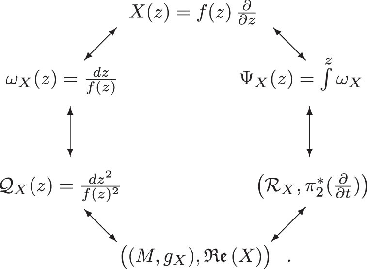
Remark 2.7

The correspondence (7) must be understood up to choice of initial point z o for the integral defining the global distinguished parameter. Thus, Ψ X and Ψ X + c , for c ∈ C , are considered the same object.

Example 2.1

(Abelian integrals)

Note that non-additively automorphic multivalued functions do not produce singular complex analytic vector fields. For instance, consider the non-additively automorphic multivalued singular complex analytic function
Θ ( z ) = ∫ z d ζ P ( ζ ) : C ^ z ⟶ C ^ t , where P ∈ C [ z ] , deg P ≥ 2 .
Obviously, P ( z ) ∂ ∂ z is not a single-valued vector field on C z . However, on the (hyper) elliptic Riemann surface M = { w 2 − P ( z ) = 0 } , the integrand d z ⁄ P ( z ) determines a holomorphic 1-form ω X , thus the Abelian integral
Ψ X ( z ) = ∫ z ω X : M ⟶ C
is an additively automorphic singular complex analytic function on M . An associated meromorphic vector field X on M is well defined.
Let ω X be a meromorphic 1-form on a compact Riemann surface M . The integral function Ψ X ( z ) = ∫ z ω X : M \ Z R ⟶ C ^ t is an additively automorphic singular complex analytic function.

Remark 2.8

Note that vector fields X with E n R ≠ ∅ are quite common, for instance, see Figure 3(d), (e), and (f) discussed in Examples 5.11, 5.13, and 5.14, where E n R is an accumulation of points of Z R in the first two cases and an accumulation of Z R ∪ P in the third case. See also Example 4.3.

Lemma 2.9

With the notation as above.

The following diagram of pairs, (Riemann surface, vector field), commutes

(8) where π 1 and π 2 are local isometric, possibly branched coverings over ( M , g X ) and ( C ^ t , ∣ d t ∣ ) as singular Riemannian manifolds, respectively.
Moreover, Ψ X is single-valued if and only if the projection π 1 is a biholomorphism between
ℛ X , π 2 * ( ∂ ∂ t ) a n d ( M \ ( E ∪ Z R ) , X ) .
The (ideal) boundary of ℛ X is totally disconnected, separable, and compact.

Proof

A proof of (3) can be found in [2] Ch. I §6, or [38] as Proposition 3.□

We shall use the abbreviated form ℛ X instead of the cumbersome ℛ X , π 2 * ( ∂ ∂ t ) .

Example 2.2

Let X be a singular complex analytic vector field on M = C ^ z .

By Lemma 2.9.2, the Riemann surface ℛ X is biholomorphic to C ^ z \ E if and only if every zero or essential singularity of X has zero residue (in symbols Z = Z 0 , E = E 0 ).
The Riemann surface ℛ X is the universal cover of C ^ z \ ( E ∪ Z ) if and only if every zero or essential singularity of X has non-zero residue (in other words Z 0 ∪ E 0 ∪ E n R = ∅ ).

Definition 2.10

A maximal real trajectory solution of X is z ( t ) : ( a , b ) ⊆ R ⟶ M \ ( P ∪ E ) , where a , b ∈ R ∪ { ∓ ∞ } , satisfying that

d z ( t ) d t = f ( z ( t ) ) , z ( 0 ) = z o ∈ M \ ( P ∪ E ) .

Equivalently, z ( t ) is a trajectory of the associated real vector field Re ( X ) .

Abusing notation, the phase portrait of X means the portrait of the real vector field Re ( X ) . Moreover, the trajectories z ( t ) of Re ( X ) coincide with the level sets

{ Im ( Ψ X ( z ) ) = c } , for c ∈ R ,

i.e. the horizontal trajectories of the orientable quadratic differential Q X . However, the inversion Ψ X − 1 ( t ) of the integral in equation (5) provides the non-stationary complex trajectory solutions of the vector field X .

There is a natural advantage of studying additively automorphic singular complex analytic functions Ψ X via the associated vector fields X , as seen in [3–5,33]. Very particular families of vector fields with one essential singularity are considered in [3–5]. Meromorphic vector fields on compact Riemann surfaces are a current subject of study, see, e.g. in [13,27] and references therein.

2.2 Local theory of vector fields

Definition 2.11

([3] §5) Let ( C ^ , ∂ ∂ z ) be the holomorphic vector field on the Riemann sphere with a double zero at ∞ , and let H ¯ 2 = { Im ( z ) ≥ 0 } ∪ { ∞ } ⊂ C ^ .

A hyperbolic sector is the vector field germ H = ( H ¯ 2 , 0 ) , ∂ ∂ z , as in Figure 4(c).
An elliptic sector is the vector field germ E = ( H ¯ 2 , ∞ ) , ∂ ∂ z , equivalently ( H ¯ 2 , 0 ) , − w 2 ∂ ∂ w when { z ↦ 1 z = w } , Figure 4(a).
A (right) parabolic sector is the vector field germ
P + = ( { 0 ≤ Im ( z ) ≤ h } ∩ { Re ( z ) > 0 } , ∞ ) , ∂ ∂ z ,
in addition the (left) parabolic sector P − occurs when Re ( z ) < 0 ; h ∈ R + is a parameter (Figure 4(b)).

$Figure 4 (a) Elliptic E E , (b) parabolic P P , and (c) hyperbolic H H sectors of Re ( X ) {\mathfrak{Re}}(X) . The left drawing sketches the sphere ( C ^ t , ∂ ∂ t ) \left({\widehat{{\mathbb{C}}}}_{t},\frac{\partial }{\partial t}) describing their embeddings under Ψ X {\Psi }_{X} .$

Figure 4

(a) Elliptic E , (b) parabolic P , and (c) hyperbolic H sectors of Re ( X ) . The left drawing sketches the sphere ( C ^ t , ∂ ∂ t ) describing their embeddings under Ψ X .

The sectors are germs of flat Riemannian manifolds with boundary provided with a complex vector field; in [3] §5, we describe their properties. Thus, we say that X has a hyperbolic, elliptic, or parabolic when Re ( X ) has it.

The following result appears in the theory of quadratic differentials [1,26,43] and in complex differential equations [9,15,19–21,34], (Figure 5).

Figure 5

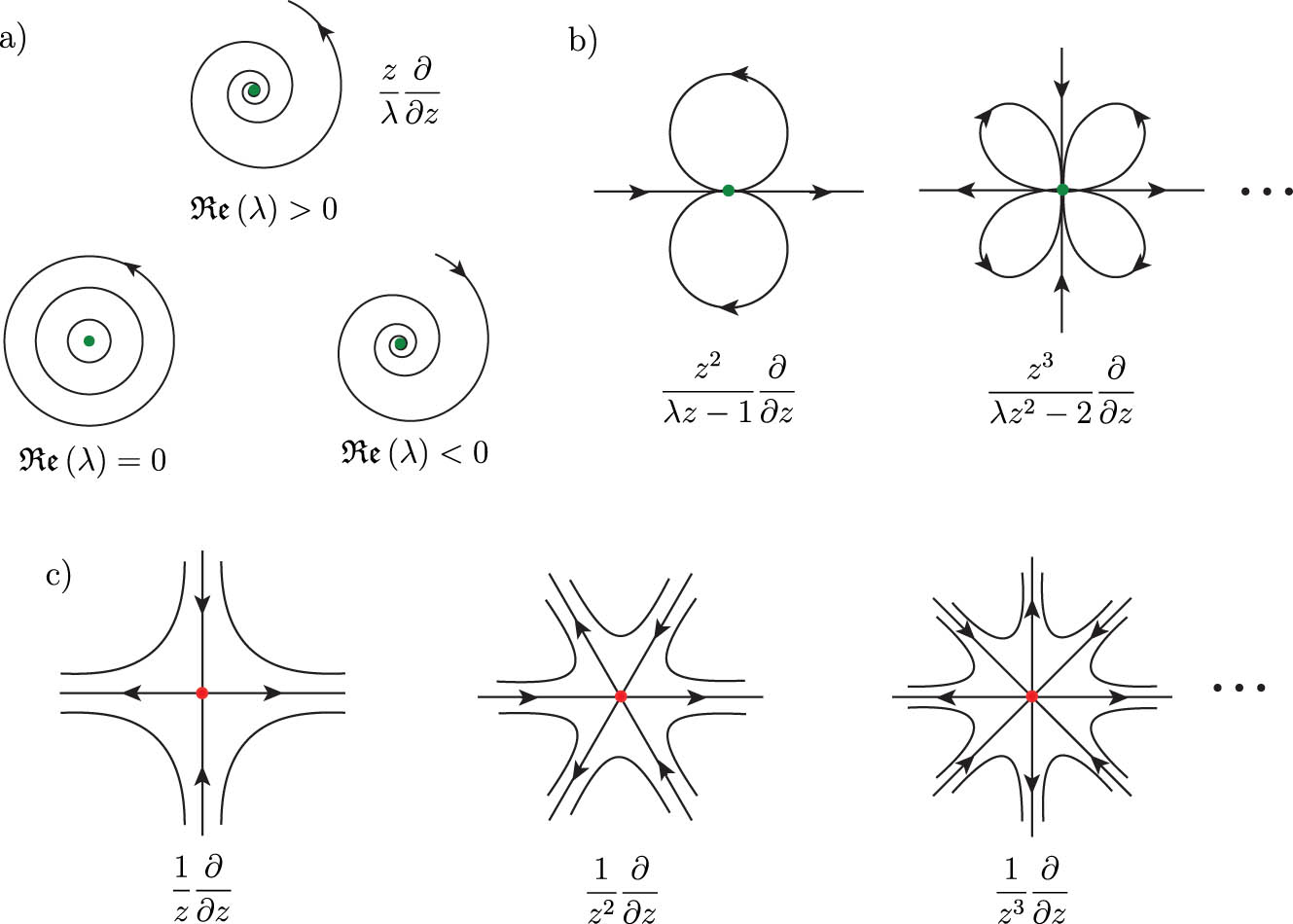
Local analytic normal forms: (a) simple zeros, (b) multiple zeros, and (c) poles of X . By simplicity, zeros and poles are at the origin.

Proposition 2.12

(Local analytic normal forms at zeros and poles of X ) Let ( ( C , z 0 ) , X ) be a germ of a singular complex analytic vector field; in each item, the corresponding assertions are equivalent.

1. X is holomorphic and non-zero at z 0 .
2. Re ( X ) is topologically equivalent to Re ∂ ∂ t .
3. Up to local biholomorphism X is ∂ ∂ z .
1. X has a zero at z 0 = q of multiplicity s ≥ 1 .
2. For multiplicity one Re ( X ) is a source, sink, or centre; for multiplicity of at least two, it admits a decomposition with 2 s − 2 ≥ 2 elliptic sectors and zero or one parabolic sectors.
3. Up to local biholomorphism, X is ( z − q ) s λ ( z − q ) s − 1 − ( s − 1 ) ∂ ∂ z , λ ∈ C .
1. X has a pole at z 0 = p of multiplicity − k ≤ − 1 .
2. Re ( X ) admits a decomposition with 2 k + 2 hyperbolic sectors.
3. Up to local biholomorphism X is 1 ( z − p ) k ∂ ∂ z .
1. X has an essential singularity at z 0 = e .
2. Re ( X ) has any other topology different from (1)–(3).

Proof

In Assertions (1)–(4), X is assumed to be holomorphic and non-zero in a punctured disk D ( z 0 , ρ ) \ { z 0 } . In (2), a parabolic sector appears if and only if Res ( ω X , z 0 ) ∈ C \ R , for further details, see [3] §5.□

3 Singularities of Ψ X ‒ 1 : ideal points of M \ S

The work of Iversen [25] originates the study of transcendental singularities of meromorphic functions, and modern expositions can be found in Bergweiler and Eremenko [8] and Eremenko [14]. In this theory, the inverse function Ψ X − 1 and the Riemann surface ℛ X play an essential role.

Remark 3.1

We consider three family functions on M :

single-valued additively automorphic singular complex analytic functions,
multivalued additively automorphic singular complex analytic functions, and
non-additively automorphic multivalued singular complex analytic functions.

The first two families are studied in Sections 3.1–3.3. The third family does not appear when we deal with vector fields, see comment on Section 7.

3.1 Single-valued additively automorphic Ψ X

In this section, we shall consider a singular complex analytic 1-form of time ω X with S R = ∅ , and hence, the domain is M \ E . In other words,

(9) Ψ X ( z ) = ∫ z o z ω X : M \ E ⟶ C ^ t , S R = ∅

is a single-valued additively automorphic singular complex analytic function, where the initial point of integration is a non-singular point z o ∈ M \ S . The integral function in equation (9) is a particular case of (5).

Definition 3.2

[8,14,25] Take a ∈ C ^ t and denote by D ( a , ρ ) ⊂ C ^ t , the disk of radius ρ > 0 (in the spherical metric) centreed at a . For every ρ > 0 , choose a component U a ( ρ ) ⊂ M of Ψ X − 1 ( D ( a , ρ ) ) in such a way that ρ 1 < ρ 2 implies U a ( ρ 1 ) ⊂ U a ( ρ 2 ) . Note that the function U a : ρ → U a ( ρ ) is completely determined by its germ at 0.

The following two possibilities below can occur for the germ of U a .

∩ ρ > 0 U a ( ρ ) = { z k } , z k ∈ M . In this case, a = Ψ X ( z k ) .
Moreover, if a ∈ C t and Ψ ′ ( z k ) ≠ 0 , or a = ∞ and z k is a simple pole of Ψ X , then z k is called an ordinary point.
On the other hand, if a ∈ C t and Ψ ′ ( z k ) = 0 , or if a = ∞ and z k is a multiple pole of Ψ X , then z k is called a critical point and a is called a critical value of Ψ X . We also say that the critical point z k lies over a. In this case, U a : ρ → U a ( ρ ) defines an algebraic singularity of Ψ X − 1 .
∩ ρ > 0 U a ( ρ ) = ∅ . We then say that our choice ρ → U a ( ρ ) defines a transcendental singularity of Ψ X − 1 and that the transcendental singularity U a lies over a.

In both cases, the open set U a ( ρ ) ⊂ M is called a neighbourhood of the singularity U a . Therefore, when ζ m ∈ M , we say that ζ m → U a if for every ρ > 0 , there exists m 0 ∈ N such that ζ m ∈ U a ( ρ ) , for m ≥ m 0 .

Remark 3.3

The germ U a of Definition 3.2 case (2) can be understood as follows.

A transcendental singularity of Ψ X − 1 , namely, U a , is equivalent to the addition of an ideal point U a to M \ E .
The addition of the ideal points { U a } , together with their corresponding neighbourhoods { U a ( ρ ) } ⊂ M , provides a Hausdorff completion/compactification of M \ E , see [2] Ch. I §6 for the general construction.
In our framework, the families of functions Ψ X ( z ) = ∫ z ( P ( ζ ) ⁄ Q ( ζ ) ) e − E ( ζ ) d ζ , in Theorem 5.1, provide prototypes of this kind of compactification, even in the multivalued case.
In what follows, we shall interchangeably refer to a transcendental singularity U a of Ψ X − 1 or an ideal point U a of M \ E .

Let z s ∈ S ⊂ M , the expression z tends to z s ∈ M makes sense. Recalling [14] p. 3, the following concept is natural.

Definition 3.4

Let U a be a transcendental singularity of Ψ X − 1 . An asymptotic value a ∈ C ^ t of Ψ X means that there exists a C 1 asymptotic path α a ( t ) : [ 0 , ∞ ) ⟶ M , α a ( 0 ) = z o ∈ M \ S , tending to z s ∈ M with well defined slope, such that
(10) a = lim t → ∞ Ψ X ( α a ( t ) ) = lim t → ∞ ∫ α a ( t ) ω X ∈ C ^ t .
We shall not distinguish between individual members α a of the class of asymptotic paths [ α a ] giving rise to the same transcendental singularity U a over a of Ψ X − 1 .
A pair ( α a , a ) is a branch point of ℛ X .

Remark 3.5

Because of Lemma 2.9.3, we will assume that the asymptotic path in Definition 3.4 ends at the singular point z s .

There is a bijective correspondence between the following:
1. classes [ α a ( t ) ] of asymptotic^[5] paths α ( t ) ,
2. asymptotic values a ∈ C ^ t counted with multiplicity,
3. transcendental singularities U a of Ψ X − 1 and
4. branch points^[6] ( α a , a ) of ℛ X .
Certainly, the notation U a can be confusing for singular values a with multiplicity two or more; in those cases, we add a subscript a σ , to distinguish them.

Definition 3.6

The singular values of Ψ X are the critical values and asymptotic values, both counted with multiplicity.

If a ∈ C ^ t is an asymptotic value of Ψ X , then there is at least one transcendental singularity U a of Ψ X − 1 over a . Certainly, there can be finite or even infinite different transcendental singularities as well as critical and ordinary points over the same singular value a .

Remark 3.7

(On the finitude of the set of asymptotic values)

The Denjoy-Carleman-Ahlfors theorem provides a sharp estimate for the number of asymptotic values when M = C ^ z . If Ψ X is an entire function with d finite asymptotic values, then the order of growth
limsup r → ∞ log M ( r ) log r = d ,
where as usual M ( r ) = max ∣ z ∣ = r ∣ Ψ X ( z ) ∣ . Compare with [39] §5.2. In fact, the order of growth is a valuable local analytic invariant, see [35] for single-valued functions. In [3], we consider this invariant for vector fields, study some families, and relate it to the number of asymptotic values.
On the other hand, there exist single-valued transcendental meromorphic functions on C z with an infinite set of asymptotic values. See Gross [16] and Eremenko [14] §4.

Definition 3.8

A transcendental singularity U a of Ψ X − 1 over a is as follows:

direct if there exists ρ > 0 such that Ψ X ( z ) ≠ a for z ∈ U a ( ρ ) , this is also true for all smaller values of ρ ,
indirect if it is not direct, i.e. for every ρ > 0 , the function Ψ X takes the value a in U a ( ρ ) , in which case the function Ψ X takes the value a infinitely often in U a ( ρ ) ,
logarithmic singularity over a if
Ψ X : U a ( ρ ) ⊂ M ⟶ D ( a , ρ ) \ { a } ⊂ C ^ t
is a universal covering for small enough ρ .

Naturally, logarithmic singularities are direct. We shall use “non-logarithmic” without the “direct” adjective when referring to direct non-logarithmic as well as indirect singularities.

Example 3.1

The simplest case of direct singularities arises from

Ψ X ( z ) = ∫ z e − ζ d ζ : C z ⟶ C t \ { 0 } .

There are logarithmic singularities over the asymptotic values 0 , ∞ ∈ C ^ t , respectively. For small enough ρ > 0 , the neighbourhoods U 0 ( ρ ) and U ∞ ( ρ ) are exponential tracts. We illustrate this in Figure 2(a).

3.2 Multivalued additively automorphic Ψ X ; the fundamental domain Λ

Consider a multivalued additively automorphic singular complex analytic function

(11) Ψ X ( z ) = ∫ z o z ω X : M \ ( E ∪ Z R ) ⟶ C ^ t , S R ≠ ∅ ,

where the initial point of integration is a non-singular point z o ∈ M \ S . The integral function in equation (11) is a particular case of (5).

One of the fundamental hurdles in studying multivalued additively automorphic functions (11) à la Iversen, Definition 3.2, is that the neighbourhoods U a ( ρ ) = Ψ X − 1 ( D ( a , ρ ) ) are not useful for distinguishing the ideal points U a . For the sake of clarity, we describe the simplest object where this occurs.

Example 3.2

(Singular points with non-zero residue) Let us consider the multivalued additively automorphic singular complex analytic function

Ψ X ( z ) = λ log ( z ) + C = λ ∫ z d ζ ζ : C ^ z \ { 0 , ∞ } ⟶ C ^ t , λ ∈ C * .

The associated ω X on C ^ z has non-zero residues at

S = Z R = { 0 , ∞ } .

On the other hand, Ψ X − 1 ( t ) = exp ( t ⁄ λ ) is an entire function that has an isolated essential singularity at ∞ ∈ C ^ t . As a consequence of Picard’s theorem applied to Ψ X − 1 , for any ρ > 0 , the neighbourhood U ∞ ( ρ ) ≐ Ψ X − 1 ( D ( ∞ , ρ ) ) is C ^ z \ { 0 , ∞ } .

In its original setting, Iversen’s theory of transcendental singularities does not make sense at 0 , ∞ ∈ C ^ z , which are poles of the associated ω X .

In other words, for every ρ > 0 , the neighbourhoods U ∞ ( ρ ) are all the same, and consequently, the ideal points U ∞ , are not well defined. As will be seen in Section 3.3, this can be explained by considering the universal cover C of C ^ z \ Z R .

The analogous behaviour of Ψ X − 1 appears for many other families of functions, e.g.

Ψ X ( z ) = ∫ z P ( ζ ) Q ( ζ ) e − E ( ζ ) d ζ ,

assuming that their 1-forms of time have non-zero residues, see Theorem 5.1.

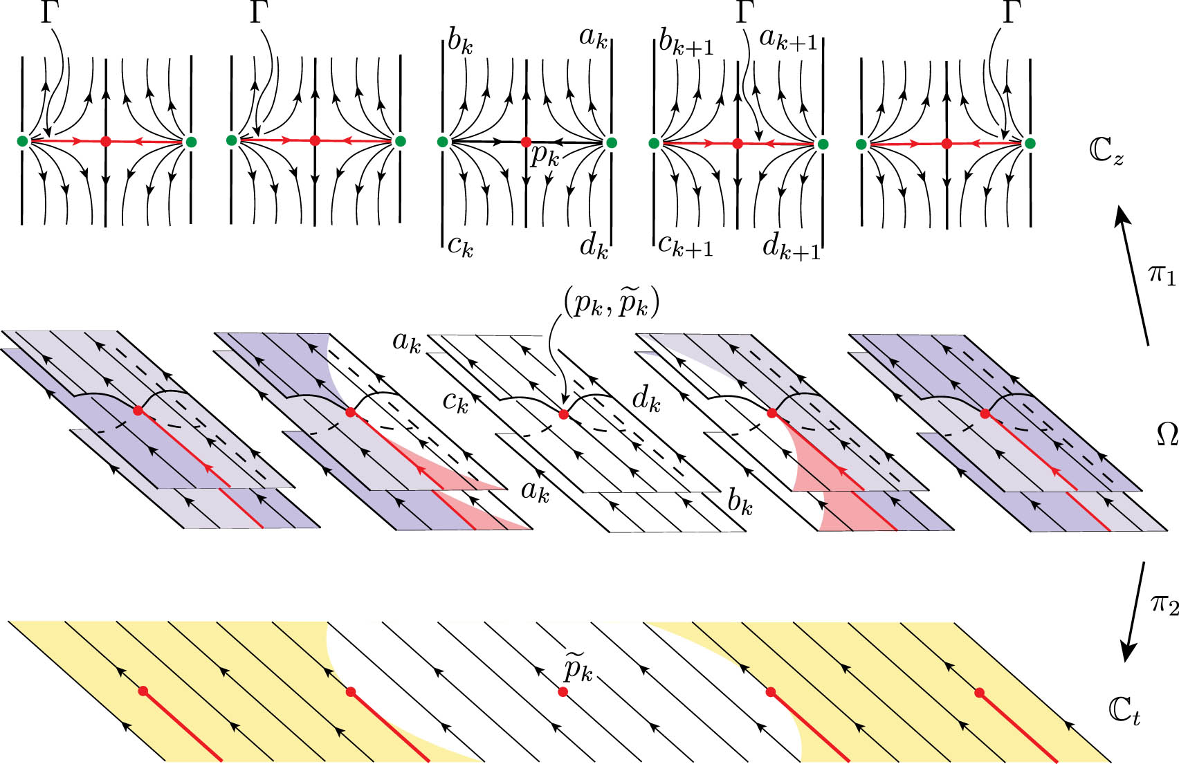
3.2.1 Construction of a fundamental domain for Ψ X

To extend Iversen’s theory of singularities of the inverse function to multivalued additively automorphic singular complex analytic functions Ψ X , note that in Diagram 8, the function Ψ X = π 1 − 1 ∘ π 2 factors through ℛ X . Very roughly speaking, for Ψ X as in equation (11), we search for a maximal univalence domain Λ for Ψ X (i.e. where Ψ X is defined and single-valued). Recalling Remark 2.4, we proceed as follows.

Let Ψ X be as in equation (11).

Assume first that M = C ^ z or the disk Δ z . (If M = C z , by adding the conformal puncture ∞ , we obtain C ^ z .) Let S R be the set of non-zero residue singular points of ω X ; assume by hypothesis that its cardinality is 2 ≤ κ ≤ ∞ (possibly infinite and numerable), i.e.
S R = { z 1 , z 2 , … , z κ } .
Assume that we have a collection of paths Γ = { γ k } k = 1 κ − 1 , where γ k is the segment of Γ between z k and z k + 1 satisfying the following:
1. Each γ k ⊂ M is a continuous simple path with extreme points in S R and avoids other singular points in S .
2. For k ≠ ℓ , the intersection γ k ∩ γ ℓ is either one point z ℓ (when ℓ = k + 1 or k − 1 ) in S R or is empty otherwise.
3. The set
  M \ Γ ¯
  is an open connected Riemann surface, where ( ) ¯ means the closure in M . Note that ω X is still a singular complex analytic 1-form on M \ Γ ¯ with singular set S \ S R ¯ .
As usual, if we cut M along γ k , we obtain two boundary paths, say γ k + and γ k − , which are considered without their extreme points z k and z k + 1 . We define
Λ 0 ≐ ( M \ Γ ¯ ) ⋃ k = 1 κ γ k + .
Simply stated, we add to the open surface M \ Γ ¯ only one boundary component γ k + for each path γ k .
In the case M ≠ C ^ z , Δ z , then M is not simply connected and we require an additional construction. Let { γ ˜ ℓ } ℓ = 1 L ⊂ M \ S be representatives of the generators of the fundamental group π 1 ( Λ 0 ) . Note that γ ˜ ℓ are simple closed paths in Λ 0 . Hence, cutting Λ 0 along the paths { γ ˜ ℓ } ℓ = 1 L and once again adding only one of their boundary components { γ ˜ ℓ + } ℓ = 1 L , we obtain
Λ = Λ 0 \ ⋃ ℓ = 1 L γ ˜ ℓ ⋃ ℓ = 1 L γ ˜ ℓ + ,
a fundamental domain for Ψ X .

Remark 3.9

Considering ω X , note that Λ ∩ S contains its
- zeros P and
- poles with residue zero Z 0 .
Furthermore, S R ¯ is in the boundary of Λ .
By construction, Λ is simply connected, has non-empty boundary, and ∫ β ω X = 0 for any closed path β in the locus, where ω X is holomorphic. The restriction of Ψ X in equations (5) and (11),
(12) Ψ X , Λ ( z ) = ∫ z o z ω X : Λ \ E ⟶ C ^ t
is a single-valued singular complex analytic function with singular set S \ S R ¯ (note that E ∪ Z R = E ∪ S R ).
In the construction of Γ , we have avoided the set of singular points, i.e. we have asked that Γ ∩ S = ∅ . This has been done for simplicity; however, note that Γ ∩ P ≠ ∅ can be allowed (this is sometimes useful), since ω X has zeros at P and Ψ X is holomorphic on P .

Definition 3.10

A fundamental region for a multivalued additively automorphic function Ψ X is

Ω = { ( z , Ψ X ( z ) ) ∣ z ∈ Λ \ E } ⊂ M × C ^ t .

Remark 3.11

Obviously, a fundamental region Ω depends on the choice of z o , { γ k } and { γ ˜ ℓ } .
The following diagram commutes(13) 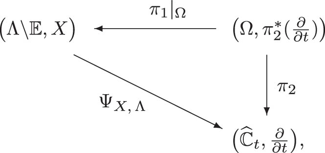where π 1 ∣ Ω and π 2 are local isometries. The fundamental domain Λ \ E and the fundamental region Ω are biholomorphic under π 1 ∣ Ω . Note that Ψ X , Λ − 1 = π 1 ∣ Ω ∘ π 2 − 1 .

Since Ψ X is single-valued on Λ , we proceed to slightly modify all the concepts in Section 3.1, by using Λ instead of M . Let α a ( t ) : [ 0 , ∞ ) ⟶ Λ be an asymptotic path, analogously as in equation (10) in Definition 3, so ( α a , a ) is the branch point in ℛ X corresponding to the path α a ( t ) → z s , and

a = lim t → ∞ Ψ X , Λ ( α ( t ) ) = lim t → ∞ ∫ α a ( t ) ω X ∈ C ^ t .

Definition 3.12

(Extension to the additively automorphic case) Let Ψ X be as in (11) and the function Ψ X , Λ , which depends on the choice of Λ be as in (12). Take a ∈ C ^ t and denote by D ( a , ρ ) ⊂ C ^ t the disk of radius ρ > 0 (in the spherical metric) centreed at a . For every ρ > 0 , first choose a connected component

V ( ( α a , a ) , ρ ) ⊂ ℛ X of π 2 − 1 ( D ( a , ρ ) ) ,

and, using Diagram 13, π 1 ∣ Ω is the restriction of π 1 to Ω , then let

U a ( ρ ) ≐ π 1 ∣ Ω ( V ( ( α a , a ) , ρ ) ) ,

in such a way that ρ 1 < ρ 2 implies U a ( ρ 1 ) ⊂ U a ( ρ 2 ) . The neighbourhoods U a ( ρ ) determine ideal points or singularities U a of Ψ X , Λ − 1 .

With the aforementioned considerations, all the definitions and results presented in Section 3.1 apply for Ψ X , Λ .

Remark 3.13

(Some consequences of the multivalued nature of Ψ X )

In our construction of the neighbourhood U a ( ρ ) , there is a choice of one connected component of π 2 − 1 ( D ( a , ρ ) ) . However, due to the choice of Γ , the projection U a ( ρ ) = π 1 ∣ Ω ( V ( ( α a , a ) , ρ ) ) can have an arbitrary number of connected components. For instance, in Examples 5.2 and 6.2 (Figures 6 and 7(a)), if the paths γ k ⊂ Γ are chosen to lie on the real axis, then at least one of the neighbourhoods U a ( ρ ) of the transcendental singularities corresponding to the essential singularity would have two connected components.
Note that, when Z R ≠ ∅ , a new type of transcendental singularity of Ψ X , Λ − 1 appears: ideal points U ∞ arising from the non-zero residue poles of ω X , see example below.

Figure 6

Let X ( z ) = z e z ∂ ∂ z , the singularities with non-zero residue are S = S R = { 0 , ∞ } . (a) The essential singularity at ∞ is represented by a small red circle. Here, Γ ⊂ C ^ z (in red) is a path from 0 to ∞ . (b) The flat metric ( C ^ z , g X ) is obtained from an infinite number of Reeb components as in e z ∂ ∂ z and a cylinder. (c) The Riemann surface ℛ X and a fundamental region Ω in the universal cover of C ^ z \ S are sketched. Three singularities U a j of Ψ X , Λ ‒ 1 whose neighbourhoods are hyperbolic and elliptic tracts (coloured green and blue, respectively), and a ⋆ -transcendental singularity coloured pink, arising from the source at z = 0 . The colouring scheme is applied both in Λ and Ω .

The following definitions are natural.

Definition 3.14

Assume that there exists an asymptotic path α ( t ) in Λ tending to a singularity z s ∈ S of ω X with asymptotic value a . The respective U a is as follows:

An essential transcendental singularity of Ψ X , Λ − 1 , when z s ∈ E .
1. A zero residue essential transcendental singularity of Ψ X , Λ − 1 , when z s ∈ E 0 .
A non-zero residue transcendental singularity of Ψ X , Λ − 1 , when z s ∈ S R = Z R ∪ E R .
1. A ⋆ -transcendental singularity of Ψ X , Λ − 1 , when z s ∈ Z R .
2. A non-zero residue essential transcendental singularity of Ψ X , Λ − 1 , when z s ∈ E R .

Example 3.3

(Example 3.2 revisited) Let

(14) Ψ X ( z ) = λ log ( z ) + 1 z s − 1 , on M = C ^ z , s ≥ 1 , λ ∈ C *

be a multivalued additively automorphic function. Let us consider Λ = C ^ z \ ( R + ∪ { 0 , ∞ } ) . The fundamental region is

Ω = z , ∫ 1 z ω X = z , λ log ( z ) + 1 z s − 1 ⊂ C ^ z × C ^ t .

Note that Ψ X is the integral of the normal form of ω X having a pole of multiplicity s ≥ 1 at z s = 0 , with non-zero residue. Thus, for all paths α ( t ) → 0 in Λ , the asymptotic value of Ψ X , Λ is ∞ and the corresponding transcendental singularity U ∞ of Ψ X , Λ − 1 lies over ∞ . The neighbourhoods U ∞ ( ρ ) ⊂ Λ contain D ( 0 , r ( ρ , λ ) ) ∩ Λ , for suitable radius r ( ρ , λ ) , which tend to 0 when ρ → 0 ; hence, Definition 3.12 is satisfied. According to Definitions 3.8 and 3.14, it is a direct singularity, which is not logarithmic; thus, U ∞ is a ⋆ -transcendental singularity of Ψ X , Λ − 1 . Figure 8 illustrates the generic behaviour of Ψ X , where the parabolic sector depending on λ appears; for an accurate explanation, see [3] §5.

Note that for the singular point z s = ∞ , the study is completely analogous.

$Figure 7 We regard the vector field X ( z ) = z ( z ‒ 1 ) e ‒ z ∂ ∂ z X\left(z)=z\left(z‒1){{\rm{e}}}^{‒z}\frac{\partial }{\partial z} , Example 6.2. (a) To better visualize the behaviour, we show the pullback vector field Y ( w ) = ( T * X ) ( w ) Y\left(w)=\left({T}^{* }X)\left(w) , with T ( w ) = w ⁄ ( ‒ w + 1 ) T\left(w)=w/\left(‒w+1) ; the blue and green points correspond to the zeros of Y Y , and the red point is the essential singularity of Y Y . The red arcs of a circle correspond to the inverse images of Γ \Gamma . The hyperbolic and elliptic tracts are shaded green and blue, respectively, while the ⋆ \star -transcendental singularities corresponding to the zeros are pink. (b) Shows the universal cover M ≅ Δ {\mathfrak{M}}\cong \Delta and some copies of the fundamental domain Λ \Lambda . Note that the ideal points of Ψ X ˜ ‒ 1 {\widetilde{{\Psi }_{X}}}^{‒1} form a countable dense set on the boundary ∂ Δ \partial \Delta of the disk Δ \Delta . Each neighbourhood of these ideal points is composed by an infinite number of angular sectors with angle 0. Each angular sector is a tract of the ideal point of Ψ X , Λ ‒ 1 {\Psi }_{X,\Lambda }^{‒1} with the same behaviour. In this example: hyperbolic tracts (green), elliptic tracts (blue), and parabolic sectors (pink).$

Figure 7

We regard the vector field X ( z ) = z ( z ‒ 1 ) e ‒ z ∂ ∂ z , Example 6.2. (a) To better visualize the behaviour, we show the pullback vector field Y ( w ) = ( T * X ) ( w ) , with T ( w ) = w ⁄ ( ‒ w + 1 ) ; the blue and green points correspond to the zeros of Y , and the red point is the essential singularity of Y . The red arcs of a circle correspond to the inverse images of Γ . The hyperbolic and elliptic tracts are shaded green and blue, respectively, while the ⋆ -transcendental singularities corresponding to the zeros are pink. (b) Shows the universal cover M ≅ Δ and some copies of the fundamental domain Λ . Note that the ideal points of Ψ X ˜ ‒ 1 form a countable dense set on the boundary ∂ Δ of the disk Δ . Each neighbourhood of these ideal points is composed by an infinite number of angular sectors with angle 0. Each angular sector is a tract of the ideal point of Ψ X , Λ ‒ 1 with the same behaviour. In this example: hyperbolic tracts (green), elliptic tracts (blue), and parabolic sectors (pink).

We obtain the following normal forms summary for poles and zeros of ω X :

Singularity of Ψ X − 1	Ψ X ( z )	ω X ( z )	X ( z )	Parameters
Algebraic for λ = 0				s ≥ 1 ,
⋆ -transcendental for λ ≠ 0	λ log ( z ) + 1 z s − 1	λ z − s − 1 z s d z	z s λ z s − 1 − ( s − 1 ) ∂ ∂ z	residue λ ∈ C
Algebraic	z k + 1 k + 1	z k d z	1 z k ∂ ∂ z	k ≥ 1

Remark 3.15

The transcendental singularities of Ψ X − 1 that appear in the classical theory of single-valued functions Ψ X , as in Definition 3.2, are all zero residue essential transcendental singularities, as in Definition 3.14.1.i.
In Definition 3.14.2.i, since z s ∈ Z R , the asymptotic value is necessarily a = ∞ ∈ C ^ t .
Note that non-zero residue essential transcendental singularities, Definition 3.14.2.ii, are also essential transcendental singularities, Definition 3.14.1.

An accurate description of the singular values for Ψ X , Λ is required. In Definition 3.12, there is a choice of fundamental domain Λ , equivalently of a fundamental region Ω ⊂ ℛ X . This actually makes a difference on what is considered a singular value of Ψ X , Λ .

Let Ψ X be a multivalued additively automorphic singular complex analytic function, equation (11), and assume that a ∈ C ^ t is a singular value of Ψ X , Λ with asymptotic path α a ( t ) ⊂ Λ .

Now, consider a path or class ϱ ∈ π 1 ( M \ S R ¯ ) , that starts at the non-singular point z o ∈ M \ S , defining

Ξ ϱ ≐ ∫ ϱ ω X .

Then

lim t → ∞ ∫ ϱ ω X + ∫ α a ( t ) ω X = Ξ ϱ + a .

In other words, the linear combinations Ξ ϱ ∈ C * of residues and periods of ω X determine an infinite collection { a + Ξ ϱ } ⊂ C consisting of:

a singular value a ∈ C ^ t of Ψ X , Λ and
an infinite number of fake singular values, one for each possible non-zero linear combination Ξ ϱ .

Of course, the only true singular value of Ψ X , Λ is a , since the paths ϱ concatenated with α a do not lie in Λ unless ϱ is homotopic to the identity.

Proposition 3.16

(Configurations of singular values amongst fundamental regions) Let Ψ X : M \ ( E ∪ Z R ) ⟶ C ^ t be a multivalued additively automorphic singular complex analytic function as in (11).

Given any two fundamental regions Ω 1 and Ω 2 , the singular values { a j } and { a ˜ j } of Ψ X , Λ 1 and Ψ X , Λ 2 , respectively, satisfy
a j = a ˜ j + Ξ ϱ , for j = 1 , … , m or i n f i n i t e a n d n u m e r a b l e { j } ,
where Ξ ϱ ∈ C is a fixed linear combination of the residues and periods of ω X , which depends on the choice of the two fundamental regions Ω 1 , Ω 2 and on the initial point of integration z o for Ψ X .
The qualitative behaviour of the ideal points U a associated with Ψ X , Λ 1 and U a + Ξ ϱ associated with Ψ X , Λ 2 is independent of the choice of fundamental regions Ω 1 or Ω 2 .

Proof

For (1), given two different fundamental regions, say Ω 1 and Ω 2 , the corresponding Λ 1 = π 1 ( Ω 1 ) and Λ 2 = π 1 ( Ω 2 ) are simply connected subsets of the universal cover. There exists an element ϱ of the fundamental group π 1 ( M \ S R ¯ ) such that Λ 2 = ϱ ( Λ 1 ) as a cover transformation. Therefore, given a singular value a ∈ C ^ t of Ψ X , Λ 1 , the value a + Ξ ϱ ∈ C ^ t is the corresponding singular value of Ψ X , Λ 2 .

For (2), note that Ψ X , Λ 1 and Ψ X , Λ 2 differ only by the value Ξ ϱ ∈ C t . However, since Ω 1 and Ω 2 are copies of each other (up to cutting and pasting and using the flat metric g X on ℛ X arising from π 2 * ( ∂ ∂ t ) ). Then, the branch points associated with U a in ( Ω 1 , π 2 * ( ∂ ∂ t ) ) and U a + Ξ ϱ in ( Ω 2 , π 2 * ( ∂ ∂ t ) ) are related by the cover transformation ϱ . Hence, the ideal points arising from either Λ 1 or Λ 2 are qualitatively the same.□

3.3 A model for ℛ X ; the universal cover of M \ S R ¯

Once again, we consider a multivalued additively automorphic singular complex analytic function as in (11), namely,

Ψ X ( z ) = ∫ z o z ω X : M \ ( E ∪ Z R ) ⟶ C ^ t , S R ≠ ∅ ,

where the initial point of integration is a non-singular point z o ∈ M \ S . Let

π : M ⟶ M \ S R ¯

be the universal cover of M \ S R ¯ . The analytic extension of Ψ X to M , namely,

Ψ X ˜ ( z ) = ∫ z π * ω X : M \ π − 1 ( E 0 ) ⟶ C ^ ,

is a single-valued additively automorphic singular complex analytic function, and thus, Section 3.1 applies. As a mater of record,

X ˜ = π * X on M

denotes the singular complex analytic vector field associated with Ψ X ˜ . Moreover, by Lemma 2.9.2, we have that

ℛ X = ∪ ϱ Ω ϱ ≅ M , ϱ ∈ π 1 ( M \ S R ¯ ) .

In fact, the surface ℛ X ⊂ M × C ^ t in (6) can be reconstructed by using copies of the fundamental region Ω by the analytical continuation of Ψ X across the γ k as in the construction of Λ . Note that the Ω ϱ are isometric copies of Ω , using the flat metric g X on ℛ X arising from π 2 * ( ∂ ∂ t ) .

Remark 3.17

Even though in M the corresponding 1-form of time ω ˜ X ≐ d Ψ X ˜ always has zero residues, we shall still add the adjective non-zero residue when naming those transcendental singularities U ˜ a of Ψ X ˜ − 1 whose corresponding singularity U a ≐ π ( U ˜ a ) is a non-zero residue transcendental singularity of Ψ X , Λ − 1 . See Definition 3.14.2.
Assuming that S R ¯ ≠ ∅ , by simple inspection, we obtain that M is biholomorphic to Δ or C , the case C ^ does not appear.

A direct application of Proposition 3.16 yields the following result.

Corollary 3.18

Let Ψ X : M \ ( E ∪ Z R ) ⟶ C ^ t be a multivalued additively automorphic singular complex analytic function, as in (11), with fundamental domain Λ , and let Ψ X ˜ : M \ π − 1 ( E 0 ) ⟶ C ^ be its extension to the universal cover M .

For each singular value a ∈ C ^ t of Ψ X , Λ , there are an infinite number of singular values { a + Ξ ϱ ∣ ϱ ∈ π 1 ( M \ S R ¯ ) } ⊂ C t of Ψ X ˜ . In case that a = ∞ , the singular value ∞ of Ψ X ˜ has infinite multiplicity.
The function Ψ X ˜ has an infinite number of ideal points U ˜ a + Ξ ϱ , each of which has the same qualitative behaviour, on each copy of Λ , as that of the ideal point U a of Ψ X , Λ .
When M is compact and M is biholomorphic to Δ , the non-zero residue transcendental singularities of Ψ X ˜ , say { U ˜ a } , are a dense subset of ∂ Δ .
When M is biholomorphic to C , consider its compactification C ^ z .
1. If S = S R = Z R , then ∞ ∈ C ^ z is a simple pole of Ψ X ˜ .
2. If S = S R ≠ Z R , then ∞ is an isolated essential singularity of Ψ X ˜ .
3. Otherwise, ∞ is an non-isolated essential singularity of Ψ X ˜ .

Proof

Assertion (3) is true by simple inspection.

For assertion (4), assume that Ψ X : C ^ z ⟶ C ^ t and S R = { 0 , ∞ } , and thus, the lift to the universal cover is

Ψ X ˜ : C z ⟶ C ^ t ,

which has a singularity at ∞ ∈ C ^ z .

Case (i), where S = Z R is equal to two simple poles of ω X at 0 , ∞ , determines a simple pole of Ψ X ˜ at ∞ , recalling the normal form of ω X in Proposition 5.

By an analogous argument in case (ii), since S = S R ≠ Z R , it follows that Ψ X ˜ has an isolated singularity at ∞ . Once again, by Proposition 5 it is an essential singularity of Ψ X ˜ .

For case (iii), if S R is equal to two points 0 , ∞ , and S R ≠ S , then the singularity of Ψ X ˜ at ∞ has an accumulation of the zero residue singularities, in complete detail, points in Z 0 ∪ P .□

The non-compact case for M in assertion (3) of Corollary 3.18 is left to the reader.

3.4 Equivalence relation on the singularities of Ψ X , Λ ‒ 1

Because of the biholomorphism between ℛ X and the universal cover M of M \ S R ¯ , and Proposition 3.16.2, it is natural to define an equivalence relation for different choices of Λ .

Definition 3.19

Consider two singularities U a ⊂ Λ 1 of Ψ X , Λ 1 − 1 over a ∈ C ^ t , and U a ˜ ⊂ Λ 2 of Ψ X , Λ 2 − 1 over a ˜ ∈ C ^ t . They are in the same equivalence class [ [ U a ] ] if there exists a cover transformation ϱ ∈ π 1 ( M \ S R ¯ ) such that the following occurs:

Ω 2 = ϱ ( Ω 1 ) ⊂ ℛ X ,
a = a ˜ + Ξ ϱ , where Ξ ϱ = ∫ ϱ ω X ,
for each ρ > 0 , there exist ρ 1 , ρ 2 > 0 such that
ϱ ( π 1 − 1 ( U a ( ρ 1 ) ) ) ⊂ π 1 − 1 ( U a ˜ ( ρ ) ) ⊂ Ω 2 ⊂ ℛ X
and
ϱ − 1 ( π 1 − 1 ( U a ˜ ( ρ 2 ) ) ) ⊂ π 1 − 1 ( U a ( ρ ) ) ⊂ Ω 1 ⊂ ℛ X .

There exists an equivalence class [ ⋅ ] of singular values induced by the equivalence class [ [ ⋅ ] ] .

We shall say [ [ U a ] ] is a singularity class of Ψ X − 1 over the singular value class [ a ] .

The equivalence relation is well defined; we leave the proof for the interested reader.

Remark 3.20

Clearly, condition (b) in Definition 3.19 is necessary but not sufficient for the equivalence relation on the singular values.
A convenient abuse of notation is to say
“the singularity U a of Ψ X − 1 over the singular value a ,”
when in reality, we should say
“ the singularity class [ [ U a ] ] of Ψ X − 1 over the singular value class [ a ] .”

4 Singularities of Ψ X ‒ 1 from the perspective of vector fields

Because of the correspondence between singular complex analytic vector fields X and additively automorphic singular complex analytic functions Ψ X , given by Proposition 2.6; the study of the singularities of Ψ X − 1 , both in the single-valued case and in the multivalued additively automorphic case, benefits from the perspective of vector fields.

Example 4.1

(Example 3.1 revisited) The distinguished parameter

Ψ X ( z ) = ∫ z e − ζ d ζ : C z ⟶ C t \ { 0 } ,

with two logarithmic singularities over the asymptotic values 0 and ∞ , has

X ( z ) = e z ∂ ∂ z

as its associated vector field. By considering the phase portrait of the associated vector field, the exponential tracts

U 0 ( ρ ) = { Re ( z ) > log ( 1 ⁄ ∣ ρ ∣ ) } over the asymptotic value 0, and

U ∞ ( ρ ) = { Re ( z ) < log ( 1 ⁄ ∣ ρ ∣ ) } over the asymptotic value ∞

can be clearly distinguished (Figures 1 and 2(a)).

As an advantage of the existence of a vector field X associated with a function Ψ X , we can refine exponential tracts.

Definition 4.1

The pairs
U H = { Re ( z ) > 0 } , e z ∂ ∂ z , U E = { Re ( z ) < 0 } , e z ∂ ∂ z
are the hyperbolic tract over 0 and elliptic tract over ∞ of X ( z ) = e z ∂ ∂ z , respectively (Figure 1).
The pair ( U a ( ρ ) , X ) is a hyperbolic tract over the asymptotic value a of X, or elliptic tract over the asymptotic value a = ∞ of X , if there is a biholomorphism ϒ : ( U a ( ρ ) , X ) ⊂ M ⟶ U H , or to U E , respectively.

Certainly, the notion of biholomorphism is rigid. It is suitable for our present work since we gain flexibility of this notion by applying it to open Jordan domains of ( M , X ) and under variations of the radius ρ .

Let us recall the following theorem, cited in Section 1 in a brief version, due to Nevanlinna, that applies to single-valued functions.

Theorem

(Nevanlinna’s isolated singular values, [35] Ch. XI §1.3, [46] Theorem 6.2.2) Let Ψ X : C z ⟶ C ^ t be a single-valued meromorphic function, and let a be an isolated singular value for Ψ X . If U a is a singularity of Ψ X − 1 over a , then U a is algebraic or logarithmic.

As an immediate consequence, direct non-logarithmic and indirect singularities of (single-valued) Ψ X − 1 over a imply that the singular value a is non-isolated, i.e. a is an accumulation point of singular values of Ψ X . There are, however, logarithmic singularities of Ψ X − 1 over non-isolated asymptotic values a ; see, for instance, Example 5.7 and its corresponding Figure 9. However, for multivalued additively automorphic functions, Ψ X we also have to consider the non-zero residue transcendental singularities of Ψ X − 1 , see Definition 3.14.2. As seen in Remark 3.15.2, the ⋆ -transcendental singularities of Ψ X , Λ − 1 are not algebraic or logarithmic even though the asymptotic value ∞ is isolated (in fact it is a direct non-logarithmic singularity over the isolated singular value ∞ ∈ C ^ t ).

$Figure 8 A pole of ω X = ( ( λ ⁄ z ) ‒ ( s ‒ 1 ) ⁄ z s ) d z {\omega }_{X}=\left(\left(\lambda /z)‒\left(s‒1)/{z}^{s}){\rm{d}}z of order s s at least 2, and non-zero residue λ \lambda . The associated vector field X X has 2 s ‒ 2 ≥ 2 2s‒2\ge 2 elliptic sectors and one parabolic sector. The behaviour of the function Ψ X {\Psi }_{X} , equation (14), is called an s-fold unbranched holomorphic log-covering. The parabolic sector (and its corresponding images in Ω \Omega and C ^ t {\widehat{{\mathbb{C}}}}_{t} ) has been coloured pink for clarity. This illustrates a ⋆ \star -transcendental singularity of Ψ X , Λ ‒ 1 {\Psi }_{X,\Lambda }^{‒1} .$

Figure 8

A pole of ω X = ( ( λ ⁄ z ) ‒ ( s ‒ 1 ) ⁄ z s ) d z of order s at least 2, and non-zero residue λ . The associated vector field X has 2 s ‒ 2 ≥ 2 elliptic sectors and one parabolic sector. The behaviour of the function Ψ X , equation (14), is called an s-fold unbranched holomorphic log-covering. The parabolic sector (and its corresponding images in Ω and C ^ t ) has been coloured pink for clarity. This illustrates a ⋆ -transcendental singularity of Ψ X , Λ ‒ 1 .

The aforementioned discussion shows that when working with multivalued additively automorphic singular complex analytic functions, it is not enough to just consider the singular values of the ideal points U a ; one must also examine the neighbourhoods U a ( ρ ) . For this, we introduce the following concept, understood as in Remark 3.20.2, i.e. with a choice of a fundamental domain Λ .

Definition 4.2

For Ψ X , an additively automorphic singular complex analytic function, let U a and U b be singularities of Ψ X − 1 over the singular values a and b , respectively. A singularity U a is separate if there exists ρ > 0 such that

U a ( ρ ) ∩ U b ( ρ ) = ∅ , for all U b ≠ U a .

In the aforementioned definition the case a = b is possible, see Example 4.2. In words, the ideal point U a is separate if for small enough ρ > 0 the neighbourhood U a ( ρ ) does not intersect any neighbourhood of another ideal point. Similarly, an ideal point is non-separate if and only if any neighbourhood U a ( ρ ) always intersects a neighbourhood of another ideal point.

Example 4.2

Separate singularities, case a = b . Consider
X ( z ) = e z 3 z 2 ∂ ∂ z .

The corresponding Ψ X − 1 has six logarithmic singularities arising from the essential singularity of X at ∞ ∈ C ^ z and an algebraic singularity arising from the pole of X at the origin. All the singularities of Ψ X − 1 are separate. The asymptotic values are

a 1 = a 2 = a 3 = 0 , and ∞ 1 = ∞ 2 = ∞ 3 = ∞ ,

i.e. there are two asymptotic values, each of multiplicity 3. As can be seen in Figure 2(b), there are six singularities of Ψ X − 1 , corresponding to three hyperbolic tracts over 0 and three elliptic tracts over ∞ . Full details appear in Example 4.2 of [5].

Thus, the singular values a and b can be the same and yet U a and U b can be different singularities of Ψ X − 1 .

(2) Non-separate singularities, case a ≠ b . In Example 5.7,

Ψ X ( z ) = e sin ( z ) − z ,

is considered. Among other things, it is shown that for any given ρ > 0 , each neighbourhood U ∞ , − ( ρ ) and U 0 , + ( ρ ) , with asymptotic values ∞ and 0, respectively, contains:

an infinite number of neighbourhoods U a k ± ( ρ ) , with asymptotic value 0 or ∞ , for k odd or even, respectively,
an infinite number of critical points.

Thus, both U ∞ , − ( ρ ) and U 0 , + ( ρ ) are non-separate, Figure 9 illustrates this fact.

Remark 4.3

The notion of separate is of a topological nature. Thus, even when dealing with multivalued additively automorphic singular analytic functions Ψ X , for small enough ρ > 0 , the neighbourhoods { U a ( ρ ) } are well defined. One just needs to recall that as soon as a choice of fundamental domain Λ has been made, all happens inside the chosen Λ .

With the notion of separate singularity of Ψ X − 1 , we can improve Nevanlinna’s isolated singular values theorem.

Theorem 4.4

(Separate singularities) Let Ψ X : M ⟶ C ^ t be a additively automorphic singular complex analytic function, as in (5). A singularity U a of Ψ X − 1 is separate if and only if U a is one of the following:

algebraic,
⋆ -transcendental,
logarithmic.

Proof

( ⇐ ) For cases (1) and (3), note that

Ψ X , Λ : U a ( ρ ) ⟶ D ( a , ρ ) \ { a }

is an unbranched holomorphic covering for sufficiently small ρ > 0 . In case (1), the covering is of finite degree, and in case (2), it is the universal covering, in accordance with Definition 3.8. In either case, U a is separate.

For case (2), recall that equation (14) provides a local normal form as follows:

Ψ X , Λ ( z ) = λ log ( z ) + 1 ⁄ z s − 1 , for s ≥ 1 .

Moreover, the asymptotic value is a = ∞ and the neighbourhoods of U ∞ are (up to biholomorphism) of the form U ∞ ( ρ ) ≅ ( D ( 0 , R ) \ [ 0 , R ] ) ∪ [ 0 , R ] + , recalling the construction of Λ in Section 3.2.1.3. In fact,

Ψ X , Λ : U ∞ ( ρ ) ≅ ( D ( 0 , R ) \ [ 0 , R ] ) ∪ [ 0 , R ] + ⟶ D ( ∞ , ρ ) \ { ∞ } z ⟼ λ log ( z ) + 1 ⁄ z s − 1

topologically is an s -fold unbranched holomorphic log-covering i.e. 2 s − 2 elliptic sectors followed by a parabolic sector determining λ (Figure 8). Clearly, U a is separate.

( ⇒ ) Now, we assume that U a is separate. Thus, given U b ≠ U a , there exists ρ > 0 such that U a ( ρ ) ∩ U b ( ρ ) = ∅ in Λ . In particular, this implies that U a ( ρ ) does not contain any singular points other than z s = lim t → ∞ α a ( t ) , where α a is the asymptotic path corresponding to U a .□

Recalling Definition 3.12, Ψ X , Λ = π 2 ∘ π 1 − 1 ∣ Λ . In fact,

(15) π 2 : V ( ( α a , a ) , ρ ) ⟶ D ( a , ρ ) \ { a }

is an unbranched holomorphic covering, and

π 1 ∣ Ω : Ω ⟶ Λ \ E 0 ⊂ M

is a biholomorphism. It follows that for any neighbourhood U a ( ρ ) ⊂ Λ of a singularity U a of Ψ X − 1 , one has the diagram

(16)

where V ( ( α a , a ) , ρ ) is the component of π 2 − 1 ( D ( a , ρ ) ) such that

U a ( ρ ) ≐ π 1 ∣ Ω ( V ( ( α a , a ) , ρ ) ) .

Thus, to specify the neighbourhood U a ( ρ ) , we first choose a connected component V ( ( α a , a ) , ρ ) ⊂ ℛ X of π 2 − 1 ( D ( a , ρ ) ) .

Since (15) is an unbranched holomorphic covering, it follows that the closure of V ( ( α a , a ) , ρ ) in ℛ X is topologically a disk or a punctured disk.

Having identified V ( ( α a , a ) , ρ ) , we now intersect with Ω . Once again, recalling the construction of Λ , particularly Γ , in Section 3.2.1.3, three cases appear:

∂ Ω ∩ V ( ( α a , a ) , ρ ) = ∅ , or
∂ Ω ∩ V ( ( α a , a ) , ρ ) = γ ^ 1 for a simple path γ ^ 1 that has as one of its extrema the branch point ( α a , a ) .
∂ Ω ∩ V ( ( α a , a ) , ρ ) = γ ^ 1 ∪ γ ^ 2 ,

for some simple paths γ ^ 1 ∪ γ ^ 2 ⊂ ℛ X that have as common extrema the branch point ( α a , a ) .

Note that π 1 ( γ ^ j ) = γ j ⊂ Γ ⊂ M .

In case (A), since π 1 ∣ Ω is a biholomorphism, it follows immediately that

Ψ X , Λ = π 2 ∘ π 1 − 1 ∣ Λ : U a ( ρ ) ⟶ D ( a , ρ ) \ { a }

is an unbranched holomorphic covering. Thus, by [46] Theorem 6.1.1, either:

(A.i) there exists a biholomorphism Φ of U a ( ρ ) onto Δ * ≐ { z ∣ 0 < ∣ z ∣ < 1 } such that Ψ X , Λ = Φ k for some natural number k , or

(A.ii) there exists a biholomorphism Φ of U a ( ρ ) onto the left half plane H − = { z ∣ Re ( z ) < 0 } such that Ψ X , Λ = exp ∘ Φ .

For (A.i), U a is algebraic and for (A.ii), U a is logarithmic.

Let us now examine cases (B) and (C). By Definition 3.2, for 0 < ρ ′ < ρ , the neighbourhoods satisfy V ( ( α a , a ) , ρ ′ ) ¯ ⊂ V ( ( α a , a ) , ρ ) , where the closure is in ℛ X .

Since (15) is an unbranched holomorphic covering, the closure of V ( ( α a , a ) , ρ ) in ℛ X is topologically a disk or a punctured disk.

Lemma 4.5

Let 0 < ρ ′ < ρ . The paths γ ^ 1 and γ ^ 2 can be deformed to γ ^ ˆ 1 and γ ^ ˆ 2 , within V ( ( α a , a ) , ρ ) so that:

γ ^ ˆ 1 and γ ^ ˆ 2 do not intersect V ( ( α a , a ) , ρ ′ ) , when V ( ( α a , a ) , ρ ) is topologically a disk,
γ ^ ˆ 1 and γ ^ ˆ 2 coincide inside V ( ( α a , a ) , ρ ′ ) , when V ( ( α a , a ) , ρ ) is topologically a punctured disk.

Figure 10 illustrates the lemma. Note that the paths γ ^ 1 and γ ^ 2 do not change outside of V ( ( α a , a ) , ρ ) , hence do not affect other singularities of Ψ X , Λ − 1 .

$Figure 9 Example 5.7, function Ψ X ( z ) = e sin ( z ) ‒ z {\Psi }_{X}\left(z)={{\rm{e}}}^{\sin \left(z)‒z} and phase portrait of the corresponding vector field X ( z ) = e sin ( z ) ‒ z cos ( z ) ‒ 1 ∂ ∂ z X\left(z)=\frac{{{\rm{e}}}^{\sin \left(z)‒z}}{\cos \left(z)‒1}\frac{\partial }{\partial z} . The neighbourhoods U ∞ , ‒ ( ρ ) {U}_{\infty ,‒}\left(\rho ) and U 0 , + ( ρ ) {U}_{0,+}\left(\rho ) of the non-separate singularities are coloured purple and orange, respectively.$

Figure 9

Example 5.7, function Ψ X ( z ) = e sin ( z ) ‒ z and phase portrait of the corresponding vector field X ( z ) = e sin ( z ) ‒ z cos ( z ) ‒ 1 ∂ ∂ z . The neighbourhoods U ∞ , ‒ ( ρ ) and U 0 , + ( ρ ) of the non-separate singularities are coloured purple and orange, respectively.

Proof

Follows immediately from the fact that U a is separate, and hence, we can deform γ 1 and γ 2 in the open set U a ( ρ ) \ U a ( ρ ′ ) ¯ , leaving the extrema at ∂ U a ( ρ ) and the branch point ( α a , a ) fixed.□

Case (i) tells us that ∂ Ω ∩ V ( ( α a , a ) , ρ ′ ) = ∅ , and we have reduced to case (A) above, so U a is an algebraic or logarithmic singularity of Ψ X , Λ − 1 .

For case (ii), up to biholomorphism

V ( ( α a , a ) , ρ ′ ) ∩ Ω = ( D ( 0 , R ) \ [ 0 , R ] ) ∪ [ 0 , R ] + ⊂ ℛ X ,

note that [ 0 , R ] projects by π 1 to a trajectory of Re ( X ) . By simple inspection, we can recognize that Figure 8 describes Ψ X . Thus, the singularity U a is a ⋆ -transcendental singularity of Ψ X , Λ − 1 . This completes the proof of Theorem 4.4.□

A list of the simplest singular behaviours is provided by the theorem below.

Theorem 4.6

(Topological behaviour of Re ( X ) and the singularities of Ψ X − 1 ) Let X be a singular complex analytic vector field and Ψ X the corresponding additively automorphic singular complex analytic function, as in (5). Considering the phase portrait of Re ( X ) on the neighbourhood U a ( ρ ) for small enough ρ > 0 , the name of the singularity of X, the type of singularity of Ψ X − 1 , and the residue of the 1-form of time ω X at z s ∈ S with asymptotic value a ∈ C ^ t as in Definition 3.4, a partial correspondence is

( U a ( ρ ) , Re ( X ) ) consists of	Name of the singularity of X	Type of the singularity of Ψ X − 1	Value of Res ( ω X , z s )
( 2 k + 2 ) hyperbolic sectors	pole p ∈ P of multiplicity − k ≤ − 1	algebraic singularity U a over a ∈ C t	0
( 2 s − 2 ) elliptic sectors	q ∈ Z 0	algebraic singularity U ∞ over ∞	0
and parabolic sectors	zero q ∈ Z of multiplicity s ≥ 2
	q ∈ Z R	⋆ -transcendental singularity U ∞ over ∞	C *
Source, sink or centre	Simple zero q ∈ Z R	⋆ -transcendental singularity U ∞ over ∞	C *
Hyperbolic tract	Isolated essential singularity e ∈ E	Logarithmic transcendental singularity U a over a ∈ C t	C
Elliptic tract	isolated essential singularity e ∈ E	Logarithmic transcendental singularity U ∞ over ∞	C
?	Essential singularity e ∈ E	Non separate essential transcendental singularity U a over a ∈ C ^ t	C

□

Remark 4.7

The aforementioned result emphasizes the dichotomy between finite and infinite singular values of Ψ X .
A singular value a ∈ C ^ t can admit several ideal points { U a } over it.
In the table of Theorem 4.6, the question mark in the last row means that many other topologies occur. For instance, the last row contains direct and non-direct singularities.

By Lemma 2.9.3, each asymptotic path of Ψ X can be realized as a trajectory z ( t ) of Re ( e i θ X ) with α or ω -limit z s , for some θ , the converse is obvious.

Definition 4.8

A singularity z s ∈ M of X is reachable when there exists an asymptotic path of Ψ X with limit z s .

Example 4.3

(A non-reachable singularity) Note that, not all singularities of X have an associated singularity of Ψ X − 1 . In our framework, the choice of a singular point z s ∈ S of X does not imply the existence of an asymptotic path and its asymptotic value. For instance, consider the singular complex analytic vector field

X ( z ) = cosh z cos z ∂ ∂ z .

It has simple zeros at i ( 4 k ± 1 ) π 2 and simple poles at ( 4 k ± 1 ) π 2 , for k ∈ Z . Thus, z s = ∞ ∈ E n R is an accumulation point of Z R ∪ P (Figure 11). However, since there is no asymptotic path tending to z s = ∞ , there is no singularity of Ψ X − 1 associated with z s = ∞ . Elliptic functions ℘ ( z ) in C z provide analogous examples.

$Figure 10 Deformation of the paths γ ^ 1 {\widehat{\gamma }}_{1} and γ ^ 2 {\widehat{\gamma }}_{2} inside the conformal disk V ( ( α a , a ) , ρ ) ⊂ ℛ X V(\left({\alpha }_{a},a),\rho )\subset {{\mathcal{ {\mathcal R} }}}_{X} , as in Lemma 4.5. The red circle represents the branch point ( α a , a ) \left({\alpha }_{a},a) . (a) and (b) in the figure refer to cases (a) and (b) of Lemma 4.5.$

Figure 10

Deformation of the paths γ ^ 1 and γ ^ 2 inside the conformal disk V ( ( α a , a ) , ρ ) ⊂ ℛ X , as in Lemma 4.5. The red circle represents the branch point ( α a , a ) . (a) and (b) in the figure refer to cases (a) and (b) of Lemma 4.5.

Theorem 4.9

(Ideal points in terms of singularities of X ) Let Ψ X be an additively automorphic singular complex analytic function, as in (5), and X its corresponding singular complex analytic vector field. A reachable singularity z s ∈ S of X determines at least one singularity of Ψ X − 1 .

If the singularity z s ∈ S 0 of X has residue zero, then one of the following cases occurs.
1. A zero of X of order 2 determines: a simple pole of Ψ X , a non-singular point of Ψ X , and an ordinary point of Ψ X − 1 .
2. A pole or a zero (of order greater than 2) of X determines: a critical point of Ψ X , and an algebraic singularity of Ψ X − 1 .
3. An essential singularity of X determines: an essential singularity of Ψ X , and at least one zero residue essential transcendental singularities { U a ι } of Ψ X − 1 over { a ι } ⊂ C ^ t .
If the singularity z s ∈ S R of X has non-zero residue, then it can be understood within equivalent perspectives given by Λ or M :
1. In the context of a fundamental domain Λ with Ψ X , Λ as in Section 3.2.
  1. A zero of X determines a ⋆ -transcendental singularity U ∞ of the inverse of Ψ X , Λ − 1 over ∞ ∈ C ^ t .
  2. An essential singularity of X determines at least one non-zero residue essential transcendental singularities { U a ι } of Ψ X , Λ − 1 over { a ι } ⊂ C ^ t and { U ∞ } over ∞ ∈ C ^ t .
2. In the context of the universal cover M , with Ψ X ˜ the analytic extension of Ψ X as in Section 3.3.
  1. When M = Δ , each singularity z s ∈ S R of X determines an infinite number of non-zero residue transcendental singularities of Ψ X ˜ − 1 , { U ˜ a } ⊂ ∂ Δ located on the boundary ∂ Δ of M . Moreover, when M is compact, the set of ideal points { U ˜ a } is dense in ∂ Δ .
    
    A zero of X determines only the asymptotic value a = ∞ and an infinite number of ideal points U ˜ ∞ .
    
    An essential singularity of X determines an infinite number of non-zero residue essential transcendental singularities of Ψ X ˜ − 1 over { a ι + Ξ } ⊂ C ^ t , namely, U ˜ a ι + Ξ , where { Ξ } is the set of linear combinations of residues and periods of ω X , and { a ι } are the asymptotic values as in (2.A.b).
  2. When M = C , we consider its compactification C ^ z .
    
    If S = S R = Z R , then ∞ ∈ C ^ z is a simple zero of X ˜ .
    
    If S = S R ≠ Z R , then ∞ is an isolated essential singularity of X ˜ .
    
    Otherwise, ∞ is an non-isolated essential singularity of X ˜ .

In (1.c), (2.A.b), and (2.B.a.ii), the number of asymptotic values depends on the order of growth of X.□

As an illustrative family of Theorem 4.9, it is natural to consider.

Example 4.4

(Rational vector fields on C ^ ) Let q 1 , … , q s be s ≥ 3 distinct points in C and let r 1 , … , r s ∈ C * , such that ∑ r k = 0 . We have the vector field

X ( z ) = ∑ k = 1 s r k z − q k − 1 ∂ ∂ z .

In this case, the singular set is S = Z R ∪ P and Z R = { q k } k = 1 s . Consider z o ∈ C ^ \ S , its global distinguished parameter

Ψ X ( z ) = ∫ z o z ∑ k = 1 s r k d ζ ζ − q k = ∑ k = 1 s r k log ( z − q k ) + C

is a multivalued additively automorphic singular complex analytic function. We construct a fundamental region Λ for Ψ X , as in Section 3.2.1. Let { γ k } be segments between two zeros { q k } k = 1 s of X , Γ is the union of these segments, and thus,

Λ = ( C ^ z \ Γ ) ∪ γ k +

is a fundamental region. Each simple zero q k of X has a ⋆ -transcendental singularity of Ψ X , Λ − 1 over the asymptotic value ∞ , as in Theorem 4.6. Thus, ∞ ∈ C ^ t is an asymptotic value with multiplicity s . Considering the universal cover Δ of C ^ z \ Z R , Corollary 3.18.3 and Theorem 4.9.2.B.a.i applies.

5 Holomorphic families and sporadic examples

5.1 Exponential families

The family of entire functions with at most a finite number of logarithmic singularities is a cornerstone of the theory of entire functions. A first analytic characterization due to Nevanlinna is the following.

Theorem

([35] Ch. XI) Entire functions Ψ X with degree p − 2 polynomials as Schwarzian derivatives are precisely functions that have p logarithmic singularities.

Also recall the pioneering work of Hille [23] and Taniguchi [44,45]; see Devaney [12] §10 for a modern study. For the relations with the theory of the linear differential equation y ″ − P ( z ) y = 0 , see [41] pp. 156–157. We consider the family

E ( s , r , d ) = X ( z ) = Q ( z ) P ( z ) e E ( z ) ∂ ∂ z Q , P , E ∈ C [ z ] of degree s , r , d ≥ 1 .

Each E ( s , r , d ) is a holomorphic family of complex dimension s + r + d + 1 . Note that the functions Ψ X ∈ E ( 0 , r , d ) are in the Speiser class, i.e. entire functions with a finite number of critical and asymptotic values. The vector fields

X ( z ) = e a z 2 + b z + c ∂ ∂ z ∈ E ( 0 , 0 , 2 ) and X ( z ) = e z d ∂ ∂ z ∈ E ( 0 , 0 , d ) , for d ≥ 3 ,

were studied by Hockett and Ramamurti [24] using real vector field methods. In [4] and [5], the families E ( 0 , r , d ) are examined and described using combinatorial methods. Examples of phase portraits of Re ( X ) , for X in E ( 0 , 0 , 1 ) and E ( 0 , 2 , 3 ) can be found in Figure 2 and [4,5], for X in E ( 1 , 0 , 1 ) in Figure 6, and for X in E ( 2 , 0 , 1 ) in Figure 7.

$Figure 11 The singularity at ∞ \infty of the vector field X ( z ) = ( cosh z ⁄ cos z ) ∂ ∂ z X\left(z)=(\cosh z/\cos z)\frac{\partial }{\partial z} , the small red circle, does not have an associated singularity of Ψ X ‒ 1 {\Psi }_{X}^{‒1} .$

Figure 11

The singularity at ∞ of the vector field X ( z ) = ( cosh z ⁄ cos z ) ∂ ∂ z , the small red circle, does not have an associated singularity of Ψ X ‒ 1 .

Recall our convention from equation (3), that the residue Res ( X , z 0 ) of a vector field X at z 0 is the residue of the 1-form ω X at z 0 . Let

(17) X ( z ) = λ ∏ j = 1 m 0 + m R ( z − q j ) μ j ∏ ι = 1 n ( z − p ι ) ν ι e E ( z ) ∂ ∂ z ∈ E ( s , r , d ) , λ ∈ C * ,

where m 0 denotes the number of zeros with zero residue,

m R denotes the number of zeros with non-zero residue,

n denotes the number of poles; r = ∑ ι = 1 n ν ι and s = ∑ j = 1 m 0 + m R μ j .

Theorem 5.1

(The families E ( s , r , d ) ) Let

Ψ X ( z ) = ∫ z P ( ζ ) Q ( ζ ) e − E ( ζ ) d ζ

be the additively automorphic singular complex analytic function arising from X ∈ E ( s , r , d ) .

The function Ψ X has n + m 0 critical values ( n of them are finite) and 2 d + m R asymptotic values (counted with multiplicity); d over points in C t and d + m R over ∞ ∈ C ^ t .
All the singularities of Ψ X − 1 are separate (algebraic, logarithmic, or ⋆ -transcendental).
There is a hyperbolic tract over each finite asymptotic value and an elliptic tract over each infinite asymptotic value corresponding to the essential transcendental singularities of Ψ X − 1 .
There is an μ j -unbranched holomorphic log-covering for each non-zero residue zero q j of X .
The isolated essential singularity at ∞ ∈ C ^ z is the α or ω -limit point of an infinite number of incomplete trajectories.

Proof

Step 1. We shall apply a rational approximation argument to X in (17), as in [35] ch. XI §3.4 and [5] §4.3. Recall Euler’s formula for the exponential, thus

X n ( z ) ≐ Q ( z ) P ( z ) 1 − E ( z ) n n ∂ ∂ z n → ∞ → Q ( z ) P ( z ) e E ( z ) ∂ ∂ z ≐ X ( z ) , Ψ X n ( z ) ≐ ∫ z o z P ( ζ ) Q ( ζ ) 1 − E ( ζ ) n n d ζ n → ∞ → ∫ z o z P ( ζ ) Q ( ζ ) e − E ( ζ ) d ζ ≐ Ψ X ( z ) ,

with the convergence being uniform on compact sets.

In accordance with equation (17), X has the following features:

n poles at the roots { p ι } ι = 1 n of P ( z ) with multiplicity { ν ι } , where r = ∑ ι = 1 n ν ι ;
m 0 zeros with zero residue, at roots { q j } j = 1 m 0 of Q ( z ) with multiplicity { μ j } , where s 0 = ∑ j = 1 m 0 μ j ,
m R zeros with non-zero residue, at roots { q j } j = m 0 + 1 m 0 + m R of Q ( z ) with multiplicity { μ j } , where s R = ∑ j = m 0 + 1 m 0 + m R μ j , and
an isolated essential singularity at ∞ ∈ C ^ z , the residue Res ( X , ∞ ) ∈ C may or not be zero.

Since the convergence X n → X is uniform, we may assume that for sufficiently large n , the succession { X n } , shares the following features with X :

The n poles { p ι } ι = 1 n , arising from the factor P ( z ) , and the m 0 + m R zeros { q j } ℓ = 1 m 0 + m R , arising from the factor Q ( z ) , are fixed (they do not depend on n ); these poles and zeros coincide with those of ω X .
However, the d poles { e ^ σ ( n ) } σ = 1 d of X n , each of multiplicity n , arising from the factor ( 1 − E ( z ) ⁄ n ) n , tend towards ∞ ∈ C ^ z as n → ∞ .
The phase portrait of Re ( X n ) at e ^ σ ( n ) consists of 2 n + 2 hyperbolic sectors.
X n has a zero of multiplicity r − s + d n + 2 at ∞ ∈ C ^ z , the residue Res ( X n , ∞ ) of this zero may or not be zero, however, if Res ( X , ∞ ) ≠ 0 , we may assume that Res ( X n , ∞ ) ≠ 0 .
the phase portrait of Re ( X n ) at ∞ ∈ C ^ z consists of 2 ( r − s + d n ) + 2 elliptic sectors if Res ( X n , ∞ ) = 0 or 2 ( r − s + d n ) + 2 elliptic sectors and a parabolic sector if Res ( X n , ∞ ) ≠ 0 .

In the limit, when n → ∞ , the zero at ∞ ∈ C ^ z and the poles { e ^ σ ( n ) } σ = 1 d coalesce, forming an essential singularity of X at ∞ ∈ C ^ z . A careful examination of the phase portraits of Re ( X n ) as n → ∞ shows that Re ( X ) has

d elliptic tracts and
d hyperbolic tracts

angularly equidistributed about ∞ ∈ C ^ z , see Figure 4 in [5].

Step 2. Now let us consider the succession of additively automorphic functions { Ψ X n } and its limit function Ψ X . We shall choose a fundamental domain Λ (recall Section 3.2.1). Let Γ = ∪ κ = 1 m R γ κ be a simple path that passes through the m R poles { q ℓ } ℓ = m 0 + 1 m 0 + m R with non-zero residue and let it end at the pole at ∞ (which may or not have zero residue), i.e. γ m R has ∞ ∈ C ^ z as one of its extrema. Furthermore, for large enough N ≫ 0 , we may assume that Γ avoids all the singularities of ω X n for all n > N . In this way, the fundamental domain Λ = ( C ^ z \ Γ ) ∪ κ = 1 m R γ κ + can be used with Ψ X and Ψ X n for all n > N , so that we obtain the single-valued functions Ψ X n , Λ that converge uniformly on compact sets of Λ to Ψ X , Λ .

The succession { Ψ X n , Λ } and the function Ψ X , Λ have the following common properties.

n + m 0 critical values corresponding to the poles and zeros with zero residue of X arising from the factors P ( z ) and Q ( z ) , respectively,
m R ⋆ -transcendental singularities of Ψ X n , Λ − 1 arising from the zeros with non-zero residue of X ,

However, the succession { Ψ X n , Λ } has:

d finite critical values corresponding to the d zeros of ω X n arising from the factor ( 1 − E ( z ) ⁄ n ) n ,
the point ∞ ∈ C ^ z is a critical point of Ψ X n , Λ with critical value ∞ or a ⋆ -transcendental singularity of Ψ X n , Λ − 1 with asymptotic value ∞ , depending on whether Res ( X n , ∞ ) is zero or non-zero.

Step 3. Identification of the singularities. Clearly, Ψ X has a finite number of singular values, and hence, the singularities of Ψ X − 1 are separate. The poles and zeros with zero residue of X correspond to algebraic singularities of Ψ X − 1 . The zeros with non-zero residue of X correspond to ⋆ -transcendental singularities of Ψ X − 1 (and hence an μ j -unbranched holomorphic log-covering at each non-zero residue zero of X ). Moreover, the limit function Ψ X has an essential singularity at ∞ ∈ C ^ z and the phase portrait of X shows d elliptic tracts and d hyperbolic tracts equidistributed about ∞ ∈ C ^ z . Each elliptic tract accepts a class of asymptotic paths with asymptotic value ∞ ∈ C ^ t for Ψ X , Λ ; each hyperbolic tract accepts a class of asymptotic paths with finite asymptotic value a σ ∈ C t for Ψ X , Λ .

Finally, each hyperbolic tract provides an infinite number of incomplete trajectories with the essential singularity ∞ ∈ C ^ z being their α or ω limit point.□

Example 5.1

( X ∈ E ( 1 , 0 , d ) using rational approximation) Let

X ( z ) = z e z d ∂ ∂ z ∈ E ( 1 , 0 , d ) , for d ≥ 1 .

The corresponding distinguished parameter is

Ψ X ( z ) = ∫ z e − ζ d ζ d ζ = − 1 d Γ ( 0 , z d ) ,

where Γ ( a , z ) ≐ ∫ z ∞ ζ a − 1 e − ζ d ζ is the incomplete Gamma function.

Euler’s formula provides the approximation of X by the vector fields

X n ( z ) = z 1 − z d n n ∂ ∂ z , for n ≥ 1 ,

Ψ X n ( z ) = ∫ 0 z 1 − ζ d n n ζ d ζ = − 1 d ( n + 1 ) 1 − z d n 2 n + 1 F 1 1 , n + 1 ; n + 2 ; 1 − z d n ,

where 2 F 1 is the classical Gauss’s hypergeometric function, see [36] ch. 15.

The zeros of X n are 0, of order 1, and ∞ ∈ C ^ z of order n d + 1 ; with residue 1 and − 1 , respectively.

The poles of X n are { e ^ σ ( n ) ≐ e 2 i π σ d n 1 ⁄ d } σ = 1 d , of order − n . Of course the poles of X n are the critical points of Ψ X n .

Choosing Λ = ( C ^ z \ [ − ∞ , 0 ] ) ∪ ( − ∞ , 0 ) + , we can compute the critical values of Ψ X n , Λ

e ˜ σ ( n ) ≐ Ψ X n , Λ ( e 2 i π σ d n 1 ⁄ d ) = 0 , for σ = 1 , … , d .

Moreover, the finite asymptotic values a σ of Ψ X , Λ ( z ) = ∫ 0 z ζ r e − ζ d d ζ , are given by

a σ = lim t → ∞ − 1 d Γ ( 0 , α σ d ( t ) ) = 0 ∈ C t , for σ = 1 , … , d .

We conclude that the critical values e ˜ σ ( n ) converge, to the finite asymptotic values.

Furthermore, travelling along the asymptotic paths α σ ( t ) = t e 2 i π ( σ − d ) ⁄ d e i π ⁄ d , that arrive at ∞ ∈ C ^ z with angle 2 π d ( σ − d ) + π d , for σ = d + 1 , … , 2 d , we see that Ψ X n , Λ ( z ) converges to ∞ ∈ C ^ t . Thus, there are d (classes of) asymptotic paths that give rise to the asymptotic value ∞ ∈ C ^ t .

By using the techniques^[7] presented in [6], we visualize the phase portraits of Re ( X n ) and Re ( X ) for s = 1 and d = 5 . The poles { e 2 i π σ d n 1 ⁄ d } σ = 1 d are portrayed as green dots. Note that at ∞ ∈ C ^ z , there is a zero of X n of order exactly d n + 1 . See Figure 12, for case d = 5 .

$Figure 12 Phase portraits of Re ( X n ) {\mathfrak{Re}}({X}_{{\mathtt{n}}}) for n = 1 , 5 , 20 , 40 {\mathtt{n}}=1,5,20,40 converging to Re ( X ) {\mathfrak{Re}}(X) with X ∈ E ( 1 , 0 , 5 ) X\in {\mathscr{E}}\left(1,0,5) as in Example 5.1. Left hand side portrays a neighbourhood of the origin, and the right-hand side a neighbourhood of ∞ ∈ C ^ z \infty \in {\widehat{{\mathbb{C}}}}_{z} . Note that by approaching ∞ ∈ C ^ z \infty \in {\widehat{{\mathbb{C}}}}_{z} along paths that avoid the poles { e 2 i π σ d n 1 ⁄ d } σ = 1 d {\left\{{e}^{\tfrac{2i\pi \sigma }{d}}{{\mathtt{n}}}^{1/d}\right\}}_{\sigma =1}^{d} (green dots), the value of Ψ n ( z ) {\Psi }_{{\mathtt{n}}}\left(z) converges to ∞ ∈ C ^ t \infty \in {\widehat{{\mathbb{C}}}}_{t} . Images are of high resolution, and zooming is suggested particularly for high values of n n .$

Figure 12

Phase portraits of Re ( X n ) for n = 1 , 5 , 20 , 40 converging to Re ( X ) with X ∈ E ( 1 , 0 , 5 ) as in Example 5.1. Left hand side portrays a neighbourhood of the origin, and the right-hand side a neighbourhood of ∞ ∈ C ^ z . Note that by approaching ∞ ∈ C ^ z along paths that avoid the poles { e 2 i π σ d n 1 ⁄ d } σ = 1 d (green dots), the value of Ψ n ( z ) converges to ∞ ∈ C ^ t . Images are of high resolution, and zooming is suggested particularly for high values of n .

Example 5.2

( X ∈ E ( 1 , 0 , 1 ) ) Let us consider the vector field

X ( z ) = z e z ∂ ∂ z ∈ E ( 1 , 0 , 1 ) ,

whose phase portrait of Re ( X ) on C ^ z is sketched in Figure 6. Its global distinguished parameter

Ψ X ( z ) = ∫ 1 z e − ζ ζ d ζ

is a multivalued additively automorphic singular complex analytic function. In this case, S R = { 0 , ∞ } .

From the perspective of a fundamental region Section 3.2.1, we have that

Λ = ( C ^ z \ γ ) ∪ γ + ,

where γ is a path as in Figure 6. The fundamental region is

Ω = { ( z , Ψ X ( z ) ) ∣ z ∈ Λ } ⊂ ℛ X .

Once again, Figure 6 shows a sketch of Λ , Ω , and the Riemann surface ℛ X . According with Theorem 4.6, we have three singularities of Ψ X − 1 .

The simple zero z = 0 ∈ Λ has associated a ⋆ -transcendental singularity of Ψ X , Λ − 1 over the asymptotic value ∞ ∈ C ^ t , its neihgbourhood U ∞ ( ρ ) ≐ Ψ X , Λ − 1 ( D ( ∞ , ρ ) ) is coloured pink in Ω , see Figure 6.

The essential singularity ∞ ∈ Λ has associated two non-zero residue essential transcendental singularities of Ψ X , Λ − 1 ;

over the asymptotic value 0, the neighbourhood U 0 ( ρ ) ≐ Ψ X , Λ − 1 ( D ( 0 , ρ ) ) is a hyperbolic tract, coloured green in Figure 6, and
over ∞ , the neighbourhood U ∞ ( ρ ) ≐ Ψ X , Λ − 1 ( D ( ∞ , ρ ) ) is an elliptic tract, coloured blue in Figure 6.

The last two singularities are logarithmic.

From the perspective of the universal cover M of C ^ z \ { 0 , ∞ } : Corollary 3.18.4.ii applies.

5.2 Families of periodic vector fields

On C ^ z , there exists a correspondence between

singular complex analytic vector fields X on C ^ z of period T ∈ C * with ω X having zero residues, and
singular complex analytic functions Ψ X of period T .

Moreover, in such a case,

Ψ X ( z ) = h ( e 2 π i z ⁄ T )

is single-valued, where h is a suitable singular complex analytic function.

Theorem 5.2

(Families of periodic vector fields with single-valued Ψ X ) Let X be a singular complex analytic vector field on C ^ z arising from a function Ψ X in the family

P r ≐ { Ψ X ( z ) = R ( e 2 π i z ⁄ T ) ∣ R : C ^ ⟶ C ^ t rational o f d e g r e e r ≥ 1 } .

The following assertions hold.

X is periodic of period T ∈ C * with a unique essential singularity at ∞ ∈ C ^ z .
Ψ X has two asymptotic values a 1 ≐ R ( 0 ) and a 2 ≐ R ( ∞ ) , counted with multiplicity.
Each of the two transcendental singularities of Ψ X − 1 is logarithmic. The corresponding exponential tracts are
1. hyperbolic tracts when the asymptotic value is finite, and
2. elliptic tracts when the asymptotic value is ∞ .
If the critical point set C R ⊂ C ^ z of R satisfies that C R \ { 0 , ∞ } ≠ ∅ , then X has an infinite number of poles accumulating at ∞ ∈ C ^ z .
If ∞ ∈ C ^ t is not an asymptotic value, then X has an infinite number of zeros of multiplicty 2 and residue zero accumulating at ∞ ∈ C ^ z .
The behaviour in (4) or (5) depends on the configuration of the two asymptotic values and infinity:
1. (Generic case.) Three distinct points { a 1 , a 2 , ∞ } ⊂ C ^ t .
2. Two distinct points { a 1 = a 2 , ∞ } .
3. Two distinct points { a 1 , a 2 = ∞ } or { a 1 = ∞ , a 2 } .
4. One distinct point { a 1 = a 2 = ∞ } .

It provides a complete decomposition of the family P r into four subfamilies.

As usual, generic means an open and dense set in the space of parameters of P r .

Proof

The space of rational functions R ( w ) of degree r ≥ 1 is an open Zariski set in CP 2 r + 1 , and hence, P r inherits this open complex manifold structure.

Without loss of generality, assume that the period is T = 2 π i . Under pullback, we have a diagram

(18) ( C ^ z , X ) ⟶ e z C ^ w , R * ∂ ∂ t ⟶ R C ^ t , ∂ ∂ t .

Here, R * ∂ ∂ t is a rational vector field with

zeros of order ≥ 2 and residue zero, at the poles of R , and
poles at the critical points of R in C w * with finite critical values.

From the aforementioned observations, the statements (4) and (5) follow.

Statement (1) follows from the periodicity and essential singularity of e z .

Statement (2) follows from noting that the asymptotic values of e z are precisely 0 and ∞ , and thus, the asymptotic values of Ψ X are a 1 ≐ R ( 0 ) and a 2 ≐ R ( ∞ ) .

Note that Ψ X is the universal cover of a neighbourhood of the transcendental singularities U a of Ψ X − 1 , and hence, for the asymptotic values a = a 1 , a 2 and ρ > 0 sufficiently small, we have

U a ( ρ ) = Ψ X − 1 ( D ( a , ρ ) ) = log ( R − 1 ( D ( a , ρ ) ) ) .

Thus, statements (3.i) and (3.ii) follow from Theorem 4.6.

For statement (6), in accordance with Diagram 18, the behaviour of R provides a sharp description of the zeros and poles of X , as well as the exponential tracts of Ψ X . A systematic description of the different subfamilies in P r is given by the configuration of the two asymptotic values and infinity.

(i) Generic case. A three distinct point { a 1 , a 2 , ∞ } configuration.

Clearly, the aforementioned condition defines a generic set in P r . Moreover, X has an infinite number of zeros of multiplicity at least 2 and residue zero accumulating at ∞ ∈ C ^ z , corresponding to assertion (5). In addition, if the critical point set of R is different from 0 or ∞ , then X has an infinite number of poles accumulating at ∞ ∈ C ^ z ; as in assertion (4). Finally, the neighbourhoods U a 1 ( ρ ) and U a 2 ( ρ ) of the singularities of Ψ X − 1 will be hyperbolic tracts. See Example 5.3.

(ii) A two point { a 1 = a 2 , ∞ } configuration.

Since a ≐ a 1 = a 2 ≠ ∞ , Ψ X has one finite asymptotic value a ∈ C t of multiplicity 2, i.e. two logarithmic branch points over the same finite asymptotic value a .

By necessity, Ψ X has at least another branch point over b ∈ C ^ \ { a 1 } , which cannot be transcendental. Thus, b must be a critical value.

If b = ∞ , then X has an infinite number of zeros of multiplicity at least 2 and residue zero accumulating at ∞ ∈ C ^ z .

If b ≠ ∞ , then X also has an infinite number of poles accumulating at ∞ ∈ C ^ z .

Finally, the two neighbourhoods U a 1 ( ρ ) and U a 2 ( ρ ) (over the same asymptotic value a = a 1 = a 2 ) of the singularities of Ψ X − 1 will be hyperbolic tracts. Let

(19) R ( w ) = c r w r + c r − 1 w r − 1 + ⋯ + c 1 w + c 0 b s w s + b s − 1 w s − 1 + ⋯ + b 1 w + b 0 , r = max { r , s } ,

be a rational function. A straightforward calculation shows that either

r = s and c r b r = c 0 b 0 , so a = R ( ∞ ) = R ( 0 ) = c 0 b 0 ∈ C t * ,

s > r and a = R ( ∞ ) = R ( 0 ) = 0 , in particular c 0 = 0 in (19) .

See Example 5.4.

(iii) A two point { a 1 , a 2 = ∞ } or { a 1 = ∞ , a 2 } , configuration.

The vector field X will not have any zeros. If C R \ { 0 , ∞ } ≠ ∅ , then X has an infinite number of poles accumulating at ∞ ∈ C ^ z . One of the neighbourhoods of the singularities of Ψ X − 1 will be a hyperbolic tract and the other will be an elliptic tract. In particular, equation (19) requires

(20) s < r and a 1 = R ( 0 ) = c 0 b 0 ∈ C t , a 2 = R ( ∞ ) = ∞ .

The other option is given by considering the rational function R ^ ( w ) = R ( 1 ⁄ w ) with R as in (20), so a 1 = R ^ ( 0 ) = ∞ and a 2 = R ^ ( ∞ ) ∈ C t . See Example 5.4.

(iv) A one point { a 1 = a 2 = ∞ } configuration.

Note that, X will have no zeros, assertion (5) of Theorem 5.2 does not occur. If C R \ { 0 , ∞ } ≠ ∅ , then X has an infinite number of poles accumulating at ∞ ∈ C ^ z . The two neighbourhoods U a 1 ( ρ ) and U a 2 ( ρ ) of the singularities of Ψ X − 1 will be elliptic tracts. In this case,

s < r and R ( 0 ) = R ( ∞ ) = ∞ ∈ C ^ t , in particular b 0 = 0 in (19) .

See Example 5.5.□

Example 5.3

(Two logarithmic singularities over finite asymptotic values) The vector field

X ( z ) = − i ( cos ( z ) + 1 ) ∂ ∂ z = − 2 i cos 2 z 2 ∂ ∂ z

is such that

Ψ X ( z ) = i tan z 2 = e i z − 1 e i z + 1 ,

so it falls under the hypothesis of Theorem 5.2, Case 6.i. Thus, R ( w ) = ( w − 1 ) ⁄ ( w + 1 ) and − 1 , 1 ∈ C t are the finite asymptotic values of Ψ X . There are two logarithmic singularities of Ψ X − 1 over − 1 , 1 ∈ C t , whose neighbourhoods are hyperbolic tracts. In this case, X has an infinite number of double zeros and no poles (Figure 3(a)).

Example 5.4

The pair
X ( z ) = − 2 i sin 2 ( z ) cos ( z ) ∂ ∂ z and Ψ X ( z ) = 1 2 i 1 sin ( z )
falls under the hypothesis of Theorem 5.2, Case 6.ii.
Let P ∈ C [ z ] be a non-constant polynomial, the pair
X ( z ) = 1 e z P ′ ( e z ) ∂ ∂ z and Ψ X ( z ) = P ( e z )
falls under the hypothesis of Theorem 5.2, Case 6.iii.

In both cases, details are left to the interested reader.

Example 5.5

(Two logarithmic singularities over ∞ ) The vector field

X ( z ) = sec ( z ) ∂ ∂ z

is such that

Ψ X ( z ) = sin ( z ) = e i z − e − i z 2 i ,

so it falls under the hypothesis of Theorem 5.2, Case 6.iv. Since R ( w ) = ( w − w − 1 ) ⁄ 2 i takes 0 , ∞ ↦ ∞ , thus ∞ ∈ C ^ t is an asymptotic value of multiplicity 2 and Ψ X has no finite asymptotic values. There are two logarithmic singularities of Ψ X − 1 over ∞ ∈ C ^ t , whose neighbourhoods are elliptic tracts. Since ∫ π ⁄ 2 ( 3 ⁄ 2 ) π cos ( ζ ) d ζ is finite, the incomplete trajectories z k ( t ) : ( a , b ) ⊊ R → C z of X , having as images the real segments ( π ⁄ 2 + k π , ( 3 ⁄ 2 ) π + k π ) ⊂ R , k ∈ Z , are located at the poles { ( 1 ⁄ 2 ) π + k } of X (Figure 3(b)).

5.3 Sporadic examples

In this section, we explore the limits of Theorem 4.4 by considering examples of single and multivalued additively automorphic functions Ψ X , emphasizing the geometrical richness of the vector field perspective. In particular, how the knowledge of the phase portrait of Re ( X ) helps in determining and understanding the type of singularities of Ψ X − 1 .

Example 5.6

(An infinite number of separate singularities and no non-separate singularities) Let

Ψ X ( z ) = e sin ( z ) .

The associated vector field is

X ( z ) = 1 Ψ X ′ ( z ) ∂ ∂ z = e − sin ( z ) cos ( z ) ∂ ∂ z .

See Figure 13. The critical points of Ψ X are { π 2 ( 2 k + 1 ) ∣ k ∈ Z } , and its critical values are { e , e − 1 } .

The asymptotic values of Ψ X are 0, ∞ . Clearly, 0 and ∞ are isolated asymptotic values, so the transcendental singularities are logarithmic.

By examining the phase portrait^[8] of Re ( X ) , it is clear that there are an infinite number of logarithmic singularities.

Let k ∈ Z , the asymptotic paths α a k ± ( t ) = ( 2 k + 1 ) π 2 ± i t , are associated with the asymptotic values

a k ± = 0 k ± = 0 , for odd k , ∞ k ± = ∞ , for even k .

Their neighbourhoods are

U a k ± ( ρ ) = { z ∈ C z ∣ Re ( z ) − ( 2 k + 1 ) π 2 < π , ± Im ( z ) > R ( ρ ) } ,

for appropriate R ( ρ ) . Note that the neighbourhoods U 0 k ± are hyperbolic tracts (coloured green in Figure 13), the plus sign indicating the ones on the top, the minus sign indicating the ones on the bottom. Similarly the neighbourhoods U ∞ k ± are elliptic tracts (coloured blue in Figure 13).

In addition, note that along the real axis Ψ X ( z ) does not converge as z → ± ∞ , i.e. there is no asymptotic path (or value) along the real axis.

There are no other singularities of Ψ X − 1 , even though ∞ ∈ C ^ z is a non-isolated essential singularity of X .

$Figure 13 Example 5.6, function Ψ X ( z ) = e sin ( z ) {\Psi }_{X}\left(z)={{\rm{e}}}^{\sin \left(z)} and phase portrait of the corresponding vector field X ( z ) = sec ( z ) e ‒ sin ( z ) ∂ ∂ z X\left(z)=\sec \left(z){{\rm{e}}}^{‒\sin \left(z)}\frac{\partial }{\partial z} . There are infinite hyperbolic and elliptic tracts, coloured green and blue, respectively.$

Figure 13

Example 5.6, function Ψ X ( z ) = e sin ( z ) and phase portrait of the corresponding vector field X ( z ) = sec ( z ) e ‒ sin ( z ) ∂ ∂ z . There are infinite hyperbolic and elliptic tracts, coloured green and blue, respectively.

Example 5.7

(Direct non-logarithmic singularity of Ψ X − 1 ) Consider the function

Ψ X ( z ) = e sin ( z ) − z ,

studied in [29]. The associated vector field is

X ( z ) = 1 Ψ X ′ ( z ) ∂ ∂ z = e sin ( z ) − z cos ( z ) − 1 ∂ ∂ z .

The critical points of Ψ X are { p k ≐ 2 π k ∣ k ∈ Z } , with critical values { p ˜ k ≐ e − 2 π k ∣ k ∈ Z } . See Figure 9. The asymptotic values of Ψ X are 0 and ∞ . Note that they are non-isolated singular values. Since Ψ X is entire and these are omitted values, the corresponding transcendental singularities are direct.

Once again, from the phase portrait of Re ( X ) , there seems to be an infinite number of logarithmic singularities. As in the previous example, for each k ∈ Z , the asymptotic paths α k ± ( t ) = ( 2 k + 1 ) π 2 ± i t , where t > 0 , are associated with the asymptotic values

a k ± = 0 k ± = 0 , for odd k , ∞ k ± = ∞ , for even k .

Their neighbourhoods are

U a k ± ( ρ ) = z ∈ C z ∣ Re ( z ) − ( 2 k + 1 ) π 2 < π , ± Im ( z ) > R ( ρ ) ,

for appropriate R ( ρ ) . As mentioned earlier, the neighbourhoods U 0 k ± ( ρ ) are coloured green and the neighbourhoods U ∞ k ± ( ρ ) are coloured blue in Figure 9.

Since these neighbourhoods are mutually disjoint, the singularities are separate, so by Theorem 4.4, each U a k ± is logarithmic.

However, in this example, there are two more singularities of Ψ X − 1 :

The asymptotic value ∞ , arising from the asymptotic path α − ( t ) , having image R − , gives rise to a direct transcendental singularity of Ψ X − 1 , say U ∞ , − . The corresponding neighbourhoods U ∞ , − ( ρ ) contain the regions
z ∈ C z ∣ − π 2 < arg 1 z < π 2 , Re ( z ) < R ( ρ ) ,
for suitable R ( ρ ) . These neighbourhoods are coloured purple in Figure 9.
Similarly, the asymptotic value 0 arising from the asymptotic path α + ( t ) , having image R + , gives rise to a direct transcendental singularity of Ψ X − 1 , say U 0 , + . The corresponding neighbourhoods U 0 , + ( ρ ) contain the regions
z ∈ C z ∣ − π 2 < arg 1 z < π 2 , Re ( z ) > R ( ρ ) ,
for appropriate R ( ρ ) . These neighbourhoods are coloured orange in Figure 9.

The aforementioned implies that, for any given ρ > 0 , each neighbourhood U ∞ , − ( ρ ) and U 0 , + ( ρ ) contains an infinite number of neighbourhoods U a k ± ( ρ ) ; thus are non-separate.

By Theorem 4.4, U ∞ , − and U 0 , + , are direct non-logarithmic singularities.

Example 5.8

(Indirect transcendental singularity of Ψ X − 1 ) Let

Ψ X ( z ) = sin ( z ) ⁄ z .

The associated vector field is

X ( z ) = z 2 z cos ( z ) − sin ( z ) ∂ ∂ z .

The critical points of Ψ X are the unbounded set { z ∈ C z ∣ z cos ( z ) − sin ( z ) = 0 } , with critical values lying on the real axis and converging to 0 as the critical points approach ± ∞ .

The asymptotic values of Ψ X are 0 and ∞ .

Since ∞ is an isolated asymptotic value, the singularities of Ψ X − 1 over ∞ are logarithmic. In fact, there are two, say U ∞ ± , arising from the asymptotic paths α ∞ ± having images i R + and i R − . The corresponding (disjoint) neighbourhoods are

U ∞ ± ( ρ ) = { z ∈ C z ∣ ± Im ( z ) > R ( ρ ) } ,

for appropriate R ( ρ ) > 0 .

The neighbourhoods U ∞ ± ( ρ ) are elliptic tracts.

On the other hand, since Ψ X assumes the value 0 infinitely often along the real axis, the transcendental singularities of Ψ X − 1 over 0 are indirect. In fact, there are two: U 0 ± arising from the asymptotic paths α 0 ± ( t ) having images R + and R − .

Remark 5.3

(The topology of the vector field Re ( X ) does not determine the nature of the ideal points) The previous example, shows that the vector fields

X 1 ( z ) = z 2 z cos ( z ) − sin ( z ) ∂ ∂ z and X 2 ( z ) = sec ( z ) ∂ ∂ z

have the same topological phase portraits, see Figure 3(b) and [4] §11 for accurate definitions. From the point of view of the singularities of Ψ X − 1 , they have important differences: the vector field X 1 has an indirect transcendental singularity, but X 2 does not. Furthermore, Ψ X 1 has four asymptotic values { 0 , 0 , ∞ , ∞ } , but Ψ X 2 only two { ∞ , ∞ } .

Example 5.9

(Direct non-logarithmic singularity without critical points) Let

Ψ X ( z ) = ∫ 0 z e − e ζ d ζ ,

which is studied in [22,40]. The associated vector field is

X ( z ) = e e z ∂ ∂ z .

It is clear that the critical point set of Ψ X is empty. Let

a 0 = lim R + ∋ t → ∞ Ψ X ( t ) = − ∫ − 1 ∞ e − t t d t ≈ 0.219384 .

There are an infinite number of finite asymptotic values of Ψ X given by

{ a k ≐ a 0 + i 2 k π ∣ k ∈ Z } ⊂ C t ,

with asymptotic paths

{ α k ( t ) = t + i 2 k π ∣ k ∈ Z } , for t ≥ 0 ,

according to [22] p. 271.

Since the finite asymptotic values are isolated, the corresponding transcendental singularities of Ψ X − 1 are logarithmic and their neighbourhoods U a k ( ρ ) are hyperbolic tracts over a k .

On the other hand, the asymptotic paths

{ β k ( t ) = t + i ( 2 k + 1 ) π ∣ k ∈ Z } , for t ≥ 0

have the asymptotic value ∞ ∈ C ^ t , in accordance with [22], statement (8). Note that ∞ is a non-isolated asymptotic value. The asymptotic paths { β k } correspond to neighbourhoods U ∞ , k ( ρ ) that, for ρ > 0 sufficiently small, are disjoint from the neighbourhoods of other singularities of Ψ X − 1 ; thus, these transcendental singularities are separate. Hence, by Theorem 4.4, they are also logarithmic singularities of Ψ X − 1 .

From statements (9) and (10) of [22], ∞ ∈ C ^ t is an asymptotic value for asymptotic paths arriving to ∞ ∈ C ^ t in an angular sector of angle 2 π that avoids the positive real line. We shall denote by U ∞ , − the corresponding singularity. For ρ > 0 , each neighbourhood U ∞ , − ( ρ ) contains an infinite number of neighbourhoods U a k ( ρ ) and U ∞ , k ( ρ ) , and hence, the singularity U ∞ , − is non-separate, thus direct non-logarithmic (Figure 14).

$Figure 14 Example 5.9, function Ψ X ( z ) = ∫ 0 z e ‒ e ζ d ζ {\Psi }_{X}\left(z)={\int }_{0}^{z}{{\rm{e}}}^{‒{{\rm{e}}}^{\zeta }}{\rm{d}}\zeta and phase portrait of the corresponding vector field X ( z ) = e e z ∂ ∂ z X\left(z)={{\rm{e}}}^{{{\rm{e}}}^{z}}\frac{\partial }{\partial z} . The neighbourhood U ∞ , ‒ ( ρ ) {U}_{\infty ,‒}\left(\rho ) of the non-separate singularity is coloured purple.$

Figure 14

Example 5.9, function Ψ X ( z ) = ∫ 0 z e ‒ e ζ d ζ and phase portrait of the corresponding vector field X ( z ) = e e z ∂ ∂ z . The neighbourhood U ∞ , ‒ ( ρ ) of the non-separate singularity is coloured purple.

Example 5.10

(Direct non-logarithmic singularity of Ψ X − 1 , with an accumulation of critical values) Let

Ψ X ( z ) = e z sin ( e z ) .

The associated vector field is

X ( z ) = 1 e z sin ( e z ) + e 2 z cos ( e z ) ∂ ∂ z .

The critical points of Ψ X are the unbounded set

{ z ∈ C z ∣ e z ( sin ( e z ) + e z cos ( e z ) ) = 0 } ,

which lie along the real lines of height i k π , k ∈ Z and whose real part is approximately given by { log ( ( 2 j + 1 ) π 2 ) ∣ j ∈ N } . Thus in particular, the critical points lie to the right of Re ( z ) = log ( 3 π ⁄ 2 ) ≈ 1.55019 . The corresponding critical values lie on the real axis and converge to − ∞ as the critical points approach ∞ .

The asymptotic values of Ψ X are 0 , ∞ ∈ C ^ t .

Since a = 0 is an isolated asymptotic value, there is a (direct) logarithmic singularity U 0 over it. Its neighbourhoods U 0 ( ρ ) are contained in half planes

U 0 ( ρ ) ⊂ { z ∈ C z ∣ Re ( z ) < − R ( ρ ) } ,

for appropriate R ( ρ ) > 0 . The neighbourhoods U 0 ( ρ ) are hyperbolic tracts over 0 and are coloured green in Figure 15.

On the other hand, since Ψ X is entire, ∞ is an omitted value, and hence, the singularity U ∞ associated with the asymptotic value ∞ is direct.

Note that any neighbourhood U ∞ ( ρ ) , coloured purple in Figure 15, of this direct singularity contains a half plane { Re ( z ) > R ( ρ ) } , for appropriate R ( ρ ) , and thus an infinite number of critical points (algebraic singularities of Ψ X − 1 ). Therefore, U ∞ is non-separate, i.e. it is a direct non-logarithmic singularity over ∞ .

It is to be noted that this Ψ X only has two transcendental singularities of Ψ X − 1 : a logarithmic singularity over 0 and a direct non-logarithmic singularity over ∞ .

$Figure 15 Example 5.10, function Ψ X ( z ) = e z sin ( e z ) {\Psi }_{X}\left(z)={{\rm{e}}}^{z}\sin \left({{\rm{e}}}^{z}) and phase portrait of the corresponding vector field X ( z ) = ( e z sin ( e z ) + e 2 z cos ( e z ) ) ‒ 1 ∂ ∂ z X\left(z)={({{\rm{e}}}^{z}\sin ({{\rm{e}}}^{z})+{{\rm{e}}}^{2z}\cos ({{\rm{e}}}^{z}))}^{‒1}\frac{\partial }{\partial z} . The neighbourhood U ∞ ( ρ ) {U}_{\infty }\left(\rho ) of the non-separate singularity is coloured purple.$

Figure 15

Example 5.10, function Ψ X ( z ) = e z sin ( e z ) and phase portrait of the corresponding vector field X ( z ) = ( e z sin ( e z ) + e 2 z cos ( e z ) ) ‒ 1 ∂ ∂ z . The neighbourhood U ∞ ( ρ ) of the non-separate singularity is coloured purple.

Example 5.11

We consider the vector field

X ( z ) = i sin ( z ) ∂ ∂ z .

In Figure 3(d). is a sketch of the phase portrait of Re ( X ) . Since S R = { k π ∣ k ∈ Z } , clearly Ψ X is multivalued additively automorphic. Let γ k ( t ) = k π + t π for t ∈ [ 0 , 1 ] , and Γ = { γ k } k ∈ Z \ { 0 } so Γ ¯ = [ − ∞ , 0 ] ∪ [ π , ∞ ] ⊂ C ^ z is a closed arc of a circle containing ∞ . It follows that a fundamental region is

Λ = ( C ^ z \ Γ ¯ ) ⋃ k ∈ Z \ { 0 } γ k + ,

as in Section 3.2.1. The restriction of Ψ X to Λ , for z o = π ⁄ 2 ,

Ψ X , Λ ( z ) = i ∫ z o z csc ( ζ ) d ζ = i ( log ( sin ( z ⁄ 2 ) ) − log ( cos ( z ⁄ 2 ) ) ) : Λ ⟶ C ^ t

is single-valued. The fundamental region is

Ω = { ( z , Ψ X ( z ) ) ∣ z ∈ Λ } ⊂ ℛ X ,

see Figure 16(a) for a sketch of Ω .

One can observe a sequence of simple zeros accumulating at ∞ ∈ C ^ z :

each simple zero of X , at q k = k π , k ∈ Z , has asymptotic value ∞ , and
the essential singularity at ∞ ∈ C ^ z , has two finite asymptotic values a ± = ∓ π ⁄ 2 ; arising from asymptotics paths, α ± ( t ) ⊂ Λ , that start at z o and arrive at ∞ ∈ C ^ z inside of the upper or lower half planes H + or H − , respectively.

By using Diagram 13 and Definition 3.14, the singularities of Ψ X , Λ − 1 are:

the ⋆ -transcendental singularities { U ∞ , k } k ∈ Z corresponding to the zeros { q k } of X , and
the two essential transcendental singularities U a ± .

Since the finite asymptotic values a ± are isolated, then by Theorem 4.4, the essential transcendental singularities U a ± are logarithmic transcendental singularities of Ψ X , Λ − 1 . Moreover, since the asymptotic values a ± are finite, the neighbourhoods U a ± ( ρ ) are hyperbolic tracts, which can be clearly observed on the phase portrait.

From the perspective of the universal cover M of C ^ z \ { 0 , ∞ } , Corollary 3.18.3 applies.

$Figure 16 A sketch (using surgery) of the fundamental regions Ω ⊂ ℛ X \Omega \subset {{\mathcal{ {\mathcal R} }}}_{X} of the vector fields: (a) i sin ( z ) ∂ ∂ z i\sin \left(z)\frac{\partial }{\partial z} and (b) i cos ( z ) ∂ ∂ z i\cos \left(\sqrt{z})\frac{\partial }{\partial z} . In both cases, the zeros are simple with imaginary linear parts, hence they are isochronous centres of Re ( X ) {\mathfrak{Re}}(X) and determine half cylinders in the metric ( C ^ z , g X ) \left({\widehat{{\mathbb{C}}}}_{z},{g}_{X}) i.e. of height ( 0 , ∞ ) \left(0,\infty ) or ( ‒ ∞ , 0 ) \left(‒\infty ,0) . Moreover, the upper and lower ends of the cylinders, which are not identified (coloured green), correspond to the zeros of the vector fields (green points in C z {{\mathbb{C}}}_{z} ). The path Γ \Gamma (coloured red) is a cut between the zeros of X X , obtaining flow boxes. The letters indicate the corresponding identifications, that describe the connected regions Ω \Omega .$

Figure 16

A sketch (using surgery) of the fundamental regions Ω ⊂ ℛ X of the vector fields: (a) i sin ( z ) ∂ ∂ z and (b) i cos ( z ) ∂ ∂ z . In both cases, the zeros are simple with imaginary linear parts, hence they are isochronous centres of Re ( X ) and determine half cylinders in the metric ( C ^ z , g X ) i.e. of height ( 0 , ∞ ) or ( ‒ ∞ , 0 ) . Moreover, the upper and lower ends of the cylinders, which are not identified (coloured green), correspond to the zeros of the vector fields (green points in C z ). The path Γ (coloured red) is a cut between the zeros of X , obtaining flow boxes. The letters indicate the corresponding identifications, that describe the connected regions Ω .

5.3.1 A family of vector fields with only one tract

Let us now consider the family

X ( z ) = λ z ℓ cos r ( z ) ∂ ∂ z ∣ r ∈ Z * , even ℓ ∈ Z , λ ∈ C *

of singular complex analytic vector fields on C ^ z with an essential singularity at ∞ . In particular, for ℓ ≥ 0 , X is holomorphic at 0. By using the complex quotient

π : C ^ z ⟶ ( C ^ z ⁄ ± i d ) = C ^ z , z ⟼ [ ± z ] ,

here [ ] denotes the equivalence class, it follows that cos ( z ) is well defined. The function cos ( z ) is entire and non-vanishing at 0.

Example 5.12

Case ℓ = 0 , r = 1 . A transcendental singularity of Ψ X − 1 with an accumulation of simple zeros. The vector field

X ( z ) = i cos ( z ) ∂ ∂ z

has a unidirectional sequence of simple zeros (isochronous centres) Z R = { ( k π + π ⁄ 2 ) 2 ∣ k ∈ N } ⊂ R + that accumulates to the essential singularity at ∞ . The corresponding

Ψ X ( z ) = − i ∫ 0 z sec ( ζ ) d ζ = 2 [ 2 i C + Li 2 ( − i e i z ) − Li 2 ( i e i z ) − 2 z tan − 1 ( e i z ) ] ,

is a multivalued additively automorphic singular complex analytic function, where C ≐ ∑ k = 0 ∞ ( − 1 ) k ( 2 k + 1 ) 2 ≃ 0.91597 is Catalan’s constant and Li 2 ( z ) = − ∫ 0 z log ( 1 − u ) u d u is the dilogarithm function, see [31]. The phase space of Re ( X ) is sketched in Figure 3(e). Note that ∞ ∈ C ^ z is an accumulation (from the right) of the simple zeros Z R of X . We construct a fundamental domain Λ for Ψ X , Subsection 3.2.1. Let { γ k } be real segments between two consecutive zeros of X , Γ ¯ is the closure of these segments, a fundamental region

Λ = ( C ^ z \ Γ ¯ ) ∪ γ k + , where Γ ¯ = [ π ⁄ 2 , + ∞ ] .

The periods of the trajectories of Re i cos ( z ) ∂ ∂ z are as follows:

T k = 2 π ( r k ) = ( − 1 ) k i π 2 ( 4 k + 2 ) ,

where r k = Res ( ω X , q k ) = 1 2 π i ∫ ϑ ω X , and as usual, ϑ encloses the respective zero. Each zero q k of X determines a basin of periodic trajectories of Re ( X ) , say C k , which provided with the metric g X is isometric to a semi-infinite flat cylinder of perimeter T k . Thus, the perimeters of the cylinders tend towards ∞ , as the zeros approach the essential singularity ∞ (Figure 16(b)).

On the other hand, since X ( z ) is entire, Ψ X does not have any finite critical values. Moreover, since Ψ X , Λ is single-valued on Λ , and there is only one homotopy class of paths approaching ∞ ∈ C ^ z , there is one finite asymptotic value for Ψ X , Λ arising from the asymptotic path α ( t ) = − t for t ∈ R + , that is,

a = lim t → ∞ Ψ X , Λ ( α ( t ) ) = 4 i C ≃ i 3.66388 ∈ C t .

Thus, the singular values are { a , ∞ } . Once again, by Theorem 4.4, the singularity U a associated with the asymptotic value a is logarithmic. Since the asymptotic value a ∈ C t is finite, U a ( ρ ) are hyperbolic tracts, coloured green in Figure 3(e).

Thus, by using Diagram 13 and Definition 3.14, all the singularities of Ψ X , Λ − 1 are:

the ⋆ -transcendental singularities { U ∞ , k } k ∈ N corresponding to the zeros q k of X , and
the logarithmic singularity U a over the finite asymptotic value a ∈ C t as above.

From the perspective of the universal cover M of C ^ z \ { 0 , ∞ } , Corollary 3.18.1-3 applies.

Example 5.13

Case ℓ = 0 , r = − 1 . A direct non-logarithmic singularity of Ψ X − 1 over ∞ with an accumulation of finite critical values. The vector field

X ( z ) = 1 cos ( z ) ∂ ∂ z

has an unidirectional sequence of poles P = { p k ≐ ( k π + π ⁄ 2 ) 2 ∣ k ∈ N ∪ { 0 } } ⊂ R + that accumulates to the essential singularity al ∞ . The singular set of X is S X = P ¯ = P ∪ { ∞ } . The single-valued additively automorphic entire function

Ψ X ( z ) = ∫ 0 z cos ( ζ ) d ζ = 2 ( z sin ( z ) + cos ( z ) − 1 ) ,

has critical points at P with critical values { p ˜ k ≐ ( − 1 ) k ( 2 k + 1 ) π − 2 ∣ k ∈ N ∪ { 0 } } ⊂ C t , an alternating sequence centreed about 0 ∈ C t with accumulation point ∞ ∈ C ^ t . A model for the Riemann surface ℛ X can be constructed by surgery as follows, see Figure 17:

As a first step consider copies of C t , say C t \ L 0 and C t \ ( L 0 ∪ L 1 ) , where L 0 is a branch cut starting at the branch point ( p 0 , p ˜ 0 ) and L 1 is a branch cut starting at the branch point ( p 1 , p ˜ 1 ) , both of ramification index 2. As usual, the boundaries of the L 0 ’s are identified: side a with side b ′ and side b with side a ′ .
Second, for each k ∈ N consider C t \ ( L k ∪ L k + 1 ) , here L k is a branch cut starting at the branch point ( p k , p ˜ k ) of ramification index 2, and L k + 1 is a branch cut starting at the branch point ( p k + 1 , p ˜ k + 1 ) of ramification index 2. The aforementioned copies of C t \ ( L k ∪ L k + 1 ) are glued along the corresponding branch cuts L k , k ∈ N ∪ { 0 } .

Figure 17

A sketch (using surgery) of the fundamental region Ω ⊂ ℛ X of the vector field X ( z ) = ( 1 ⁄ cos ( z ) ) ∂ ∂ z . The segments of π 1 ‒ 1 ( Γ ) are in red in Ω . Thus, there are infinite copies of C t in Ω with auxiliary cross cuts L k , whose boundaries are identified to produce branch points ( p k , p ˜ k ) of index two. The L k are orthogonal to the trajectories of Re ( X ) . The critical values p ˜ k accumulate to ∞ ∈ C ^ t . A neighbourhood D ( ∞ , ρ ) ⊂ C t is coloured purple. The preimage π 2 ‒ 1 ( D ( ∞ , ρ ) ) ⊂ Ω is one connected component, coloured purple, and contains an infinite number of branch points ( p k , p ˜ k ) corresponding to poles of X , represented as red dots.

Moreover, note that ∞ ∈ C ^ t is an asymptotic value with asymptotic path α ∞ ( t ) in the angular sector { 0 < arg z < 2 π } .

Lemma 5.4

Let Ψ X ( z ) = ∫ 0 z cos ( ζ ) d ζ , the singularity U ∞ of Ψ X − 1 is

non-separate,
direct and non-logarithmic.

Proof

To prove (1), consider D ( 0 , R ) ¯ ⊂ C ^ t , for R > ∣ p ˜ 1 ∣ , note that the complement is D ( ∞ , 1 ⁄ R ) . By considering Diagram 8, it follows that π 2 − 1 ( D ( ∞ , 1 ⁄ R ) ) ⊂ ℛ X contains an infinite number of branch points for R > ∣ p ˜ 1 ∣ . From this it immediately follows that U ∞ ( 1 ⁄ R ) = Ψ X − 1 ( D ( ∞ , 1 ⁄ R ) ) contains an infinite number of critical points { p k } . Thus, U ∞ is non-logarithmic.

Finally, since Ψ X is entire, ∞ ∉ U ∞ ( ρ ) for ρ > 0 , so U ∞ is also direct.□

The singularities of Ψ X − 1 are as follows:

the algebraic singularities corresponding to the poles p k of X , and
exactly one direct and non-logarithmic singularity U ∞ .

Figure 3(c) illustrates the phase portrait of Re ( X ) at ∞ . Note that every neighbourhood U ∞ ( ρ ) contains an infinite number of poles of X . Moreover, the phase space of Re ( X ) has at infinity a region which is a topological elliptic tract (with an angular sector of angle 2 π ); however, it is nonanalytically equivalent to the elliptic tract in Definition 4.1.

Example 5.14

Consider the vector field

X ( z ) = tan ( z ) ∂ ∂ z .

A sketch of the phase portrait of Re ( X ) can be found in Figure 3(f). Once again the simple zeros of X are S R = { q k ≐ k π ∣ k ∈ Z } , whence Ψ X is multivalued.

The poles of X are P = { p k ≐ π 2 + k π ∣ k ∈ Z } , and since ∞ ∈ C ^ z is an accumulation point of zeros and poles, it follows that E = { ∞ } .

We now choose a fundamental domain as in Section 3.2.1; for this, we note that because of Remark 3.9.3 it is not necessary that Γ avoid P . Let

γ 0 ( t ) = q 0 − t π , for t ∈ [ 0 , 1 ] ,

γ k ( t ) = q k + sign ( k ) t π , for t ∈ [ 0 , 1 ] , and k ∈ Z \ { 0 } .

Let Γ ε = { γ k } k ∈ Z , so Γ ¯ ⊂ C ^ z is a simple path containing ∞ . It follows that a fundamental domain is

Λ = ( C ^ z \ Γ ¯ ) ⋃ k ∈ Z γ k + ,

as in Section 3.2.1. The restriction of Ψ X to Λ , for z o = π ⁄ 2 ,

Ψ X , Λ ( z ) = ∫ z o z cot ( ζ ) d ζ = log ( sin ( z ) ) : Λ ⟶ C ^ t

is single-valued. The fundamental region is

Ω = { ( z , Ψ X ( z ) ) ∣ z ∈ Λ } ⊂ ℛ X .

A surgery model for Λ and Ω , illustrating Diagram 13, is shown in Figure 18. Recalling that k ∈ Z , the needed identifications are as follows:

side a k is to be identified with side b k + 1 , side d k is to be identified with side c k + 1 .

For simplicity of the drawing, the identifications are shown on two of the building blocks of Λ and only on one of the building blocks of Ω .

In the same figure, on Λ one can also observe (as red trajectories of Re ( X ) ) the segments { γ k } comprising Γ . The corresponding image on Ω is observed as the red trajectories of Re ( X ) that come from ∞ and land on the branch points ( p k , p ˜ k ) that have ramification index 2.

Note that for the sequence of simple zeros and simple poles accumulating at ∞ ∈ C ^ z ,

each simple zero q k of X , has asymptotic value ∞ ,
each simple pole p k of X , has critical value p ˜ k = i k π ; that is, the critical values associated with the poles P are CV = { i k π ∣ k ∈ Z } ⊂ C t , and
the essential singularity at ∞ ∈ C ^ z has associated the asymptotic value ∞ with multiplicity two arising from asymptotics paths, α ± ( t ) ⊂ Λ , that start at z o and arrive at ∞ ∈ C ^ z inside of the upper or lower half planes H + or H − , respectively.

By using Diagram 13 and Definition 3.14, the singularities of Ψ X , Λ − 1 are as follows:

the ⋆ -transcendental singularities { U ∞ , k } k ∈ Z corresponding to the zeros { q k } of X ,
the algebraic singularities U i k π corresponding to the poles p k , and
the two essential transcendental singularities U ∞ + and U ∞ − corresponding to asymptotic paths α ± .

Since the critical values (arising from the poles of X ) accumulate at ∞ ∈ C ^ t , the asymptotic values ∞ are not isolated.

For the separateness properties of the singularities U ∞ ± , consider the fundamental region Ω ⊂ ℛ X (for the choice of fundamental domain Λ as mentioned earlier). Moreover, recall that Ψ X , Λ − 1 = π 1 ∣ Ω ∘ π 2 − 1 , as in Diagram 13, and thus, in Figure 18, the red segments π 1 − 1 ( Γ ) ⊂ Ω are cuts, and thus, boundaries of Ω ⊂ ℛ X . It follows that the purple and dark purple connected components of π 2 − 1 ( D ( ∞ , ρ ) ) , correspond to the two essential transcendental singularities U ∞ ± . Note that they always intersect with an infinite number of neighbourhoods V ( ( p k , p ˜ k ) , ρ ′ ) ⊂ Ω and V ( ( q k , ∞ ) , ρ ′ ) ⊂ Ω , associated with the poles and zeros of X . In other words, the two neighbourhoods U ∞ ± ( ρ ) intersect an infinite number of neighbourhoods of the branch points corresponding to the poles and zeros of X .

We conclude that the two essential transcendental singularities U ∞ ± are non-separate.

From the perspective of the universal cover M of C ^ z \ { 0 , ∞ } , Corollary 3.18.1-3 applies.

Figure 18

A sketch (using surgery) of the fundamental region Ω ⊂ ℛ X of the vector field X ( z ) = tan ( z ) ∂ ∂ z . Using the π -periodicity of X in C z , we recognize that each vertical band in C z has a pole of X (a red point), determining a branch point of index two in Ω . A neighbourhood D ( ∞ , ρ ) ⊂ C t is coloured yellow. The inverse image π 2 ‒ 1 ( D ( ∞ , ρ ) ) lifts to Ω with several connected components. The segments of π 1 ‒ 1 ( Γ ) ⊂ Ω are in red, recall that they are cuts, and hence, the colours that describe the connected components of π 2 ‒ 1 ( D ( ∞ , ρ ) ) change along them. Our interest lies in the two connected components that contain an infinite number of branch points, these connected components are coloured purple and dark purple. The branch points ( p k , p ˜ k ) corresponding to poles of X are represented as red dots on Ω . Note that the critical values p ˜ k are i k π , k ∈ Z . The zeros of X are represented as green dots on C z , and the corresponding branch points ( q k , ∞ ) are not illustrated in Ω .

6 Three applications

6.1 Maximal domains for the flow: the description of ℛ X

Let X be a singular complex analytic vector field on a Riemann surface M . Our interest is in local non-stationary complex trajectory solutions of X with initial conditions z o ∈ M \ S , i.e.

z ( t ) : D ( 0 , ρ ) ⊂ C t ⟶ M , t ⟼ Ψ X − 1 ( t ) ,

where Ψ ( z ) = ∫ z o z ω X : M \ S ⟶ C t , compare with equation (5).

Definition 6.1

A vector field X is complete when its complex trajectory solutions { z ( t ) } are holomorphic for all complex time t ∈ C t and all initial condition z o ∈ M . Otherwise, X is incomplete.
A real incomplete trajectory z ( t ) : ( a , b ) ⊆ R ⟶ M of X is such that its maximal domain is a strict subset ( a , b ) of R .

The following result is well-known, an elementary proof is provided in [32].

Corollary 6.2

A singular complex analytic vector field X on a Riemann surface M is complete if and only if belongs to one of the following families.

X is rational on C ^ with two zeros (counted with multiplicity).
X is polynomial of degree zero or one on C .
X is polynomial of degree one on C * with zero at 0.
X is holomorphic on a torus C ⁄ Λ .

□

For an incomplete X , the interesting phenomenon is the following.

Definition 6.3

A maximal region of univalence D X of X is the connected Riemann surface obtained by analytic continuation of a local non-stationary complex trajectory solution z ( t ) , along paths from t = 0 in C t .

The surface D X satisfies that π 2 : D X ⟶ C t is a Riemann domain (an unbranched cover).

Example 6.1

(Meromorphic vector fields case) Let X be a meromorphic vector field on M , non-necessarily compact. The local analytic normal forms, Proposition 2.12, show that each pole p of X of order/multiplicity − k ≤ − 1 provides exactly ( 2 k + 2 ) hyperbolic sectors, and hence, the same number of separatrices which are incomplete trajectories z ( t ) having an α or ω -limit at the pole p . We consider a cover

π u : M ^ ⟶ M \ { Z R }

that kills classes [ β ] ∈ H 1 ( M , Z ) of the poles of ω X with non-zero residue and the non-zero periods of ω X . Note that, since ω X is meromorphic non-zero classes [ β ] ∈ H 1 ( M , Z ) with ∫ β ω X = 0 may exist; these classes are not killed by π u . The maximal region of univalence of a non-stationary solution z ( t ) of X is the punctured surface

D X = M ^ \ { π u − 1 ( P ∪ Z 0 ) } .

Moreover, we recognize that

D X = { ( z , Ψ X ( z ) ) ∣ z ∈ M \ ( P ∪ Z ) } = ℛ X \ π 1 − 1 ( P ∪ Z 0 ) .

The results outlined in Section 3.3, particularly Corollary 3.18 provides us with the following.

Theorem 6.4

(Maximal univalence region for trajectory solutions) Let X be a singular complex analytic vector field on M. The maximal univalence region for a non-stationary complex solution z ( t ) of X is

D X = { ( z , Ψ X ( z ) ) ∣ z ∈ M \ S } .

Moreover, D X is independent of the initial condition z o ∈ M \ S .

Proof

Let ℛ X ⊂ M × C ^ t be the Riemann surface defined as the graph of Ψ X ( z ) = ∫ z o z ω X as in equation (5). The Riemann surface ℛ X is a leaf of the singular complex analytic vector field

f ( z ) ∂ ∂ z + ∂ ∂ t on M × C t ,

where f ( z ) ∂ ∂ z corresponds to Ψ X ( z ) due to Dictionary (7). The singular complex analytic foliation in the two-dimensional complex manifold has as leaves:

copies of ℛ X under translations in the C t factor, and
horizontal copies of { q } × C t from each zero q of X .

Clearly, D X is independent of the initial condition z o . Since we are considering holomorphic solutions, it is necessary to remove the set π 1 − 1 ( P ∪ Z 0 ) from ℛ X .□

Example 6.2

Consider the vector field

X ( z ) = z ( z − 1 ) e − z ∂ ∂ z ∈ E ( 2 , 0 , 1 ) ,

with singular set S = S R = { 0 , 1 , ∞ } ⊂ C ^ z . Its associated multivalued additively automorphic singular complex analytic function is

Ψ X ( z ) = ∫ z e z ζ ( ζ − 1 ) d ζ .

The residues of the 1-form of time ω X at S R are { − 1 , e , 1 − e } , respectively.

A fundamental domain, as in Section 3.2.1, can be chosen as follows. Let γ 1 ( t ) = 1 + i t and γ 2 ( t ) = − i t , for t ∈ ( 0 , ∞ ) . Furthermore, let Γ = γ 1 ∪ γ 2 . Thus, a fundamental domain is

Λ = ( C ^ \ Γ ¯ ) ∪ ( γ 1 + ∪ γ 2 + ) .

Note that the singularities of Ψ X , Λ − 1 are two ⋆ -transcendental singularities over ∞ ∈ C ^ t corresponding to the two zeros of X , and two logarithmic singularities: U ∞ over ∞ and U a over the finite asymptotic value

a = lim t → ∞ ∫ α ( t ) ω X = 0 .

In other words, Λ contains an elliptic tract U ∞ ( ρ ) (corresponding to the logarithmic singularity over ∞ ) and a hyperbolic tract U a ( ρ ) (corresponding to the logaritmic singularity over the finite asymptotic value a ) (Figure 7(a)).

Since M \ S R ¯ = C ^ \ { 0 , 1 , ∞ } , the universal cover M = Δ is the unit disk. Moreover, M is composed of infinite copies of an ideal hyperbolic quadrangle Λ glued together at the two borders γ 1 and γ 2 , see Figure 7(b). The function Ψ X ˜ : Δ ⟶ C ^ is holomorphic. The singular points of Ψ X ˜ form a countable and dense set on the boundary ∂ Δ of the disk Δ ; they are precisely the ideal points of Ψ X ˜ − 1 . The reader can compare the present singularities of Ψ X ˜ on the boundary ∂ Δ with the classical theorem of Plessner for singularities on the boundary, see [37] §6.4. Clearly, Ψ X ˜ is invariant under a Fuchsian group (the group of deck transformations).

6.2 Localizing incomplete trajectories

In [17], Guillot explores relations between complex differential equations and the geometrical properties of their (incomplete) trajectories. We recall facts.

Proposition 6.5

Let X be a singular complex analytic vector field on a compact Riemann surface M g .

A vector field X is rational and non-holomorphic on M g if and only if X has a finite (non-zero) number of incomplete trajectories.
Every non-rational, singular complex analytic vector field X on M g , has an infinite number of incomplete trajectories.

Proof

Assertion (1) uses the normal form in Proposition 2.12. For Assertion (2), the argument is by contradiction, if the number of incomplete trajectories is finite, then by (1), X is rational.□

Note that the above proof is not constructive; however, the appearance of incomplete trajectories in the vicinity of an essential singularity of X is explained in the next subsection.

Remark 6.6

Let X be a rational vector field on the Riemann sphere. There exists an incomplete trajectory z ( t ) of X having α or ω -limit at p ∈ C ^ z if and only if p is a pole of X , equivalently p is a critical point of Ψ X with a finite critical value p ˜ = Ψ X ( p ) ∈ C t . In particular, if α p ( t ) is a path with lim t → ∞ α p ( t ) = p , then

lim t → ∞ Ψ X ( α p ( t ) ) = p ˜ .

With this in mind, the following is straightforward.

Theorem 6.7

(Incomplete trajectories and finite singular values) Let X be a singular complex analytic vector field on M . The following statements are equivalent.

There exists an incomplete trajectory z ( t ) of X having α or ω -limit at z s ∈ M .
There exists a finite singular value a ∈ C t of Ψ X , whose asymptotic path α a ( t ) is a trajectory of Re ( X ) ending at z s ∈ M .

Proof

The argument follows directly from the definitions of asymptotic path, of a finite asymptotic value of Ψ X and of incomplete trajectories of X .□

Remark 6.8

Theorem 6.7 is independent of whether Ψ X is single or multivalued.

A natural question to ask is where these incomplete trajectories are localized in a vicinity of an essential singularity. The assertion is as follows.

Theorem 6.9

(Localizing incomplete trajectories) Let X be a singular complex analytic vector field on M with an essential singularity at z s ∈ M .

Any neighbourhood U a ( ρ ) , of an essential transcendental singularity U a of Ψ X − 1 over a finite asymptotic value a ∈ C t , contains an infinite number of incomplete trajectories of X.
If Ψ X has no finite asymptotic values at z s , then X has an infinite number of poles accumulating at z s ∈ M .

Proof

For statement (1), first, consider the case when U a is a logarithmic singularity of Ψ X − 1 . Recalling Theorem 4.6.1, note that for ρ > 0 small enough, the neighbourhood U a ( ρ ) of a logarithmic singularity U a over a finite asymptotic value a is a hyperbolic tract. It consists of an infinite number of hyperbolic sectors, and the separatrices of each hyperbolic sector are incomplete trajectories. Thus, any neighbourhood U a ( ρ ) of the logarithmic singularity U a contains an infinite number of incomplete trajectories.

On the other hand, if the transcendental singularity U a of Ψ X − 1 is non-logarithmic, by Theorem 4.4, U a is non-separate. Thus, for any ρ a > 0 , the neighbourhood U a ( ρ a ) contains an infinite number of neighbourhoods U a σ ( ρ σ ) , for appropriate { ρ σ > 0 } . Note that the collection { a σ } is bounded, i.e. the a σ are all finite, and satisfy

(21) U a σ ( ρ σ ) ⊂ U a ( ρ a ) .

If an infinite number of a σ are critical values, we are done: these critical values have corresponding critical points that are poles of X . Thus, by (21), any neighbourhood U a ( ρ ) of the non-logarithmic singularity U a contains an infinite number of incomplete trajectories.

Otherwise, the collection { a σ } contains an infinite number of distinct (finite) asymptotic values. Without loss of generality, we shall assume that { a σ } are all asymptotic values and that they once again satisfy (21). Now recall that the associated Riemann surface ℛ X has as its (ideal) boundary precisely the branch points corresponding to all the asymptotic values of Ψ X .

Since the (ideal) boundary of ℛ X is totally disconnected, every branch point corresponding to the singularities U a σ has a trajectory α ˜ σ ( t ) ⊂ ℛ X arriving to it. This trajectory projects, via π 1 , to an incomplete trajectory α σ ( t ) ⊂ U a σ ( ρ σ ) ⊂ U a ( ρ a ) ⊂ M .

The proof of statement (2) is by contradiction. Assume that there is only a finite number of poles of X , the number of incomplete trajectories is then finite. This contradicts Proposition 6.5.□

The interested reader can compare the aforementioned results with Theorems 1.2 and 1.3 of [40].

Remark 6.10

Whenever there is an essential singularity of X , we have the dichotomy described below.

If Ψ X has no finite asymptotic values, then X has an infinite number of poles accumulating at the essential singularity of X at z s ∈ M .
If X only has a finite number of poles, then Ψ X has (at least) one finite asymptotic value.

6.2.1 What can be said about X without an explicit knowledge of Ψ X ?

As a direct consequence of Theorem 6.9, we can extend Langley’s result [28] from the case when f − 1 has a logarithmic singularity over a ˜ = ∞ , to the general case:

Corollary 6.11

Let X = f ( z ) ∂ ∂ z be a singular complex analytic vector field on M with an essential singularity at z s ∈ M . Any neighbourhood U a ˜ ( ρ ) of a transcendental singularity U a ˜ of f − 1 over a non-zero asymptotic value a ˜ ∈ C ^ t \ { 0 } contains an infinite number of incomplete trajectories of X .

Proof

By definition, f : M ⟶ C ^ t is transcendental meromorphic. Since f has a non-zero asymptotic value a ˜ , it follows that there is an asymptotic path α ˜ ( t ) of f such that 1 f ( α ˜ ( t ) ) ⊂ D 1 ∣ a ˜ ∣ , ε for small enough ε > 0 and large enough t > 0 . Thus,

lim t → ∞ Ψ X ( α ˜ ( t ) ) = a ∈ C t ,

i.e. Ψ X has a as a finite asymptotic value. By Theorem 6.9, we are done.□

Lemma 6.12

The following assertions are equivalent.

f − 1 has a logarithmic singularity over an asymptotic value a ˜ ∈ C ^ .
Ψ X − 1 has a logarithmic singularity over the corresponding asymptotic value a ∈ C ^ as in (10).

Proof

( 1 ) ⇒ ( 2 ) . From the definition, a transcendental singularity U a ˜ of f − 1 is a logarithmic singularity over a ˜ if f : U a ˜ ( ρ ) ⟶ D ( a ˜ , ρ ) \ { a ˜ } ⊂ C ^ is a universal covering for some ρ > 0 . Hence, there exists a biholomorphism ϕ : D ( 0 , r ) ⟶ U a ˜ ( ρ ) such that f ( ϕ ( w ) ) = exp ( w ) for small enough r > 0 . In other words, Ψ X − 1 has a logarithmic singularity over a .

( 1 ) ⇐ ( 2 ) . Since Ψ X is a universal cover, locally Ψ X ( ϕ ( w ) ) = exp ( w ) so f ( ψ ( w ) ) = d d w exp ( w ) = exp ( w ) , i.e. f is a universal covering for some ρ > 0 .□

The following complements Corollary 6.11. Compare with [28] Theorem 1.2.

Proposition 6.13

Let f : M ⟶ C ^ t be a transcendental meromorphic function, such that f − 1 has a logarithmic singularity U a ˜ over a ˜ ∈ C ^ t .

If the singularity U a ˜ of f − 1 is over a non-zero asymptotic value a ˜ ∈ C * ∪ { ∞ } , then X , at z s ∈ M , has an infinite number of hyperbolic sectors and an infinite number of incomplete trajectories.
If the singularity U a ˜ of f − 1 is over the asymptotic value 0 = a ˜ ∈ C t , then X at z s ∈ M has an infinite number of elliptic sectors.

Proof

Because of Lemma 6.12, it follows that Ψ X − 1 has a logarithmic singularity over a , recall equation (10). By Theorem 4.4, f has at most a finite number of zeros and poles in the exponential tract. Thus,

lim t → ∞ Ψ X ( α ˜ ( t ) ) = a ∈ C t if a ˜ ∈ C * ∪ { ∞ } , a = ∞ if a ˜ = 0 ,

and hence, by Theorem 4.6, we are done.□

6.3 Riemann ξ -vector field

Let

(22) X ξ ( z ) = ξ ( z ) ∂ ∂ z

be the entire Riemann ξ -vector field, arising by considering the Riemann ξ -function as in Broughan et al. [10,11]. The following features are related to the vector field (22).

The multivalued additively automorphic function associated with X ξ is
Ψ X ξ ( z ) = ∫ z 0 z d ζ ξ ( ζ ) : C \ { ξ ( z ) = 0 } ⟶ C t .
The real singular foliation of Re ( X ξ ) has a symmetry of reflection with respect to the critical line { Re ( z ) = 1 ⁄ 2 } . In particular, it implies that the simple zeros { 1 2 + i γ n } of X ξ are isochronous centres.
In [11], it is proved that log T n ≥ π 4 γ n + O ( log γ n ) for n ∈ N , where T n is the absolute value of the periods τ n = 2 π i ⁄ ξ ′ 1 2 + i γ n of the n th isochronous centre 1 2 + i γ n along the critical line. This implies that T n is strictly increasing.
In [10], it is proved that there exists an infinite number of incomplete trajectories Γ j , for j ∈ Z , with α and ω -limits at ± ∞ that do not contain any singularities of X ξ ( z ) (crossing separatrices in their terminology). Moreover, these incomplete trajectories separate the zeros on the critical line, i.e. Γ j − 1 and Γ j are the boundaries of an unbounded band B j .

Since it is unknown whether all the zeros on the critical line are simple (centres) the band containing the n th isochronous centre 1 2 + i γ n along the critical line is B j ( n ) . Note that there might be other zeros (not on the critical line) inside each band B j . However, it is well-known that if there are zeros not on the critical line, they must lie inside the critical strip: a vertical strip of width 1 centreed at the critical line.

As is expected, we show that X ξ can not be as simple as a pullback of a periodic vector field, compare with theorem 6.1 of [10].

Since Ψ X ξ is a multivalued additively automorphic meromorphic function on C z , we proceed to construct a fundamental domain Λ as in Section 3.2.1.

Consider first a closed Jordan path Γ ^ that contains Z R ∪ { ∞ } and the vertical segment [ 1 2 − i γ 1 , 1 2 + i γ 1 ] . Now let Γ = Γ ^ \ [ 1 2 − i γ 1 , 1 2 + i γ 1 ] and the fundamental domain for Ψ X ξ be Λ = ( C ^ z \ Γ ) ∪ Γ + .

Proposition 6.14

The Riemann ξ -vector field (22) is not holomorphically equivalent to a pullback of a periodic vector field Y with a finite number of distinct residues.
Let Λ be the fundamental domain described earlier. The single-valued function Ψ X ξ , Λ has:
1. an infinite number of ⋆ -trascendental singularities over ∞ corresponding to the zeros with non-zero residue in the critical strip,
2. two logarithmic singularities U a α ± over the finite asymptotic values a α ± ,
3. two hyperbolic tracts: the left and right hand planes, { Re ( z ) < 0 } and { Re ( z ) > 1 } .

Proof

For the first statement, recall the fact that the residues of a vector field at its zeros are holomorphic invariants. However, X ξ ( z ) has an infinite number of distinct periods.

For the second statement, let Z R denote the zeros of ξ ( z ) that determine a non-zero residue of the 1-form of time d z ⁄ ξ ( z ) , in particular, the simple zeros { 1 2 ± i γ n } of ξ ( z ) are contained in Z R . Each of them is associated with a ⋆ -transcendental singularity over ∞ .

On the other hand, the function ξ ( z ) is entire, and thus, Ψ X ξ does not have any finite critical values. Moreover, since Ψ X ξ , Λ is single-valued on Λ , and there are only two homotopy classes of paths approaching ∞ ∈ C ^ z , there are two finite asymptotic values for Ψ X ξ , Λ as follows: let α ± ( t ) ⊂ C z \ Z R denote a simple path starting at z o and ending at ± ∞ ∈ C ^ z tangent to the real axis. The two finite asymptotic values are as follows:

a α ± ≐ lim t → ∞ ∫ α ± ( t ) d ζ ξ ( ζ ) ≃ { 13.0074 , − 10.9997 } ⊂ C t .

Thus, we have two essential transcendental singularities U a α ± over the two finite asymptotic values a α ± . Moreover, they are logarithmic since their asymptotic values are isolated. Their neighbourhoods U a α ± ( ρ ) are hyperbolic tracts. Note that outside of the critical strip { z ∈ C z ∣ 0 < Re ( z ) < 1 } , there are no zeros of X ξ ( z ) , hence the hyperbolic tracts are as stated.□

7 Future work

The use of vector fields X , in particular, their phase portrait, allows us to observe the following new phenomena, even for single-valued functions Ψ X .

In Example 5.6, the real line is not an asymptotic path; thus, there is no transcendental singularity associated with the real line; however, any other path arriving to ∞ ∈ C ^ z corresponds to a logarithmic singularity of Ψ X − 1 . Thus at ∞ ∈ C ^ z , there are an infinite number of logarithmic singularities, and two rays R ± that do not correspond to transcendental singularities of Ψ X − 1 . This phenomenon is not captured by Definition 3.2. As an extreme situation, Example 4.3 shows that there are singularities of vector fields X that do not allow any singularities of the inverse Ψ X − 1 . A further characterization of these singularities might address this limitation.
The extension of Theorem 5.2 to the case Ψ X ( z ) = f ( g ( z ) ) , for a pair of entire functions f , g with non-commensurable periods, remains open. This kind of factorization technique is useful to study families of transcendental functions [42].
A systematic study of non-separate singularities of Ψ X − 1 is left for future work. Particularly interesting is the case when the cardinality of E ∪ Z R is at least 3: there is an obvious relationship with Fuchsian groups and with the classical results of Plessner for singularities on the boundary of the disk ([37] §6.4).
Of course the complete study of Riemann ξ -function, from the perspective of vector fields, warrants further work. Two obvious perspectives present themselves: (a) to consider X ξ ( z ) = ξ ( z ) ∂ ∂ z , or (b) to consider Ψ ( z ) = ξ ( z ) and its corresponding vector field ( 1 ⁄ Ψ ′ ( z ) ) ∂ ∂ z .
If Φ is any multivalued singular complex analytic function, then the extension of Iversen’s theory, (developed in Section 3.2, mainly Definition 3.12 and its consequences), can be carried through so long as one can find a fundamental domain Λ (i.e. a maximal simply connected univalence region for Φ ). However, a priori the properties of the singularities of the inverse Φ − 1 can depend on the choice of Λ . A first step in this direction would entail examining the case where the multivalued singular complex analytic function Φ has an automorphy factor, which is not just a translation (as is the case for additively automorphic functions).

Dedicated to Professor Alberto Verjovsky Solá.

Funding information: Funding for the present work was provided by Centro de Ciencias Matemáticas, Universidad Nacional Autónoma de México.
Author contributions: All authors have accepted responsibility for the entire content of this manuscript and consented to its submission to the journal, reviewed all the results and approved the final version of the manuscript. AA prepared the manuscript with contributions from both co-authors and JM is the corresponding author.
Conflict of interest: The authors state no conflict of interest.

References

[1] L. V. Ahlfors, Conformal Invariants: Topics in Geometric Function Theory, McGraw-Hill, New York, 1973. Search in Google Scholar

[2] L. V. Ahlfors and L. Sario, Riemann Surfaces, Number 26 in Princeton Mathematical Series, Princeton University Press, Princeton, N.J., 1960. 10.1515/9781400874538Search in Google Scholar

[3] A. Alvarez-Parrilla and J. Muciño-Raymundo, Dynamics of singular complex analytic vector fields with essential singularities I, Conform. Geom. Dyn. 21 (2017), 126–224. 10.1090/ecgd/306Search in Google Scholar

[4] A. Alvarez-Parrilla and J. Muciño-Raymundo, Symmetries of complex analytic vector fields with an essential singularity on the Riemann sphere, Adv. Geom. 21 (2021), no. 4, 483–504. 10.1515/advgeom-2021-0002Search in Google Scholar

[5] A. Alvarez-Parrilla and J. Muciño-Raymundo, Dynamics of singular complex analytic vector fields with essential singularities II, J. Singul. 24 (2022), 1–78. 10.5427/jsing.2022.24aSearch in Google Scholar

[6] A. Alvarez-Parrilla, J. Muciño-Raymundo, S. Solorza-Calderón, and C. Yee-Romero, On the geometry, flows and visualization of singular complex analytic vector fields on Riemann surfaces, in: Proceedings of the 2018 Workshop in Holomorphic Dynamics, C. Cabrera, et al. (Eds.), Instituto de Matemáticas, UNAM, México, Serie Papirhos, Actas 1, 2019, pp. 21–109. Search in Google Scholar

[7] C. A. Berenstein and A. Gay, Complex variables an introduction, volume 125 of Graduate Texts in Mathematics, Springer, Berlin, 2nd edition, 1997. Search in Google Scholar

[8] W. Bergweiler and A. Eremenko, On the singularities of the inverse to a meromorphic function of finite order, Rev. Mat. Iberoamericana 11 (1995), no. 2, 355–373. 10.4171/rmi/176Search in Google Scholar

[9] L. Brickman and E. S. Thomas, Conformal equivalence of analytic flows, J. Differential Equations 25 (1977), no. 3, 310–324. 10.1016/0022-0396(77)90047-XSearch in Google Scholar

[10] K. A. Broughan, The holomorphic flow of Riemann’s function ξ(z), Nonlinearity 18 (2005), 1269–1294. 10.1088/0951-7715/18/3/017Search in Google Scholar

[11] K. A. Broughan and A. R. Barnett, Linear law for the logarithms of the Riemann periods at simple critical zeta zeros, Math. Comp. 75 (2005), no. 254, 891–902. 10.1090/S0025-5718-05-01803-XSearch in Google Scholar

[12] R. L. Devaney, Complex exponential dynamics, In: H. W. Broer, et al., editor, Handbook of Dynamical Systems, vol. 3, Amsterdam, North Holland, 2010, pp. 125–223. 10.1016/S1874-575X(10)00312-7Search in Google Scholar

[13] K. Dias and A. Garijo, On the separatrix graph of a rational vector field on the Riemann sphere. J. Differential Equations 288 (2021), 541–565. 10.1016/j.jde.2021.02.021Search in Google Scholar

[14] A. Eremenko, Singularities of inverse functions, 2021, https://arxiv.org/abs/2110.06134. Search in Google Scholar

[15] A. Garijo, A. Gasull, and X. Jarque, Normal forms for singularities of one dimensional holomorphic vector fields, Electron. J. Differential Equations 122 (2004), 7. Search in Google Scholar

[16] W. Gross, Über die Singularitäten analytischer Funktionen, Mh. Math. Phys. 29 (1918), no. 1, 3–47. 10.1007/BF01700480Search in Google Scholar

[17] A. Guillot, Complex differential equations and geometric structures in curves, In: L. Hernández-Lamoneda, et al., editor, Geometrical Themes Inspired by the N-body Problem, volume 2204 of Lecture Notes in Mathematics, Springer, 2018, pp. 1–47. 10.1007/978-3-319-71428-8_1Search in Google Scholar

[18] G. Gyllström, Solutions graphiques daéquations différentielles du premier ordre, Meddelanden fran Statens Meteorologisk-Hydrographiska Anstalt 4 (1929), no. 9, 3–9.Search in Google Scholar

[19] O. Hájek, Notes on meromorphic dynamical systems I, Czech. Math. J. 16 (1966), no. 91, 14–27. 10.21136/CMJ.1966.100705Search in Google Scholar

[20] O. Hájek, Notes on meromorphic dynamical systems II, Czech. Math. J. 16 (1966), no. 91, 28–35. 10.21136/CMJ.1966.100706Search in Google Scholar

[21] O. Hájek, Notes on meromorphic dynamical systems III, Czech. Math. J. 16 (1966), no. 91, 36–40. 10.21136/CMJ.1966.100707Search in Google Scholar

[22] M. E. Herring, Mapping properties of Fatou components, Ann. Acad. Sci. Fenn. Math. 23 (1998), 263–274. Search in Google Scholar

[23] E. Hille, On the zeros of the functions of the parabolic cylinder, Arkiv für Mathematik, Astronomy Och Physik 18 (1924), no. 26, 1–56. Search in Google Scholar

[24] K. Hockett and S. Ramamurti, Dynamics near the essential singularity of a class of entire vector fields, Trans. Amer. Math. Soc. 345 (1994), 693–703. 10.1090/S0002-9947-1994-1270665-5Search in Google Scholar

[25] F. Iversen, Recherches sur les fonctions inverses des fonctions méromorphes, Ph.D Thesis, Helsingfords, 1914. Search in Google Scholar

[26] J. Jenkins, Univalent functions and conformal mapping, Ergebnisse der Mathematik und ihrer Grenzgebiete, Springer-Verlag, Berlin, 1958. 10.1007/978-3-642-88563-1Search in Google Scholar

[27] M. Klimeš and C. Rousseau, Remarks on rational vector fields on CP1, J. Dynam Control Syst. 27 (2021), 293–320. 10.1007/s10883-020-09502-5Search in Google Scholar

[28] J. K. Langley, Trajectories escaping to infinity in finite time, Proc. Amer. Math. Soc. 145 (May 2017), no. 5, 2107–2117. 10.1090/proc/13377Search in Google Scholar

[29] J. K. Langley, Transcendental singularities for meromorphic functions with logarithmic derivative of finite lower order, Comput. Methods Funct. Theory 19 (2019), 117–133. 10.1007/s40315-018-0253-3Search in Google Scholar

[30] J. K. Langley, Complex flows, escape to infinity and a question of Rubel, Ann. Fenn. Math. 47 (2022), no. 2, 885–894. 10.54330/afm.120214Search in Google Scholar

[31] L. Lewin, Dilogarithms and Associated Functions, Macdonald, London, 1958. Search in Google Scholar

[32] J. L. López and J. Muciño-Raymundo, On the problem of deciding whether a holomorphic vector field is complete, In: L. Ramírez de Arellano et al., editor, Complex Analysis and Related Topics (Cuernavaca, 1996), volume 114 of Operator Theory: Advances and Applications, Birkhäuser, Basel, 2000, pp. 171–195. 10.1007/978-3-0348-8698-7_13Search in Google Scholar

[33] J. Muciño-Raymundo, Complex structures adapted to smooth vector fields, Math. Ann. 322 (2002), 229–265. 10.1007/s002080100206Search in Google Scholar

[34] D. J. Needham and A. C. King, On meromorphic complex differential equations, Dynam. Stability Syst. 9 (1994), no. 2, 99–122. 10.1080/02681119408806171Search in Google Scholar

[35] R. Nevanlinna, Analytic Functions, Springer-Verlag, Heidelberg, 1970.10.1007/978-3-642-85590-0Search in Google Scholar

[36] F. Oberhettinger, Hypergeometric functions, In: M. Abramowitz, et al., editor, Handbook of Mathematical Functions with Formulas, Graphs, and Mathematical Tables, volume 9th printing, Chapter 15, Dover Publications, Inc., New York, 1972, pp. 555–566. Search in Google Scholar

[37] C. Pommerenke, Boundary Behavior of Conformal Maps, Grundlehren der mathematischen Wissenschaften 299, Springer-Verlag, Berlin, 1992. 10.1007/978-3-662-02770-7Search in Google Scholar

[38] I. Richards, On the classification of non-compact surfaces, Trans. Amer. Math. Soc. 106 (1963), 259–269. 10.1090/S0002-9947-1963-0143186-0Search in Google Scholar

[39] S. L. Segal, Nine Introductions to Complex Analysis, volume 208 of North-Holland Mathematics Studies, North-Holland, Amsterdam, revised edition, 2008. Search in Google Scholar

[40] D. J. Sixsmith, A new characterization of the Eremenko-Lyubich class, J. Anal. Math. 123 (2014), 95–105. 10.1007/s11854-014-0014-9Search in Google Scholar

[41] N. Steinmetz, Nevanlinna Theory, Normal Families and Algebraic Differential Equations, Universitext, Springer, Cham, 2017. 10.1007/978-3-319-59800-0Search in Google Scholar

[42] N. Steinmetz, On factorization of the solutions of the Schwarzian differential equation {w,z}=q(z), Funkcialaj Ekvacioj 24 (1981), 307–315. Search in Google Scholar

[43] K. Strebel, Quadratic Differentials, volume 5 of Ergebnisse der Mathematik und ihrer Grenzgebiete, Springer-Verlag, Berlin, 1984. Search in Google Scholar

[44] M. Taniguchi, Explicit representations of structurally finite entire functions, Proc. Japan Acad. Ser. A Math. Sci. 77 (2001), 68–70. 10.3792/pjaa.77.68Search in Google Scholar

[45] M. Taniguchi, Synthetic deformation space of an entire function, Contemp. Math. 303 (2002), 107–136. 10.1090/conm/303/05238Search in Google Scholar

[46] J. Zheng, Value distribution of meromorphic functions, Tsinghua University Press, Beijing; Springer, Heidelberg, 2010. 10.1007/978-3-642-12909-4_2Search in Google Scholar

Received: 2024-02-21

Revised: 2024-06-12

Accepted: 2024-06-18

Published Online: 2024-08-28

This work is licensed under the Creative Commons Attribution 4.0 International License.

Articles in the same Issue

https://doi.org/10.1515/coma-2024-0005

Keywords for this article

complex analytic vector fields; Riemann surfaces; essential singularities; transcendental singularities

Creative Commons

BY 4.0