Afternote to “Coupling at a Distance”: Convergence Analysis and A Priori Error Estimates
-
Nestor Sánchez
 ,
Tonatiuh Sánchez-Vizuet
and
Manuel E. Solano
,
Tonatiuh Sánchez-Vizuet
and
Manuel E. Solano


Abstract
In their article “Coupling at a distance HDG and BEM”, Cockburn, Sayas and Solano proposed an iterative coupling of the hybridizable discontinuous Galerkin method (HDG) and the boundary element method (BEM) to solve an exterior Dirichlet problem. The novelty of the numerical scheme consisted of using a computational domain for the HDG discretization whose boundary did not coincide with the coupling interface. In their article, the authors provided extensive numerical evidence for convergence, but the proof of convergence and the error analysis remained elusive at that time. In this article we fill the gap by proving the convergence of a relaxation of the algorithm and providing a priori error estimates for the numerical solution.
1 Introduction
The goal of this article is to conclude the work started by Cockburn, Sayas and Solano in the article Coupling at a distance [7], where an iterative solution method for a classic exterior elliptic problem was introduced. The proposed scheme amounted to a Schur complement-style algorithm that alternates between a Hybridizable Discontinuous Galerkin Method (HDG) for an interior problem and the Boundary Element Method (BEM) for an exterior problem. At the time of publication, the novelty of the method resided in the use of non-touching grids for the discretization of each of the two problems. The ready availability of two separate, uncoupled, codes for each of the discretization methods and the eagerness to show the viability of such a non-touching coupling led to the choice of an iterative alternating procedure – even though the problem in question is in fact linear.
When [7] was published, the technique for transferring information between the two grids had only been recently incorporated into the HDG literature [8] and, despite the fact that convincing numerical evidence of convergence at an optimal rate was provided, a rigorous analysis of the coupled scheme proved elusive at the time. A few years after Coupling at a distance appeared, a method for the analysis of HDG discretizations involving the transfer technique – that we now like to call the transfer path method – was developed in [5] for interior elliptic problems. Since then, both the transfer technique and the analysis method have been successfully employed for the study of linear [21, 32, 33], and non-linear [22, 25, 24, 27, 28] interior problems, as well as problems with interfaces [23, 31], however the analysis of the HDG-BEM coupling had fallen by the wayside and remained unfinished.
The current special issue honoring Francisco-Javier Sayas, one of the co-authors of the original article, seemed like the perfect venue for the missing analysis. In that sense, the present communication shall not be considered a novel contribution, but rather the conclusion, long overdue, of the original work, an after-note to the original work Coupling at a distance. With that in mind, we will stick to the iterative alternating procedure proposed in [7], even if a more efficient monolithic approach where the HDG and BEM discrete systems – along with the discrete coupling terms – are solved simultaneously is possible. The study of such a monolithic scheme applied to non-linear problems is the subject of ongoing work that will be communicated in a separate publication [26].
The method proposed in [7], rather than approaching the problem as a single coupled unit, follows the spirit of domain decomposition methods. It relies on an iterative approximation of a Dirichlet to Neumann mapping through the independent solution of an interior and an exterior problem that communicate through their Dirichlet and Neumann traces. Since these two problems are dealt with independent solvers, we will analyze their discretizations separately. After establishing the well posedness of the independent discretizations, we will then prove that, at the discrete level, the alternating solution of an interior Dirichlet and (with HDG) an exterior Neumann problem (with BEM) converges to the solution of the original unbounded problem. This latter result constitutes the main contribution of this article.
We will describe the problem setting and its reformulation as a system of coupled interior/exterior problems at the continuous level in Section 2. The discretizations of the interior problem and the boundary integral formulation for the exterior problem are described respectively in Sections 3 and 4. Finally, in Section 5, we show that it is possible to define a relaxation of the iterative process presented in [7], alternating between the solution of the interior and the boundary problems, that converges to the solution of the original problem.
2 Continuous Formulation
2.1 Problem Setting
Consider a bounded domain
In this section, we will be concerned with the analysis of a discretization for the following diffusion problem:
(2.1)
The function f will be taken to be compactly supported and square integrable on
The Dirichlet boundary data
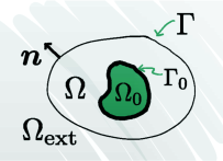
Left: The artificial boundary Γ splits the domain of definition of problem (2.1) into an unbounded region
2.2 Interior and Exterior Problems
To deal with the unboundedness of the domain, later on we will make use of an integral representation that will reduce the computations to a bounded domain. To this avail, we introduce an artificial, smoothly parametrizable interface Γ enclosing
Since we aim to use an integral equation formulation, for the exterior problem we will prefer a second order formulation and will eliminate
where the functions u and
(2.2)
On the other hand, the exterior function
(2.3)
Above, the boundary value
2.3 Boundary Integral Formulation for the Exterior Problem
We will now reformulate (2.3) as a boundary integral equation. To do that, we will make use of some standard results from potential theory; we refer the reader interested in further details to the classic references [13, 18] for a comprehensive account, or to [12] for a more concise treatment.
We start by introducing the single layer and double layer potentials defined respectively for
where
where the jump operator is defined for
In a similar fashion we can define the average operators as
and use them to define the following boundary integral operators:
We are now in a position to recast the exterior problem (2.3) in terms of boundary integral equations. To that avail, we will represent
and extend it by zero for
giving rise to the integral equation
(2.7)
To ensure that
Equation (2.7a) will be used as part of the alternating scheme described in Section 5, where an approximation of λ will be produced by a numerical solution of the interior problem (2.2) and the density g solving (2.7a) will be then used as the Dirichlet datum for (2.2).
Therefore, if Γ has two continuous derivatives and
Moreover, from this estimate and the representation formula (2.6), it follows that there exists
2.4 Variational Formulation for the Interior Problem
In this subsection, we will study the interior Dirichlet boundary value problem obtained from (2.2) by removing (2.2d) altogether and considering that the boundary trace g, appearing in (2.2c), is known. This yields the problem
(2.10)
Above, the source term
To derive the weak formulation of this system, we test (2.10a) with an arbitrary
where
Problem.
Find
(2.11)
where the bilinear forms
The well-posedness of (2.11) follows from standard arguments of Babǔska–Brezzi theory [11, Section 2.4] and the solution satisfies
We will, however, not solve the problem as stated above and instead will consider a slightly different version posed in a subdomain. This approach, known as the transfer path method will be described in detail in Section 3.2, and will require us first to discuss the geometric setting of the discretization, which we will do next.
3 HDG Discretization of the Interior Problem
3.1 Geometric Setting and Notation
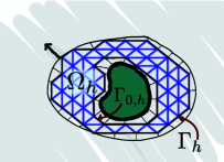
The Computational Domain.
We will consider a family of polygonal subdomains
and those that are either interior or have at most their endpoints in the computational boundary
We will refer to the former as boundary edges and to the latter as interior edges. Note that
Just as the boundary associated to the continuous problem (2.2) has two separate connected components, the boundary of the computational domain can be split as
We will require that the computational domain
Mesh-Dependent Subspaces and Inner Products.
For the discrete formulation we will have introduce the following mesh-dependent inner products:
These inner products induce mesh-dependent norms that will be denoted, respectively, by
The finite-dimensional discontinuous polynomial subspaces that will be used for discretization, for
where
Extension Patches and Extrapolation.
Since the discrete spaces are defined only over the elements of the triangulation we will need to define a way to compute our approximations in the region
Let
Let
Let
We will refer to the open region of
It also follows from this construction that for every
For a given domain
Finally, for every edge
and will define the boundary proximity parameter as
and will assume for this work that the family of admissible domains and triangulations
3.2 Transferal of Boundary Conditions
Having introduced all the necessary geometric concepts we can now return to the interior problem (2.10) which we will now pose in a polygonal computational domain
assigning a point
For any fixed computational domain
(3.2)
where the boundary condition
Note that the required bijectivity of
where the bilinear forms
Beyond the difference in the domain of definition, the system above differs from the original problem (2.11) in the presence of the term
3.3 Discrete Variational Formulation
Having defined all the required notation, we can now state the HDG discretization of (2.10) which, for Dirichlet data
(3.4)
for any test
where E denotes the extrapolation operator.
The numerical flux in the normal direction
where τ stabilization function. Throughout this analysis we will only require
Note that the terms
Replacing now the numerical flux (3.5) in (3.4c) results in
In order to apply known results from functional analysis, we rewrite the numerical trace
Above, we have used the fact that the hybrid variable
in the expression above, we deduce that
We make use of this identity to obtain
and
In this way, replacing the definition of
(3.6)
where the bilinear forms
(3.7)
The unique solvability of the scheme (3.6) will be proved by an energy argument. To that end, for
This norm is equivalent to the standard
This equivalence holds true under certain conditions on the transferring vectors
We also introduce the element-wise constants
where
We now proceed to derive an energy inequality that will lead to the well-posedness of (3.6).
Lemma 1.
Let
Proof.
By taking
First of all, after performing algebraic calculations, we observe that
We will now obtain a lower bound for the non-positive terms of left-hand side of (3.11). In this direction, the operator
where we have used the bound
The same arguments yield to
Therefore, combining the above estimates and (3.11), we deduce that
Finally, the result follows by the discrete trace inequality applied to the boundary terms on the right-hand side, Young’s inequality and the definition of
Corollary 1.
The HDG scheme (3.6) is well-posed for h sufficiently small.
Proof.
Let
Thus, taking
The energy estimate in Lemma 1 provides the stability bound for the vector-valued unknown
where, for convenience of notation of the forthcoming analysis, we have denoted
Having established the well posedness of the discrete formulation, in the following section we will study the behavior of the discretization error.
3.4 A Priori Error Analysis
To establish a priori error bounds for the HDG discretization, we will make use of a tool introduced by Francisco-Javier Sayas, Jay Gopalakrishnan and Bernardo Cockburn in [4]. The idea is to use a projection, known as the HDG projection, to decompose the discretization into a component involving the approximation properties of the discrete spaces
(3.17)
for every element
where
We will now show that the scheme (3.6) is consistent and the discretization error is driven solely by the approximation properties of the discrete spaces, as encoded by
However, since
where in the last equality we have used the fact that
Analogously, from (3.6b) we have
Analyzing the terms above that involve
Putting these arguments together it follows from (3.18) and (3.19) that the scheme is consistent and the following error equations for
(3.20)
Now, by the orthogonality properties of the HDG projection (3.17), we deduce that
and
In this way, we conclude that the projection of the errors
(3.21)
with
and
Theorem 1.
For h sufficiently small, there holds
Moreover, under elliptic regularity it holds
Proof.
By proceeding exactly as in the proof of Lemma 1, but in the context of the equation of the projection of the errors (3.21), for h sufficiently small, we deduce that
where we recall the definition of J in (3.16). In order to bound the terms on the right-hand side, we employ the Cauchy–Schwarz and discrete trace inequalities and obtain that
where we have also used the fact that
Therefore, by combining the above inequalities, we obtain
and (3.22) follows by the fact that
which implies (3.23). ∎
Corollary 2.
If
Moreover, if
Proof.
The first inequality follows from the approximation properties of the HDG projection stated in Section 6. On the other hand,
But, using the approximation estimates (6.1), we have
and (3.25) follows. ∎
4 BEM Discretization of the Exterior Problem
For the discretization of the integral equation (2.7) we will take advantage of the fact that the parametrization of artificial boundary Γ is smooth and does not intersect with the support of the source term. It is a standard result in potential theory that these two conditions imply that the densities λ and g are both
If we let
where the integral kernels are the two-dimensional Green function for the minus Laplacian and its normal derivative, namely
The idea is then to discretize the parameterization of Γ into
For real numbers
where
These functions can be used to build the basis for
If we denote by
where
Therefore, if
Note that the term involving the constant
Hence, we first solve (4.1) for
from which the unique solvability of (4.1) follows. Moreover, for a Galerkin approximation of (4.1) it can be shown [29, Theorem 9.4.1] that the following error estimate holds:
Combining this approximation result with the stability estimate (2.8) and the boundedness of the single layer operator
5 Iterative Coupled Procedure
In Coupling at a distance, the authors proposed an iterative method to find the solution to the original problem (2.1) by alternating between the solutions of the interior and exterior problems using HDG and spectral BEM respectively. The idea can be traced back to [6] and involves using the Dirichlet trace of u over the artificial boundary as the unknown coupling variable and alternating between the solution of an interior and an exterior problem.
We start by observing that, from the discrete version of the transmission condition (2.2d)
the Neumann trace of the exterior problem can be written in terms of its interior counterpart as
where
This algorithm amounts to a Schur complement strategy where the Dirichlet-to-Neumann map (DtN) for the interior problem is approximated via HDG, and the Neumann-to-Dirichlet mapping (NtD) for the exterior problem is approximated via spectral BEM. As we have shown in the previous sections, both of these problems are uniquely and stably solvable, therefore, it remains to show that the iterated composition of these mappings will converge, and that the limits will in fact be the discrete Dirichlet and Neumann traces over Γ of the solution to (2.1).
To explain the procedure at the continuous level we start by fixing
Step 1:
Solve the interior Dirichlet boundary value problem
(5.2)
Step 2:
Solve the boundary integral equation
We can then summarize the algorithm as, staring from an initial boundary datum
What we will show in this section is that, as the distance between Γ and
5.1 Continuous Problem
5.1.1 Fixed Point Operator and Relaxation
We start by introducing the space of admissible Neumann traces for the exterior problem at the continuous level
The Dirichlet to Neumann mapping for the interior problem is then defined as
where
Similarly, we can define the Neumann to Dirichlet map for the exterior problem as
where
The iterative procedure consists on the alternated application of these mappings, and is thus described by the repeated application of the operator
which, by the arguments given above, satisfies the stability estimate
As mentioned earlier, the simple iterative process described in previous section is not convergent in general. However this drawback can be overcome by the introduction of an additional relaxation step and a relaxation parameter
Step 1:
Solve the interior Dirichlet boundary value problem
(5.4)
Step 2:
Solve the boundary integral equation
Step 3:
Update the Dirichlet trace
We will denote the operator mapping a trace g to the update defined by the relaxed process described above by
Lemma 2.
Assume that
Proof.
If g is a fixed point of
5.1.2 Contraction Property of
T
ω
We will now show that the relaxed mapping is indeed a contraction and therefore, by the observation above, the operator T has indeed a fixed point. To do so, we will adapt the ideas applied by Marini and Quarteroni in [17], where they dealt with a primal formulation involving only PDE formulations in the two subdomains.
We are interested in showing that the repeated application of the operator
The problem above is a particular instance of (2.11), which has been shown to be uniquely solvable. Recalling that
This induces a norm over
Moreover, from the definition of
Lemma 3.
The following estimates hold for
Proof.
The first estimate follows readily from the definition of the inner product
For (5.9) we start from (5.7) and make use of the fact that, by construction, Tg satisfies the boundary integral equation (5.2b), leading to
Using now the representation
Combining the last two expressions, we arrive at (5.9). Inequality (5.10) follows readily from (5.8) and (5.9) as follows:
Finally, we will use the fact that
where in the last inequality we have appealed to an argument from [15, 17] pointing to the existence of a positive constant σ such that
and the constant
Using the estimates from the previous lemma, we can now compute
where we have defined
We note that the quantity
This implies that
5.2 Discrete Problem
We will follow the main ideas introduced for the analysis of the continuous counterpart, but we will have to adapt them to account for the additional challenges posed by the discretization and the transfer technique.
5.2.1 Discrete Fixed Point Operator and Relaxation
In this subsection we construct the discrete counterpart of the operators defined in Section 5.1.1. To that end, we let
and define the discrete version of the operator
where
On the other hand, consider a mesh edge
Therefore, the above two estimates imply that there exists
Similarly, the discrete version of the operator
where
We can now define the discrete analogue to the operator T from Section 5.1.1 as
where
5.2.2 Contraction Property of
T
h
,
n
We define the discrete version of (5.6). For
where
Now, expressing the integral over
Therefore, since τ is positive and
and we notice that
We now establish the relationship between the discrete norm
Lemma 4.
Let
Proof.
Let
The following identity and the one in the subsequent corollary establish the connection between the inner product
Lemma 5.
Let
Proof.
Let
Now, since ϕ is a bijective mapping, we write the first term of the right-hand side as follows:
where we have added and subtracted
where we added and subtracted
Gathering all the above identities, we obtain (5). ∎
In the particular case of a circular interface Γ, the integral operators applied to trigonometric polynomials are also trigonometric polynomials. Therefore, we have the following identity.
Corollary 3.
Let us suppose that Γ is a circular interface. For
We recall that the interface Γ has been introduced artificially and its shape can be chosen to facilitate computations. In particular, all the boundary integrals can be explicitly computed in the case of a circular interface. This actually the case of the numerical examples reported in [7]. From now on, for the sake of simplicity of the exposition, we will consider Γ is a circular interface.
The next lemma provides a discrete version of the inequalities presented in Lemma 3.
To that end, let us first notice that the solution u of (2.11) is actually in
Lemma 6.
Let
where
and
with
Moreover,
and
Proof.
To prove (5.23), we start by using the definition of the norm
However, since
which implies (5.24).
Now, let
For the second term on the right-hand side we have that
where in the last inequality we employed (5.20) and the definition of
Now, by setting
and recalling that
On the other hand, (5.25) implies
Then, by (5.24) and Young’s inequality, we obtain
and (5.26) follows.
Finally, taking
which implies (5.27). ∎
Similarly to the case of the operator
We can now use the previous lemmas to prove the main result of this communication, namely the convergence of the iterative procedure.
Theorem 3.
If the mesh parameter h is small enough, it is possible to find values of the relaxation parameter ω in the interval
Proof.
Let
where in the last inequality we made use of (5.24). Then, by (5.27),
where
Analogously to the analysis of the continuous operator, we observe that
with
The extreme value for
Since
We note that for the case of a fitted geometry (i.e. whenever
in coincidence with the continuous case. Above, the presence of the parameter
6 HDG Projection
Given constants
(6.1)
where
Dedicated to the memory of Francisco-Javier Sayas
Funding source: Agencia Nacional de Investigación y Desarrollo
Award Identifier / Grant number: ACE210010 and FB210005
Funding source: National Science Foundation
Award Identifier / Grant number: DMS-2137305
Funding statement: The authors have no relevant financial or non-financial interests to disclose. All authors have contributed equally to the article and the order of authorship has been determined alphabetically. Tonatiuh Sánchez-Vizuet was partially supported by the National Science Foundation through the grant NSF-DMS-2137305 “LEAPS-MPS: Hybridizable discontinuous Galerkin methods for non-linear integro-differential boundary value problems in magnetic plasma confinement”. Manuel Solano was supported by ANID–Chile through Fondecyt 1200569 and by Centro de Modelamiento Matemático (CMM), ACE210010 and FB210005, BASAL funds for center of excellence from ANID-Chile.
References
[1] P. E. Bjørstad and O. B. Widlund, Iterative methods for the solution of elliptic problems on regions partitioned into substructures, SIAM J. Numer. Anal. 23 (1986), no. 6, 1097–1120. 10.1137/0723075Search in Google Scholar
[2] L. Camargo and M. Solano, A high order unfitted HDG method for the Helmholtz equation with first order absorbing boundary condition, preprint 2021-07 (2021), Centro de Investigación en Ingeniería Matemática (CI2MA), Universidad de Concepción, Chile. Search in Google Scholar
[3] C. Canuto and A. Quarteroni, Approximation results for orthogonal polynomials in Sobolev spaces, Math. Comp. 38 (1982), no. 157, 67–86. 10.1090/S0025-5718-1982-0637287-3Search in Google Scholar
[4] B. Cockburn, J. Gopalakrishnan and F.-J. Sayas, A projection-based error analysis of HDG methods, Math. Comp. 79 (2010), no. 271, 1351–1367. 10.1090/S0025-5718-10-02334-3Search in Google Scholar
[5] B. Cockburn, W. Qiu and M. Solano, A priori error analysis for HDG methods using extensions from subdomains to achieve boundary conformity, Math. Comp. 83 (2014), no. 286, 665–699. 10.1090/S0025-5718-2013-02747-0Search in Google Scholar
[6] B. Cockburn and F.-J. Sayas, The devising of symmetric couplings of boundary element and discontinuous Galerkin methods, IMA J. Numer. Anal. 32 (2012), no. 3, 765–794. 10.1093/imanum/drr019Search in Google Scholar
[7] B. Cockburn, F.-J. Sayas and M. Solano, Coupling at a distance HDG and BEM, SIAM J. Sci. Comput. 34 (2012), no. 1, A28–A47. 10.1137/110823237Search in Google Scholar
[8] B. Cockburn and M. Solano, Solving Dirichlet boundary-value problems on curved domains by extensions from subdomains, SIAM J. Sci. Comput. 34 (2012), no. 1, A497–A519. 10.1137/100805200Search in Google Scholar
[9] B. Cockburn and M. Solano, Solving convection-diffusion problems on curved domains by extensions from subdomains, J. Sci. Comput. 59 (2014), no. 2, 512–543. 10.1007/s10915-013-9776-ySearch in Google Scholar
[10] D. Funaro, A. Quarteroni and P. Zanolli, An iterative procedure with interface relaxation for domain decomposition methods, SIAM J. Numer. Anal. 25 (1988), no. 6, 1213–1236. 10.1137/0725069Search in Google Scholar
[11] G. N. Gatica, A Simple Introduction to the Mixed Finite Element Method. Theory and Applications, Springer Briefs Math., Springer, Cham, 2014. 10.1007/978-3-319-03695-3Search in Google Scholar
[12] G. C. Hsiao, O. Steinbach and W. L. Wendland, Boundary Element Methods: Foundation and Error Analysis, John Wiley & Sons, New York, 2017. 10.1002/9781119176817.ecm2007Search in Google Scholar
[13] G. C. Hsiao and W. L. Wendland, Boundary Element Methods: Foundation and Error Analysis. Chapter 12, John Wiley & Sons, New York, 2004. 10.1002/0470091355.ecm007Search in Google Scholar
[14] R. Kress, Linear Integral Equations, 2nd ed., Appl. Math. Sci. 82, Springer, New York, 1999. 10.1007/978-1-4612-0559-3Search in Google Scholar
[15] J.-L. Lions and E. Magenes, Non-Homogeneous Boundary Value Problems and Applications. Vol. I, Grundlehren Math. Wiss. 181, Springer, New York, 1972. 10.1007/978-3-642-65161-8Search in Google Scholar
[16] L. D. Marini and A. Quarteroni, An iterative procedure for domain decomposition methods: a finite element approach, First International Symposium on Domain Decomposition Methods for Partial Differential Equations (Paris 1987), SIAM, Philadelphia (1988), 129–143. Search in Google Scholar
[17] L. D. Marini and A. Quarteroni, A relaxation procedure for domain decomposition methods using finite elements, Numer. Math. 55 (1989), no. 5, 575–598. 10.1007/BF01398917Search in Google Scholar
[18] W. McLean, Strongly Elliptic Systems and Boundary Integral Equations, Cambridge University, Cambridge, 2002. Search in Google Scholar
[19] S. Meddahi and A. Márquez, A combination of spectral and finite elements for an exterior problem in the plane, Appl. Numer. Math. 43 (2002), no. 3, 275–295. 10.1016/S0168-9274(01)00174-XSearch in Google Scholar
[20] R. Oyarzúa, M. Solano and P. Zúñiga, A high order mixed-FEM for diffusion problems on curved domains, J. Sci. Comput. 79 (2019), no. 1, 49–78. 10.1007/s10915-018-0840-5Search in Google Scholar
[21] R. Oyarzúa, M. Solano and P. Zúñiga, A priori and a posteriori error analyses of a high order unfitted mixed-FEM for Stokes flow, Comput. Methods Appl. Mech. Engrg. 360 (2020), Article ID 112780. 10.1016/j.cma.2019.112780Search in Google Scholar
[22] R. Oyarzúa, M. Solano and P. Zúñiga, Analysis of an unfitted mixed finite element method for a class of quasi-Newtonian Stokes flow, Comput. Math. Appl. 114 (2022), 225–243. 10.1016/j.camwa.2022.03.039Search in Google Scholar
[23] W. Qiu, M. Solano and P. Vega, A high order HDG method for curved-interface problems via approximations from straight triangulations, J. Sci. Comput. 69 (2016), no. 3, 1384–1407. 10.1007/s10915-016-0239-0Search in Google Scholar
[24] N. Sánchez, T. Sánchez-Vizuet and M. Solano, Error analysis of an unfitted HDG method for a class of non-linear elliptic problems, J. Sci. Comput. 90 (2022), no. 3, Paper No. 92. 10.1007/s10915-022-01767-1Search in Google Scholar
[25] N. Sánchez, T. Sánchez-Vizuet and M. E. Solano, A priori and a posteriori error analysis of an unfitted HDG method for semi-linear elliptic problems, Numer. Math. 148 (2021), no. 4, 919–958. 10.1007/s00211-021-01221-8Search in Google Scholar
[26] N. Sánchez, T. Sánchez-Vizuet and M. E. Solano, Analysis of a coupled HDG-BEM formulation for non-linear elliptic problems with curved interfaces, in preparation. Search in Google Scholar
[27] T. Sánchez-Vizuet and M. E. Solano, A hybridizable discontinuous Galerkin solver for the Grad–Shafranov equation, Comput. Phys. Commun. 235 (2019), 120–132. 10.1016/j.cpc.2018.09.013Search in Google Scholar
[28] T. Sánchez-Vizuet, M. E. Solano and A. J. Cerfon, Adaptive hybridizable discontinuous Galerkin discretization of the Grad–Shafranov equation by extension from polygonal subdomains, Comput. Phys. Commun. 255 (2020), Article ID 107239. 10.1016/j.cpc.2020.107239Search in Google Scholar
[29] J. Saranen and G. Vainikko, Periodic Integral and Pseudodifferential Equations with Numerical Approximation, Springer Monogr. Math., Springer, Berlin, 2002. 10.1007/978-3-662-04796-5Search in Google Scholar
[30] S. A. Sauter and C. Schwab, Boundary Element Methods, Springer Ser. Comput. Math. 39, Springer, Berlin, 2011. 10.1007/978-3-540-68093-2Search in Google Scholar
[31] M. Solano, S. Terrana, N.-C. Nguyen and J. Peraire, An HDG method for dissimilar meshes, IMA J. Numer. Anal. 42 (2022), no. 2, 1665–1699. 10.1093/imanum/drab059Search in Google Scholar
[32] M. Solano and F. Vargas, A high order HDG method for Stokes flow in curved domains, J. Sci. Comput. 79 (2019), no. 3, 1505–1533. 10.1007/s10915-018-00901-2Search in Google Scholar
[33] M. Solano and F. Vargas, An unfitted HDG method for Oseen equations, J. Comput. Appl. Math. 399 (2022), Paper No. 113721. 10.1016/j.cam.2021.113721Search in Google Scholar
© 2022 Walter de Gruyter GmbH, Berlin/Boston
Articles in the same Issue
- Frontmatter
- Numerical Analysis & No Regrets. Special Issue Dedicated to the Memory of Francisco Javier Sayas (1968–2019)
- Implicit/Explicit, BEM/FEM Coupled Scheme for Acoustic Waves with the Wave Equation in the Second Order Formulation
- Discontinuous Galerkin Methods with Time-Operators in Their Numerical Traces for Time-Dependent Electromagnetics
- A Discontinuous Galerkin Method for the Stationary Boussinesq System
- Korn’s Inequality and Eigenproblems for the Lamé Operator
- Error Estimates for FE-BE Coupling of Scattering of Waves in the Time Domain
- An Efficient Numerical Method for Time Domain Electromagnetic Wave Propagation in Co-axial Cables
- The Time Domain Linear Sampling Method for Determining the Shape of Multiple Scatterers Using Electromagnetic Waves
- A Boundary Integral Formulation and a Topological Energy-Based Method for an Inverse 3D Multiple Scattering Problem with Sound-Soft, Sound-Hard, Penetrable, and Absorbing Objects
- Afternote to “Coupling at a Distance”: Convergence Analysis and A Priori Error Estimates
- Spurious Resonances in Coupled Domain-Boundary Variational Formulations of Transmission Problems in Electromagnetism and Acoustics
- Spectral, Tensor and Domain Decomposition Methods for Fractional PDEs