Superconvergent DPG Methods for Second-Order Elliptic Problems
-
Thomas Führer


Abstract
We consider DPG methods with optimal test functions and broken test spaces based on ultra-weak formulations of general
second-order elliptic problems.
Under some assumptions on the regularity of solutions of the model problem and its adjoint, superconvergence for the
scalar field variable is achieved by either increasing the polynomial degree in the corresponding approximation space by
one or by a local postprocessing.
We provide a uniform analysis that allows the treatment of different test norms.
Particularly, we show that in the presence of convection only the quasi-optimal test norm leads to higher convergence
rates, whereas other norms considered do not.
Moreover, we also prove that our DPG method delivers the best
1 Introduction
In this work we investigate convergence rates of DPG methods based on an ultra-weak formulation of second-order elliptic problems stated in the form of the general first-order system
(1.1)
where
which implies that for
In this work we consider DPG methods with optimal test functions and broken test spaces,
which have been introduced by Demkowicz and Gopalakrishnan, see [5, 6] and also [8, 22].
For a unified stability analysis which also covers our model problem we refer to [3].
We analyze ultra-weak formulations of (1.1), which
are obtained by multiplying with locally supported functions and integration
by parts, see, e.g., [7] for a Poisson model problem.
On the one hand, this has the advantage that the field variables can be sought in
The motivation of this work is to analyze superconvergence properties for approximations of the scalar field variable
u that have been observed in our recent work [10] for a simple reaction-diffusion problem, where
Let us also mention the recent works [14, 15] that deal with dual
problems in the context of DPG methods (the DPG
1.1 Summary of Results
We seek approximations
where
Augmenting the trial space: Instead of seeking approximations
Based on similar techniques we also provide a proof of the following:
DPG for ultra-weak formulations delivers the
where
The latter observation is quite interesting, because it shows that even though we do not aim for higher convergence rates (by increasing the polynomial degree in the trial space or by postprocessing) we get highly accurate approximations. We stress that this result has been observed in various numerical experiments, particularly also for more complex model problems like Stokes [17], but up to now a rigorous proof has not been given.
If
1.2 Basic Ideas
For the proofs of the main results, we develop duality arguments and show approximation results
(Lemma 8 and Lemma 10).
To get the essential idea, consider the abstract formulation: Find
where U denotes the trial space and V the test space. With the trial-to-test operator
the ideal DPG method reads: Find
Then we solve a dual problem:
For some given
for arbitrary
For the case where we want to show that the approximation
The latter estimate is what we have to show. Suppose that it holds. With the estimate for
Let us come back to the essential estimate
It holds if we would know that
the higher derivatives of
by some standard arguments. In our case we have that
where components of
Let us note that Θ is defined through the inner product in the test space. Thus,
the representation of
Moreover, the ideas so far dealt with the ideal DPG method. In this paper we work out all results for the practical DPG method under standard assumptions, i.e., the existence of Fortin operators. This implies that we have to deal with additional discretization errors.
Finally, we note that higher convergence rates for the dual variable
are less regular than in the case described above.
1.3 Outline
The remainder of the paper is organized as follows: Section 2 introduces basic notations, states the assumptions, and presents the main results (Theorem 3–5). The proofs of these theorems are postponed to Section 3, which also includes an a priori convergence estimate (Theorem 6) and the important auxiliary results Lemma 8, 10. In Section 4 we present two numerical experiments. The final Section 5 concludes this work with some remarks.
2 Main Results
2.1 Notation
We make use of the notation
2.2 Mesh
Let
where
2.3 Ultra-Weak Formulation
Before we derive the ultra-weak formulation of (1.1) in this subsection, we introduce some notation.
Let
where
These Hilbert spaces are equipped with minimum energy extension norms
We use the broken test spaces
and define the piecewise differential operators
Moreover, we define the following dualities for all
These dualities measure the jumps of
(2.1)
see, e.g., [3, Theorem 2.3].
The ultra-weak formulation is then derived from (1.1) by testing (1.1a) with
Here,
and define
for all
2.4 DPG Method and Approximation
In U we use the canonical norm,
For the test space V we define the three different norms
(2.3)
for
We stress that
The DPG method seeks an approximation
Then
An essential feature of DPG is that
Then the practical DPG method reads: Find
In this work we deal with the piecewise polynomial trial spaces
and the piecewise polynomial test spaces
Here, we set
where
is the space of Raviart–Thomas functions (here
We also use the space
2.5 Fortin Operators
It is well known, see, e.g., [12], that (2.5) satisfies
Throughout, we suppose that a Fortin operator exists for the discrete polynomial trial and test spaces under
consideration and that
Supposing the existence of an Fortin operator, i.e., (2.6), we have:
2.6 Adjoint Problem and Regularity Assumptions
We define the adjoint problem (in the sense of
(2.7)
Supposing (1.2) this problem admits a unique solution
For our results we make use of the following assumptions:
Assumption.
We suppose that the coefficients
(2.8)
Here,
Remark 2.
The regularity estimates (2.8) are satisfied if
Then
Similarly, one shows (2.8b) (even a less regular coefficient
2.7 Assumptions on Coefficients and Test Norms
Besides the assumptions on the coefficients and the domain to ensure unique solvability of
problems (1.1) and (2.7) and estimates (2.8), we also need some
additional assumptions on the coefficients that are listed in Table 1.
We emphasize that
2.8 L 2 ( Ω )
Our first main result shows that the DPG method with ultra-weak formulation delivers up to a higher-order term the
Theorem 3.
Consider one of Cases (a), (b), or (c).
Let
The constant
2.9 Higher Convergence Rate by Increasing Polynomial Degree
Our second main result shows that higher convergence rates for the scalar field variable are obtained by increasing the polynomial degree in the approximation space.
Theorem 4.
Consider one of Cases (a), (b), or (c).
Let
The constant
2.10 Higher Convergence Rate by Postprocessing
Our third and final main result shows that higher convergence rates for the scalar field variable are obtained by
postprocessing the solution:
Let
(2.9)
Let us note that this type of postprocessing is common in literature and can already be found in the early works [11, 20].
Theorem 5.
Consider one of Cases (a), (b), or (c).
Let
The constant
3 Proofs
In this section we prove the results stated in Theorems 3, 4, and 5.
First, in Section 3.1 we collect some standard results on projection operators and consider approximation
results with respect to
3.1 Projection Operators and Approximation Results
Throughout let
(3.1)
where
denote the Scott–Zhang projection operator [19] or any other operator with the property
Moreover, let
and the commutativity property
Note that
The following result is an adaptation of [10, Theorem 5 and Corollary 6].
Theorem 6.
Let
The constant
Proof.
Define
We estimate the terms in
First, we follow [10, Proof of Theorem 5] to estimate
Then elementwise integration by parts and the commutativity property yield
Using the
Putting the last estimates together this shows that
Next, observe that
Remark 7.
As pointed out in [10] the estimate
Using the commutativity property and the approximation properties (3.1a), (3.1c) we get
Thus, in order to get the same convergence rate as in Theorem 6 we have to assume the higher regularity
3.2 Mixed Formulation of the Practical DPG Method
The practical DPG method (2.5) can be reformulated as a mixed problem, see,
e.g., [1]. Recall that we made the assumption of the existence of a Fortin
operator (2.6).
The mixed DPG formulation then reads:
Find
(3.2)
The Riesz representation
under assumption (2.6), see [2, Theorem 2.1].
Note that the solution
where
3.3 Auxiliary Results
Recall the adjoint problem (2.7) with
Note that
Lemma 8.
Let
Case (a) (
where
Case (b) (
where
Case (c) (
where
Moreover,
For Case (c) it also holds that
Proof.
We consider the three cases. Case (a). Recall that
With the inner product in V and
Let
Defining
Thus,
Case (b). The scalar product in this case is given by
Recall that
With
Thus,
Defining
where
Case (c).
The proof is similar as for Case (b). Thus, we only give details on the important differences.
We have to take care of the terms involving the matrix
and using
Defining
where
Finally, note that for all three cases it is straightforward to prove
Then (2.8) shows estimate (3.4). Moreover, in Case (c) we have
Remark 9.
As already mentioned in the introduction, in the recent work [15] the optimal test norm
is considered and the problem of finding
Lemma 10.
Consider one of Cases (a)–(c).
Let
It holds that
The constant
Proof.
Let
With the bilinear form
we infer
Here,
It remains to prove
We start with the estimation of
Then, using the approximation properties (3.1) together with (3.4), we get
Then, for the remaining term the commutativity property of the Raviart–Thomas projection, the adjoint
problem (3.3) and
Using the approximation properties of
Therefore, we obtain
It only remains to estimate
Case (a).
By Lemma 8 we have
where
Case (b).
By Lemma 8 we have
where
where we used (3.1) and the approximation property of
Case (c). The proof follows as for Case (b). Therefore, we omit the details. ∎
3.4 Proof of Theorem 3
The best approximation property of
With
We apply Lemma 10, and the approximation result from Theorem 6 to see
Dividing by
which finishes the proof.
3.5 Proof of Theorem 4
The proof is similar to the one for Theorem 3. We consider
Define
This finishes the proof.
3.6 Proof of Theorem 5
Note that (2.9b) is equivalent to
where we have used the local approximation property of
It remains to estimate
for all
To estimate
Hence, standard approximation results show
Putting altogether gives
which finishes the proof.
4 Numerical Studies
In this section we present results of two numerical examples.
Let
which is smooth and satisfies
Let
To verify our main results (Theorem 3, Theorem 4, and Theorem 5), we check
the convergence rates of the
All computations start with the initial triangulation
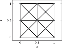
Initial triangulation
4.1 Example 1
Define
Moreover, we choose
Note that
4.2 Example 2
For this example we choose
Note that
Errors and rates for the problem from Section 4.1 with test norm
| p | rate | rate | rate | rate | |||||
| 0 | 16 | 1.94e | – | 7.41e | – | 8.37e | – | 1.23e | – |
| 64 | 9.37e | 1.05 | 1.85e | 2.00 | 2.09e | 2.01 | 3.21e | 1.94 | |
| 256 | 4.64e | 1.01 | 4.63e | 2.00 | 5.20e | 2.00 | 8.12e | 1.98 | |
| 1024 | 2.32e | 1.00 | 1.16e | 2.00 | 1.30e | 2.00 | 2.04e | 2.00 | |
| 4096 | 1.16e | 1.00 | 2.90e | 2.00 | 3.25e | 2.00 | 5.09e | 2.00 | |
| 16384 | 5.79e | 1.00 | 7.24e | 2.00 | 8.13e | 2.00 | 1.27e | 2.00 | |
| 65536 | 2.89e | 1.00 | 1.81e | 2.00 | 2.03e | 2.00 | 3.18e | 2.00 | |
| 1 | 16 | 3.47e | – | 3.02e | – | 5.96e | – | 7.89e | – |
| 64 | 8.86e | 1.97 | 5.58e | 2.44 | 8.72e | 2.77 | 9.53e | 3.05 | |
| 256 | 2.22e | 1.99 | 7.92e | 2.82 | 1.16e | 2.92 | 1.18e | 3.01 | |
| 1024 | 5.56e | 2.00 | 1.02e | 2.95 | 1.47e | 2.98 | 1.48e | 3.00 | |
| 4096 | 1.39e | 2.00 | 1.29e | 2.99 | 1.84e | 2.99 | 1.84e | 3.00 | |
| 16384 | 3.48e | 2.00 | 1.62e | 3.00 | 2.31e | 3.00 | 2.30e | 3.00 | |
| 2 | 16 | 4.51e | – | 2.55e | – | 3.51e | – | 6.14e | – |
| 64 | 5.74e | 2.98 | 1.30e | 4.29 | 1.98e | 4.14 | 4.18e | 3.88 | |
| 256 | 7.20e | 2.99 | 7.67e | 4.09 | 1.21e | 4.04 | 2.68e | 3.96 | |
| 1024 | 9.01e | 3.00 | 4.72e | 4.02 | 7.50e | 4.01 | 1.68e | 3.99 | |
| 4096 | 1.13e | 3.00 | 2.97e | 3.99 | 4.69e | 4.00 | 1.05e | 4.00 | |
| 3 | 16 | 2.20e | – | 2.08e | – | 2.01e | – | 5.48e | – |
| 64 | 1.39e | 3.98 | 8.34e | 4.64 | 8.38e | 4.58 | 1.67e | 5.03 | |
| 256 | 8.70e | 4.00 | 2.82e | 4.89 | 2.86e | 4.87 | 5.18e | 5.01 | |
| 1024 | 5.44e | 4.00 | 9.08e | 4.96 | 9.24e | 4.95 | 1.62e | 5.00 |
Errors and rates for the problem from Section 4.1 with test norm
| p | rate | rate | rate | rate | |||||
| 0 | 16 | 1.92e | – | 6.88e | – | 7.86e | – | 8.48e | – |
| 64 | 9.35e | 1.04 | 1.73e | 1.99 | 1.97e | 1.99 | 2.17e | 1.97 | |
| 256 | 4.64e | 1.01 | 4.33e | 2.00 | 4.94e | 2.00 | 5.44e | 1.99 | |
| 1024 | 2.32e | 1.00 | 1.08e | 2.00 | 1.23e | 2.00 | 1.36e | 2.00 | |
| 4096 | 1.16e | 1.00 | 2.71e | 2.00 | 3.09e | 2.00 | 3.41e | 2.00 | |
| 16384 | 5.79e | 1.00 | 6.77e | 2.00 | 7.71e | 2.00 | 8.51e | 2.00 | |
| 65536 | 2.89e | 1.00 | 1.69e | 2.00 | 1.93e | 2.00 | 2.13e | 2.00 | |
| 1 | 16 | 3.49e | – | 4.81e | – | 6.96e | – | 6.79e | – |
| 64 | 8.87e | 1.98 | 7.36e | 2.71 | 9.71e | 2.84 | 8.82e | 2.95 | |
| 256 | 2.22e | 2.00 | 9.82e | 2.91 | 1.26e | 2.95 | 1.12e | 2.98 | |
| 1024 | 5.56e | 2.00 | 1.25e | 2.97 | 1.59e | 2.99 | 1.41e | 2.99 | |
| 4096 | 1.39e | 2.00 | 1.57e | 2.99 | 1.99e | 3.00 | 1.76e | 3.00 | |
| 16384 | 3.48e | 2.00 | 1.96e | 3.00 | 2.49e | 3.00 | 2.20e | 3.00 | |
| 2 | 16 | 4.53e | – | 4.38e | – | 5.07e | – | 5.22e | – |
| 64 | 5.74e | 2.98 | 2.53e | 4.11 | 3.00e | 4.08 | 3.25e | 4.01 | |
| 256 | 7.20e | 2.99 | 1.54e | 4.04 | 1.85e | 4.02 | 2.03e | 4.00 | |
| 1024 | 9.01e | 3.00 | 9.58e | 4.01 | 1.15e | 4.01 | 1.27e | 4.00 | |
| 4096 | 1.13e | 3.00 | 6.03e | 3.99 | 7.22e | 3.99 | 7.94e | 4.00 | |
| 3 | 16 | 2.25e | – | 5.14e | – | 5.06e | – | 6.01e | – |
| 64 | 1.40e | 4.01 | 1.75e | 4.88 | 1.73e | 4.87 | 1.96e | 4.94 | |
| 256 | 8.71e | 4.00 | 5.62e | 4.96 | 5.55e | 4.96 | 6.20e | 4.98 | |
| 1024 | 5.44e | 4.00 | 1.80e | 4.96 | 1.78e | 4.96 | 1.96e | 4.98 |
Errors and rates for the problem from Section 4.2 with test norm
| p | rate | rate | rate | rate | |||||
| 0 | 16 | 1.96e | – | 7.95e | – | 8.85e | – | 1.27e | – |
| 64 | 9.41e | 1.06 | 2.04e | 1.96 | 2.25e | 1.98 | 3.36e | 1.92 | |
| 256 | 4.65e | 1.02 | 5.14e | 1.99 | 5.64e | 1.99 | 8.51e | 1.98 | |
| 1024 | 2.32e | 1.00 | 1.29e | 2.00 | 1.41e | 2.00 | 2.13e | 1.99 | |
| 4096 | 1.16e | 1.00 | 3.22e | 2.00 | 3.53e | 2.00 | 5.34e | 2.00 | |
| 16384 | 5.79e | 1.00 | 8.05e | 2.00 | 8.82e | 2.00 | 1.34e | 2.00 | |
| 65536 | 2.89e | 1.00 | 2.01e | 2.00 | 2.21e | 2.00 | 3.34e | 2.00 | |
| 1 | 16 | 3.47e | – | 2.77e | – | 5.91e | – | 8.02e | – |
| 64 | 8.85e | 1.97 | 5.22e | 2.40 | 8.59e | 2.78 | 9.73e | 3.04 | |
| 256 | 2.22e | 1.99 | 7.47e | 2.80 | 1.14e | 2.92 | 1.21e | 3.01 | |
| 1024 | 5.56e | 2.00 | 9.69e | 2.95 | 1.44e | 2.98 | 1.51e | 3.00 | |
| 4096 | 1.39e | 2.00 | 1.22e | 2.99 | 1.81e | 2.99 | 1.89e | 3.00 | |
| 16384 | 3.48e | 2.00 | 1.53e | 3.00 | 2.27e | 3.00 | 2.36e | 3.00 | |
| 2 | 16 | 4.51e | – | 2.37e | – | 3.44e | – | 6.25e | – |
| 64 | 5.73e | 2.98 | 1.19e | 4.32 | 1.95e | 4.14 | 4.24e | 3.88 | |
| 256 | 7.20e | 2.99 | 6.97e | 4.09 | 1.19e | 4.04 | 2.72e | 3.97 | |
| 1024 | 9.01e | 3.00 | 4.28e | 4.02 | 7.37e | 4.01 | 1.71e | 3.99 | |
| 4096 | 1.13e | 3.00 | 2.68e | 4.00 | 4.60e | 4.00 | 1.07e | 4.00 | |
| 3 | 16 | 2.20e | – | 1.95e | – | 1.98e | – | 5.51e | – |
| 64 | 1.39e | 3.98 | 7.80e | 4.64 | 8.14e | 4.61 | 1.68e | 5.04 | |
| 256 | 8.70e | 4.00 | 2.65e | 4.88 | 2.78e | 4.87 | 5.21e | 5.01 | |
| 1024 | 5.44e | 4.00 | 8.73e | 4.92 | 9.16e | 4.92 | 1.63e | 5.00 |
Errors and rates for the problem from Section 4.2 with test norm
| p | rate | rate | rate | rate | |||||
| 0 | 16 | 4.37e | – | 3.98e | – | 4.15e | – | 4.00e | – |
| 64 | 2.25e | 0.96 | 2.06e | 0.95 | 2.14e | 0.96 | 2.06e | 0.96 | |
| 256 | 1.14e | 0.99 | 1.04e | 0.98 | 1.08e | 0.99 | 1.04e | 0.99 | |
| 1024 | 5.70e | 1.00 | 5.21e | 1.00 | 5.41e | 1.00 | 5.21e | 1.00 | |
| 4096 | 2.85e | 1.00 | 2.61e | 1.00 | 2.71e | 1.00 | 2.61e | 1.00 | |
| 16384 | 1.43e | 1.00 | 1.30e | 1.00 | 1.35e | 1.00 | 1.30e | 1.00 | |
| 65536 | 7.13e | 1.00 | 6.52e | 1.00 | 6.77e | 1.00 | 6.52e | 1.00 | |
| 1 | 16 | 6.23e | – | 5.18e | – | 5.69e | – | 1.64e | – |
| 64 | 1.63e | 1.93 | 1.37e | 1.92 | 1.49e | 1.93 | 5.70e | 1.52 | |
| 256 | 4.12e | 1.98 | 3.47e | 1.98 | 3.77e | 1.98 | 1.61e | 1.83 | |
| 1024 | 1.03e | 2.00 | 8.67e | 2.00 | 9.42e | 2.00 | 4.19e | 1.94 | |
| 4096 | 2.57e | 2.00 | 2.17e | 2.00 | 2.35e | 2.00 | 1.06e | 1.98 | |
| 16384 | 6.43e | 2.00 | 5.41e | 2.00 | 5.88e | 2.00 | 2.68e | 1.99 | |
| 2 | 16 | 7.46e | – | 5.95e | – | 6.56e | – | 9.34e | – |
| 64 | 9.32e | 3.00 | 7.35e | 3.02 | 8.17e | 3.00 | 6.23e | 3.91 | |
| 256 | 1.17e | 3.00 | 9.17e | 3.00 | 1.02e | 3.00 | 4.01e | 3.96 | |
| 1024 | 1.46e | 3.00 | 1.15e | 3.00 | 1.28e | 3.00 | 2.57e | 3.96 | |
| 4096 | 1.82e | 3.00 | 1.43e | 3.00 | 1.59e | 3.00 | 1.66e | 3.95 | |
| 3 | 16 | 6.03e | – | 5.62e | – | 5.59e | – | 7.46e | – |
| 64 | 3.88e | 3.96 | 3.63e | 3.95 | 3.64e | 3.94 | 3.93e | 4.25 | |
| 256 | 2.44e | 3.99 | 2.28e | 3.99 | 2.29e | 3.99 | 2.41e | 4.03 | |
| 1024 | 1.52e | 4.00 | 1.42e | 4.00 | 1.43e | 4.00 | 1.52e | 3.99 |
5 Concluding Remarks
We conclude this work with some remarks.
The results and their proofs are presented in a systematic way that allow
to extend and transfer them to other types of meshes and different model problems.
In principle, the crucial results Lemma 8 and Lemma 10 have to be verified.
Consider for instance that
which is an optimal a priori error bound for sufficient regular functions (see Lemma 10 for details on the definition of
the functions
Future research will include other model problems, e.g., linear elasticity.
Another possible application of the developed ideas could be to the Stokes problem. Consider its
velocity-gradient-pressure formulation: Find
DPG methods based on ultra-weak formulations are known and thoroughly analyzed [17].
Since regularity theory is also known, our main results (Theorem 3–5) should carry over (for the
velocity variable
Another point we like to mention is that the principal ideas of the proofs and, thus, our main results carry
over to the low regularity case, i.e., when we do not have the “full” regularity
Finally, let us remark the importance of the choice of norms in the test space.
Although all test norms under consideration are equivalent and, thus, the
corresponding DPG methods have the same stability properties (i.e., the
Funding source: Fondo Nacional de Desarrollo Científico y Tecnológico
Award Identifier / Grant number: 11170050
Funding statement: This work was supported by FONDECYT project 11170050.
References
[1] T. Bouma, J. Gopalakrishnan and A. Harb, Convergence rates of the DPG method with reduced test space degree, Comput. Math. Appl. 68 (2014), no. 11, 1550–1561. 10.1016/j.camwa.2014.08.004Search in Google Scholar
[2] C. Carstensen, L. Demkowicz and J. Gopalakrishnan, A posteriori error control for DPG methods, SIAM J. Numer. Anal. 52 (2014), no. 3, 1335–1353. 10.1137/130924913Search in Google Scholar
[3] C. Carstensen, L. Demkowicz and J. Gopalakrishnan, Breaking spaces and forms for the DPG method and applications including Maxwell equations, Comput. Math. Appl. 72 (2016), no. 3, 494–522. 10.1016/j.camwa.2016.05.004Search in Google Scholar
[4] B. Cockburn, B. Dong and J. Guzmán, A superconvergent LDG-hybridizable Galerkin method for second-order elliptic problems, Math. Comp. 77 (2008), no. 264, 1887–1916. 10.1090/S0025-5718-08-02123-6Search in Google Scholar
[5] L. Demkowicz and J. Gopalakrishnan, A class of discontinuous Petrov–Galerkin methods. Part I: The transport equation, Comput. Methods Appl. Mech. Engrg. 199 (2010), no. 23–24, 1558–1572. 10.1016/j.cma.2010.01.003Search in Google Scholar
[6] L. Demkowicz and J. Gopalakrishnan, A class of discontinuous Petrov–Galerkin methods. II. Optimal test functions, Numer. Methods Partial Differential Equations 27 (2011), no. 1, 70–105. 10.1002/num.20640Search in Google Scholar
[7] L. Demkowicz and J. Gopalakrishnan, Analysis of the DPG method for the Poisson equation, SIAM J. Numer. Anal. 49 (2011), no. 5, 1788–1809. 10.1137/100809799Search in Google Scholar
[8] L. Demkowicz, J. Gopalakrishnan and A. H. Niemi, A class of discontinuous Petrov–Galerkin methods. Part III: Adaptivity, Appl. Numer. Math. 62 (2012), no. 4, 396–427. 10.1016/j.apnum.2011.09.002Search in Google Scholar
[9] A. Demlow, Suboptimal and optimal convergence in mixed finite element methods, SIAM J. Numer. Anal. 39 (2002), no. 6, 1938–1953. 10.1137/S0036142900376900Search in Google Scholar
[10] T. Führer, Superconvergence in a DPG method for an ultra-weak formulation, Comput. Math. Appl. 75 (2018), no. 5, 1705–1718. 10.1016/j.camwa.2017.11.029Search in Google Scholar
[11] L. Gastaldi and R. H. Nochetto, Sharp maximum norm error estimates for general mixed finite element approximations to second order elliptic equations, RAIRO Modél. Math. Anal. Numér. 23 (1989), no. 1, 103–128. 10.1051/m2an/1989230101031Search in Google Scholar
[12] J. Gopalakrishnan and W. Qiu, An analysis of the practical DPG method, Math. Comp. 83 (2014), no. 286, 537–552. 10.1090/S0025-5718-2013-02721-4Search in Google Scholar
[13] P. Grisvard, Elliptic Problems in Nonsmooth Domains, Monogr. Stud. Math. 24, Pitman, Boston, 1985. Search in Google Scholar
[14]
B. Keith, L. Demkowicz and J. Gopalakrishnan,
[15] B. Keith, A. Vaziri Astaneh and L. Demkowicz, Goal-oriented adaptive mesh refinement for non-symmetric functional settings, preprint (2017), https://arxiv.org/abs/1711.01996. Search in Google Scholar
[16] S. Nagaraj, S. Petrides and L. F. Demkowicz, Construction of DPG Fortin operators for second order problems, Comput. Math. Appl. 74 (2017), no. 8, 1964–1980. 10.1016/j.camwa.2017.05.030Search in Google Scholar
[17] N. V. Roberts, T. Bui-Thanh and L. Demkowicz, The DPG method for the Stokes problem, Comput. Math. Appl. 67 (2014), no. 4, 966–995. 10.1016/j.camwa.2013.12.015Search in Google Scholar
[18] N. V. Roberts, L. Demkowicz and R. Moser, A discontinuous Petrov–Galerkin methodology for adaptive solutions to the incompressible Navier–Stokes equations, J. Comput. Phys. 301 (2015), 456–483. 10.1016/j.jcp.2015.07.014Search in Google Scholar
[19] L. R. Scott and S. Zhang, Finite element interpolation of nonsmooth functions satisfying boundary conditions, Math. Comp. 54 (1990), no. 190, 483–493. 10.1090/S0025-5718-1990-1011446-7Search in Google Scholar
[20] R. Stenberg, Postprocessing schemes for some mixed finite elements, RAIRO Modél. Math. Anal. Numér. 25 (1991), no. 1, 151–167. 10.1051/m2an/1991250101511Search in Google Scholar
[21] A. Vaziri Astaneh, F. Fuentes, J. Mora and L. Demkowicz, High-order polygonal discontinuous Petrov–Galerkin (PolyDPG) methods using ultraweak formulations, Comput. Methods Appl. Mech. Engrg. 332 (2018), 686–711. 10.1016/j.cma.2017.12.011Search in Google Scholar
[22] J. Zitelli, I. Muga, L. Demkowicz, J. Gopalakrishnan, D. Pardo and V. M. Calo, A class of discontinuous Petrov–Galerkin methods. Part IV: the optimal test norm and time-harmonic wave propagation in 1D, J. Comput. Phys. 230 (2011), no. 7, 2406–2432. 10.1016/j.jcp.2010.12.001Search in Google Scholar
© 2019 Walter de Gruyter GmbH, Berlin/Boston
Articles in the same Issue
- Frontmatter
- Special Issue Articles on Minimum Residual and Least-Squares Finite Element Methods
- Recent Advances in Least-Squares and Discontinuous Petrov–Galerkin Finite Element Methods
- A Non-conforming Saddle Point Least Squares Approach for an Elliptic Interface Problem
- Least-Squares Methods for Elasticity and Stokes Equations with Weakly Imposed Symmetry
- Adaptive Strategies for Transport Equations
- Space-Time Discontinuous Petrov–Galerkin Methods for Linear Wave Equations in Heterogeneous Media
- Superconvergent DPG Methods for Second-Order Elliptic Problems
- The Convection-Diffusion-Reaction Equation in Non-Hilbert Sobolev Spaces: A Direct Proof of the Inf-Sup Condition and Stability of Galerkin’s Method
- Fast Integration of DPG Matrices Based on Sum Factorization for all the Energy Spaces
- The Discrete-Dual Minimal-Residual Method (DDMRes) for Weak Advection-Reaction Problems in Banach Spaces
- Camellia: A Rapid Development Framework for Finite Element Solvers
- Alternative Enriched Test Spaces in the DPG Method for Singular Perturbation Problems
- A Newton Div-Curl Least-Squares Finite Element Method for the Elliptic Monge–Ampère Equation
- The Discrete Steklov–Poincaré Operator Using Algebraic Dual Polynomials
- Regular Research Articles
- A Posteriori Error Estimation for Planar Linear Elasticity by Stress Reconstruction
- A Second-Order Time-Stepping Scheme for Simulating Ensembles of Parameterized Flow Problems