The “Stagflation” Risk and Policy Control: Causes, Governance and Inspirations
-
Zhenxia Wang

Abstract
The blend of economic stagnation and inflation is a challenge to the contemporary macroeconomic study. The causes, influence and policy implications of “stagflation” have been academically controversial. This paper starts with the connections between energy crises and stagflation to research the causes of “stagflation” in the 1970s and analyze the realistic impact of energy crises. It then comparatively studies the current economic landscape and the landscape in the 1970s for similarities and differences, digs into the origin of the current macroeconomic situation, and on such basis proposes policy suggestions.
1 Causes of “Stagflation” in History
In the 1960s, British Chancellor of the Exchequer Iain Macleod pointed out in a parliament lecture two adverse situations with the economic development, high inflation and sluggish economic growth, which were in a blend and led to “stagflation”. In the 1970s, major countries in the world were all caught in the “stagflation” with parallel high unemployment, high inflation and low growth, posing profound influence. Since the 1970s, countries have all experienced “stagflation” or “quasi-stagflation” in different periods, but causes of “stagflation” remain controversial in the academic community. Today, the complex international economic and political situations, the lingering impact of COVID-19 and the coinciding Russia-Ukraine war make the prospect of world economic recovery bleak. The world economy currently seems to be in a position similar to the 1970s, possibly expecting the risk of “stagflation” again. In this sense, to comprehensively analyze the causes of “stagflation” in history in depth and draw experience and lessons from the countermeasures is highly inspirational.
1.1 The Energy Crisis and the “Stagflation” in the 1970s
If economic crises have signs, an unmistakable sign is false prosperity prior tocrisis outbreak. Before the world financial crisis in 2008, major countries worldwide saw their real estate and stock market upsurging and consumption rapidly growing and kept loosening economic control and monetary policy, brewing the bubbles and the crisis. Before the “stagflation” in the 1970s, however, the world economy was truly growing. After the end of the Second World War, major countries in the world faced the universal problems of financial strain for development, broken economic and trade systems and highly unstable political order. In response, the countries worked together and put into place the post-war world trade system and financial system, and encouraged production, life and social order to recover, greatly releasing the investment and consumer demand after years of austerity. With the support of all accommodative policies, the world economy grew at an unprecedented rate. According to statistics, from 1950 to 1973, global per capita income growth was 2.92% annually on average, at which rate per capita living standards would double in 25 years (Maddison, 2003). The countries generally had high expectations for future economic growth and social welfare efforts also improved people’s well-being. It’s this reason that makes the root causes of “stagflation” at the time controversial today.
In 1973, the oil crisis broke out and international oil price soon surged. Economy, after decades of rapid growth, soon declined, and developed countries were generally reduced to lasting and persistent economic recession along with continuing high inflation and high unemployment. According to statistics,[1] US per capita GDP growth was averaged at 2.64% from 1962 to 1973, but dropped to 0.55% from 1973 to 1982; in the same period, the growth fell from 7.31% to 2.64% in Japan, from 4.11% to 1.94% in France, and from 2.43% to 0.68% in UK. In the same period, general price level rose from average 3.18% to 8.13% in the US, from 5.13% to 6.34% in Japan, from 3.93% to 11.09% in France, and from 4.72% to 14.93% in UK. Unemployment rate climbed from 4.9% to 6.99% in the US, from 1.13% to 1.94% in Japan, from 1.51% to 4.5% in France and from 1.98% to 5.61% in UK.
A look at the timeline tended to attribute occurrence of the “stagflation” to the supply shock as a result of the surging crude oil price; in another word, because of the fast-rising oil price, manufacturing faced higher cost and the risk of production interruption. Research found out of the eight economic recessions in the US after the Second World War, seven were connected with oil price shock, and the connections were not coincidence in time, but actually existed (Hamilton, 1983). In an economic environment where industrial manufacturing accounted for a high proportion, higher energy price would stifle economic growth by increasing production cost, triggering inflation (expected) and even slowing down technical progress (Burbidge and Harrison, 1984; Gisser and Goodwin, 1986; Mork, 1989; Keane and Prasad, 1996; Hooker, 1996; Finn, 2000).
Other studies opposing the view believed the negative shock from suddenly changing oil prices on macroeconomy might be stemmed from tight monetary policy taken against inflation, rather than the influence of energy price fluctuation itself (Bernanke, Gertler and Watson, 1997). Barsky and Kilian (2002) found when reviewing the “stagflation” in the US that even without the oil crisis, the economic “stagflation” in 1974 might still happen because the Federal Reserve adopted tight monetary policy to respond to inflation. What actually happened was the international oil price in 1973 did evidently grow to USD11.98/barrel from USD3.29/barrel in 1972. But the price remained relatively stable from 1973 to 1978 (Figure 1), unable to explain the lasting economic recession in the developed world.

Changes of International Oil Prices
More importantly, actual trade level of oil in the 1970s didn’t drop in any dramatic way. The Soviet Union’s export to Europe started to grow on the one hand and on the other hand, international oil companies didn’t significantly cut oil export for the sake of profit; even whether Arab states followed geopolitical standards regarding oil export was controversial. Adelman (1990) proposed that instead of political belief, the survival and economic interests of OPEC were the primary consideration of Arab states in producing and pricing oil. Gately (2007) also came to similar conclusions that after empirical research, holding OPEC’s oil production and pricing policies were intended for profits, rather than political alliance. Barsky and Kilian (2008) studied the influence of the oil crisis, Gulf War and Iraq War on oil price as well as the correlation between oil price and US macroeconomic statistics, and concluded that Middle East energy policies were only an exogenous variable for energy price and that the negative correlation between oil price and US macroeconomy was not verified. This was true in reality. In December 1973, as the zooming oil price started to stabilize and demand decreased because of the saving during austerity, oil suppliers accelerated supply and oil trade soon resumed a balance, but the “stagflation” was not eased, but sustained for a long while.
1.2 Profound Influence of the Energy Crisis on the World Economic Security
According to the discussion above, the energy crisis in the 1970s was an important reason behind the high production cost and high inflation, but insufficient for explaining the lasting economic recession and unemployment. How the energy crisis affected the macroeconomy became the focus of study.
After the Second World War, as the most important factor of production, energy occupied an increasingly larger share in international trade. The world financial market was awash with oil money, with developed countries in urgent need of production recovery buying oil from energy producers and energy producers buying manufactured goods with the earned money. In particular, with the Bretton Woods system disintegrating in the 1970s, collapse of the fixed exchange rate system dissatisfied OPEC because depreciation of US dollars considerably brought down the earnings of oil export. Driven by political interests, OPEC started to incubate oil price adjustments. It’s fair to say changes with financial factors were the primary trigger of the energy crisis. On the other hand, as previous monetary control ceased to be effective, commercial banks aimed mainly to rapidly absorb short-term deposits without much thoughts given to term of loans or repaying abilities, and lacked corresponding capital funds to maintain their reputation. Cooperation and regulation mechanisms of international financial institutions at the time were not mature either, laying the foundation for the birth of petrodollars. Massive oil money was invested and speculated worldwide, leading to unprecedented financial risks. Financialization of energy market has been a major uncertainty for the world economic security ever since.
To be specific, influence of the energy crisis on financial security was manifested as follows. First, it intensified the risk of cross-border capital flow. Main financial institutions in the world were packed with capital from oil trade and to seek profit, banks of the countries need handle massive transactions in US dollars and other currencies. Changes of exchange rates or interruption of oil trade would trigger financial crises worldwide. In fact, multiple oil money-caused bank transaction crises did break out in the US and UK in the 1970s.[1]
Second, after the Bretton Woods system was disintegrated, the pegging of US dollar exchange rate to oil, or the birth of petrodollars, amplified and deepened the spillover effect of US monetary policy on the world economy. Krugman (1983) was the first to take oil price changes as one of the explanatory variables of exchange rate changes. Lizardo and Mollick (2009) analyzed 1970–2009 statistics and concluded that the long rate of US dollar and oil price were indeed correlated obviously. In recent years, more studies found changes of US dollar exchange rate to be the reason of oil price fluctuations. Chang (2008) pointed out that the changing US dollar exchange rate was the cause of oil pricefluctuations. Breitenfellner and Cuaresma (2008) believed that US dollar exchange rate brought oil price up by affecting producers’ earnings. By influencing international oil price with changing US dollar exchange rate, the US gained not only access to low-price energy but also seigniorage, exploiting oil producers in dual ways. Meanwhile, changes of US dollar exchange rate also undermined the role of Euro and other currencies, had impact on quantity and value of foreign exchange reserves of other countries, and therefore consolidated the position of US dollar as world currency. This also made the spillover effect of changing US dollar exchange rate on the world economy more significant.
Lastly, after the 1970s, as financialization of pricing of international commodities, oil included, was strengthened, energy trade and food trade not only impacted the real economy through supply, but also brewed crises through the financial market. This was the profound and realistic influence of energy crisis on the world economy.
1.3 Underlying Causes of the “Stagflation”
If temporary energy supply shock and even the monetary policy in response may suffice to explain causes of inflation but not so to explain lasting and persistent economic recession, it’s necessary to look deeper at productivity and technical advance. First, according to Penn World Table statistics,[1] this paper calculates the changes of total factor productivity (TFP) in main powers after the Second World War (Figure 2).

TFP Changes in Major Countries Since 1950
Source: Calculated according to PWT100 data.
TFP in the US changed through three stages, the first stage 1950–1966 of fast growth, the second stage 1967–1982 of overall decline, with 1974 recording the fastest decrease, and the third stage since 1983 of rapid growth in general. Specifically, TFP bounced evidently in 1990 and fell significantly in 2008 before resuming the momentum of growth soon. Since 1950. TFP in Japan experienced high growth in 1950–1973 and fluctuations in 1974–2008, and remained relatively stable in general since 2009 despite the frequent fluctuations. In France, TFP was on a growing trend in general in 1950–2003. It abruptly changed from the previous fast growth to mild growth in 1974 and remained so until 1996; fast growth was recorded from 1997 to 2003, until TFP steadily declined since 2004. Starting in 1950, TFP in UK stayed stable for 20 years and turned to grow rapidly for 10 years, during which it showed an interim fall in 1974 before resuming the growing trend.
The US and main European countries all saw their TFP decline noticeably in the 1970s, which seemed to better explain the causes of “stagflation”. In particular, in the 1970s, manufacturing occupied a high proportion in Europe and the US, hence the profound influence of energy price rise on energy-intensive industries. Figure 3 depicts the changes with TFP of manufacturing and services in the US. From the mid-1960 to the early 1980,US manufacturing TFP continued to drop sharply and surging oil price aggravated the trend. Davis and Haltiwanger (2001) proposed the changes with oil price from 1972 to 1988 produced 20%~25% impact on the employment rate of US manufacturing. It was not until the early 1980s that the new technological revolution represented by application of cutting-edge technologies such as microelectronic technology, bioengineering, new materials, aerospace engineering, ocean engineering and nuclear energy technology lifted US economy out of the depression. The oil crisis was the last straw for lower labor productivity to bring down economic growth, but not the root cause.

1949–2019 Changes of TFP Manufacturing and TFP Services in the US
Source: Calculation by the author.
1.4 Unemployment, the Foremost Expression of the “Stagflation” Risk
It was generally believed in the study of stagflation causes that regulatory policies were effective in curbing inflation. Tight monetary and fiscal policies worked in the short term to keep prices from rising excessively. Inflation was indeed rocketing since 1973, but it started to fall soon, and oil price particularly experienced a fleeting increase. Economic growth and employment, however, continued to decrease for a very long period (Helliwell, 1988). As inflation caused by rising imported crude oil price and dropping productivity was balanced out by higher unemployment to some extent, general price level remained at a certain level, but unemployment climbed distinctly (Grubb et al., 1982).
Other studies found unemployment during “stagflation” was also the result of rising energy price. For instance, Phelps (1994) held that oil price increase and employment decrease were apparently correlated. After panel data-based analysis, Keane and Prasad (1996) concluded that rising oil price would factually lower the wage level of all workers and therefore damage employment. Hooker (1996) conducted empirical analysis and pointed out that the relations between oil price and macroeconomic growth had changed from simple asymmetrical influence on economy and should be analyzed from the perspective of influence on economic structure, employment and actual interest rate. Carruth et al. (1998) proposed that the actual price level of oil and actual interest rate sufficed to explain the employment changes after the war in the US and could perfectly forecast the country’s unemployment. Also, oil price fluctuations caused by Iraq’s invasion of Kuwait and other events were the main causes of US economic recession. These studies, however, failed to explain the wide differences across countries or the reasons behind the fact that economy and employment didn’t recover at the same pace after crude oil price soon recovered. The answer still needs to be sought in the longer-term influential factors.
To reveal the causes of unemployment during “stagflation”, this paper calculated the changes with US labor productivity and actual wage level since the 1950s. First, it analyzed the labor cost changes in the US (Figure 4) and found that the unit labor cost changed through roughly four stages since 1947, the first stage 1947–1972 of mild rise, the second stage 1973–1983 of faster increase, the third stage 1984–2019 of slower growth, yet still higher than the first-stage growth, and the fourth stage since 2020 of apparent climb, which remains to be observed regarding its sustainability. Due to limitations in access to data, unit labor cost in manufacturing was only available for 1987–2020. In this period, the cost exhibited two noticeable features. In 1990–2008, it dropped in fluctuations by a small margin; after 2011, it rose substantially.

Changes in Unit Labor Cost and Manufacturing Unit Labor Cost in the US
Note: Year 2012=100.
On the basis of observing the labor cost, this paper compared the changes of labor productivity and wage in the US (Figure 5 and 6). It found that since 1950, US labor productivity and unit labor cost (medina of per capita real income) both grew in violent fluctuations. Connections between the two could be divided into four stages in general. At the first stage of 1950–1965, the two basically maintained procyclical fluctuations by consistent margins; during 1966–1990, the two were in counter-cyclical fluctuations by roughly consistent margins, and in another word, unit labor cost (median of per capita real income) obviously outgrew labor productivity; at the third stage of 1990–2008, unit labor cost (median of per capita real income) fluctuated by a much larger margin than labor productivity, and the two fluctuated counter-cyclically; at the fourth stage since 2008, the two maintained generally consistent fluctuations in the same direction.

Growth of US Labor Productivity and Unit Labor Cost

Growth of US Labor Productivity and Per Capita Real Income Median
Regarding manufacturing, Figure 7 shows from 1950 to 2020, the connections between labor productivity and wage income in manufacturing went through three stages. At the first stage of 1950–1965, the two fluctuated in opposite directions; labor productivity fluctuated by a larger margin than wage income and its growth was lower than wage income. At the second stage of 1966–1992, wage income apparently outgrew labor productivity. At the third stage since 1993, wage income started to fluctuate by a smaller margin, while labor productivity still fluctuated violently, and negative growth was spotted in multiple years after 2010. Specifically, observations of the unit labor cost in 1987–2020 (Figure 8) clearly disclosed that labor productivity and unit labor cost in manufacturing changed by the same margin and in opposite direction, and that labor productivity obviously outgrew unit labor cost. It can be seen similar to economic stagnation during the “stagflation” resulting from slow technical advance, unemployment at this stage was also caused by lower labor productivity, and the influence outweighed the impact of rising production costs in manufacturing as a result of oil price rise.

Growth of Labor Productivity and Wage Income in Manufacturing

Growth of Labor Productivity and Unit Labor Cost in Manufacturing
Mancur Olson (1982) characterized stagflation as high inflation and high unemployment at the same time, as well as stagnant economic growth and stagnant output. Causes of stagflation cannot be revealed entirely with shortage of some resources, and climbing unemployment cannot fully explain the decrease of per capita output either. Besides, the phenomenon happened not only in the US and UK troubled with macroeconomic problems, but also in Japan and Germany with fine macroeconomic indicators and fast growth after the Second World War. As for the reason, TFP progress was derived from not only accumulation of capital but also accumulation of knowledge, which was vividly reflected in 1948–1972. The value in 1973–1976 was negative, although input in research and development in this period grew conspicuously. Therefore, even without the shock of the oil crisis, “stagflation” would still happen one way or another.
2 Policy Choices for Coping with “Stagflation” and Some Reflections
The “Stagflation” in the 1970s was the result of sudden shock in the context of technical advance slowing down and labor productivity dropping. Even though supply was soon resumed, economic stagnation and unemployment sustained for a long while. In the face of economic recession caused by lower productivity, traditional economics-based policy instruments seemed futile.
2.1 Another Look at Inflation
The blend of unemployment and inflation is a challenge to traditional economic views. The policy adjustment in response to “stagflation” started from curbing inflation. In the early 1970s, economists or central bank officials in many developed countries, including the US, didn’t believe in the role of monetary policy in containing inflation, because too many factors were affecting the general price level, such as decisive impact of labor unions on wages and price control for many important goods. At least during the outbreak of “stagflation”, could macroeconomic policy intervene with the formation and trend of inflation? Did policy instruments (such as licensing, price limit and subsidy) work to eliminate inflation, postpone its outbreak, or lead to the outbreak? Besides, under what conditions would inflation incur loss of welfare? Compared with the drop of actual wage level, was longer and more intensive labor a reflection of inflation? How to measure self-esteem, safety and respect stemmed from consumption and leisure with price? These questions haven’t been well answered.
The lasting tolerance of inflation originated from two reasons. First, inflation theories do not suffice to explain the realities. Traditional economics textbooks always attempt to illustrate the forming process of inflation when defining the concept, such as “too much money chasing too few goods”, “excess demand pull” and “cost-push inflation caused by wage rise”. This would limit inflation within a simple analytic framework (like the three levels of money, money–general price level, general price level) and lead to one-sided understanding on the issue. Besides, classic inflation theories lack objective standards to determine the temporal dimension and increase margin of inflation and inevitably make decisive and subjective conclusions. For example, for how long could price rise be defined as inflation? Does restorative price rise during economic downturn count as inflation? Is the 3% standard applicable? How to define the boundary between chronic inflation and hyper-inflation? These questions may point to the less desirability of inflation compared with economic growth, unemployment and other indicators. Regarding research method, inflation theories have long been ruptured between “nominal” and “real”. Both traditional monetary theory and quantity theory of money tended to separate “nominal currency” and “real currency”, resulting in different and even opposite roles of “price” in their respective views of the law of economy. “Inflation” is explained differently and plays varied roles in different monetary theory frameworks and therefore is often questioned as to its actual influence on the economic system.
Second, despite the already high inflation in major countries across the world in the 1970s, the profound recognition of the Phillips curve kept policy makers from sacrificing employment to curb inflation. They didn’t believe inflation was a major factor behind the national economy that was damaged (Phelps, 1967).
However, the recession in 1973 intensified the burden of social welfare expenditure during the economic downturn, but residents’ actual wealth was eroded and disposable income plunged because of inflation. From 1960 to 1974, the share of social welfare expenditure in national income kept rising in the most developed countries of the time, and the share of anti-poverty campaign expenditure alone in 1974 grew by nearly 150% over 1960, far higher than inflation. Basic practice of the countries maintaining social welfare was to keep increasing fiscal expenditure. On the one hand, growth of tax revenue as the main source of fiscal revenue was an inevitable fact, but calculation of income tax didn’t take into consideration inflation and caused personal disposable income and corporate profits to drop continuously. On the other hand, in some countries where fiscal deficit became heavier because of the maintained government expenditure, the tight monetary policy adopted at that time to curb inflation forced cost of government debt to rise.
2.2 Hard Choices of Macro Fiscal and Monetary Policies during the “Stagflation”
Upon realization of the damage of inflation, the focus of governing “stagflation” shifted to monetary policy. The practice of stabilizing supply proposed by monetarism was not accepted since the end of the Second World War until before the “stagflation”. On the one hand, main powers in the world saw their prices stabilizing and economy growing robustly; on the other hand, along with the disintegration of the Bretton Woods system, the tighter knitted world financial market and the more evident influence of international market on a country’s money supply made it more difficult to implement monetarism policy. However, the fresh understanding of inflation shaped during the “stagflation” made stabilization of money supply a mainstream view. In 1974, German Deutsche Bundesbank explicitly prescribed the growth of money supply at a certain ratio; later, central banks in Australia and other countries started to adopt the policy as well. But stabilization of money supply was attacked by two harsh realities, namely the damage of sluggish economic growth on employment and welfare and the heated controversy over the dimension of money supply to focus on.
Having struggled for years with the hard choices of macro-policies, governments of the countries came to realize adjustment of short-term interest rate, increase/decrease of government expenditure, subsidy or tax cut wouldn’t work to control inflation, create jobs or improve welfare. After the lengthy economic recovery after the war, the labor force had migrated from countryside to cities with noticeably better education background, and no regular policy approach would significantly spur economic growth, not to mention technical advance (Gordon, 2016). In order to cope with and govern the “stagflation”, governments of major countries gradually shifted the focus of macro-policies to repair of the “invisible hand” of the market and its functions (Li, 2012). Take Reaganomics for example. Built on the theoretical basis of the criticism over Keynesianism by the supply-side school and monetarism, it believed the over-emphasis of consumer demand caused insufficient investment supply and the lasting easy monetary policy led to higher inflation level, which was the root of the “stagflation”. In practice, Reaganomics mainly cut tax, reduced unnecessary fiscal expenditure, and relaxed intervention and control of many industries such as aviation, railway, vehicle transport, telecommunication, cable television, brokerage and natural gas. Afterwards, the US economy embarked on a new cycle of growth, but it has been a long time since the happening of the “stagflation”.
2.3 Environmental and Low-Carbon Policy and the Start of “Stagflation”
In the review of the “stagflation” in the 1970s, one perspective was often ignored, i.e. the impact of low-carbon development policies. Limits to Growth was published in 1972, and with great expectations of sustainable growth, the US and Canada passed environmental protection bills intensively. On the one hand, environmental cost amplified the external impact of international oil price on manufacturing. Joshi, Krishnan and Lave (2001) studied US steel mills and pointed out over-regulation by environmental protection policies. Each US dollar of explicit cost paid by iron and steel companies for environmental protection would incur 8~9 US dollars of implicit cost, dragging down the corporate profit margin and making the operation difficult. Jorgenson and Wilcoxen (1990) empirically found the US economic growth in 1970s–1980s was 1.2 percentage points lower than 1940s–1970s on average and the growth in 1973–1985 was 1.91 percentage points lower. The slowing-down economic growth mainly resulted from the rocketing oil price and the government over-regulation for the sake of environmental protection. Over-regulation contained the quantity and speed of corporate capital accumulation, restricted social consumption, and therefore curbed long-term economic growth. On the other hand, new environmental legislation during economic downturn elevated the threshold to some industries, accelerated the formation of energy and resource cartels and monopoly, and made economy more susceptible to unexpected shocks. In such circumstances, even with strong willingness for innovation and investment, because of the restrictions from distribution systems, growth of output rate wouldn’t be effectively promoted by technical advance.
The influence of environmental issues on economic growth was profound, reflected not only by the impact of environmental cost on manufacturing productivity, but also by that of environment on the cost of economic security. After the “stagflation” in the 1970s, a large body of literature combined climate issues and extremism and regional conflicts in analyzing the economic effects (Campbell et al., 2007; De Goede and Randalls, 2009), including conflicts in fight for resources and climatic influence over economic income like lower agricultural production, damage of homeland by floods and damage to economic security (Salehyan and Hendrix, 2014).
3 Inspirations of the “Stagflation” in History to the Economic Regulation Today
Review of the causes and policy governance of the “stagflation” in history is mainly intended to cope with the challenges to the current economic development, draw experience and learn lessons. Since 2020, the outbreak of COVID-19 pandemic, the domestic lockdown measures and the risk faced by global value chain have posed negative impact on the supply side of major countries worldwide. In the early 2022, geopolitical risks arising from the Russia-Ukraine conflict caused global energy market turmoil and constant price rise for oil and natural gas and intensified the uncertainty with economic recovery. In this sense, the world seems to face a similar situation to the time of “stagflation”. Will economy be stuck in chronic downturn and associated with high inflation and high unemployment? The answer should be probed in underlying reasons.
3.1 “Stagflation” Risk or Not Today
To answer the question, the paper first calculates the TFP changes of major countries across four stages (Figure 9) of 1950–1973, 1973–1990, 1990–2008 and 2009 to now. The TFP changes exhibit various characteristics (Table 1).

TFP Changes in Major Countries since 1950 by Stage
Source: Calculation based on PWT100 data.
TFP Characteristics in Major Countries
| TFP−China | TFP−US | TFP−Japan | TFP−UK | TFP−Germany | TFP−France | |
|---|---|---|---|---|---|---|
| 1952−1973 | −0.80% | 1.29% | 3.47% | 1.31% | 2.17% | 2.87% |
| 1954−1973 | −0.59% | 1.38% | 3.58% | 1.25% | 2.06% | 2.79% |
| 1973−1990 | −0.84% | 0.56% | 0.97% | 0.76% | 1.18% | 0.75% |
| 1990−2008 | 0.76% | 1.10% | −0.06% | 0.69% | 1.59% | 0.65% |
| 2008−2020 | −0.40% | 0.84% | 0.11% | −0.83% | −0.41% | −0.41% |
Source: Calculation based on PWT100 data.
Figure 9 and Table 1 show that after the fast growth since the end of the Second World War up until 1973, major countries in the world went through continued economic downturn, a main manifestation of “stagflation”. After 1990, new technologies drove their TFP to improve, bringing economy into a new cycle of growth. However, after the world financial crisis in 2008, TFP of major countries, except for Japan, started to drop dramatically. In the meantime, this paper also calculates the changes of labor productivity (LP) of the six major countries at different stages (Figure 10 and Table 2). It shows that LP fell evidently after 2008 in the US and major European countries and even experienced negative growth in Japan. In comparison, LP in China was in better performance in general.
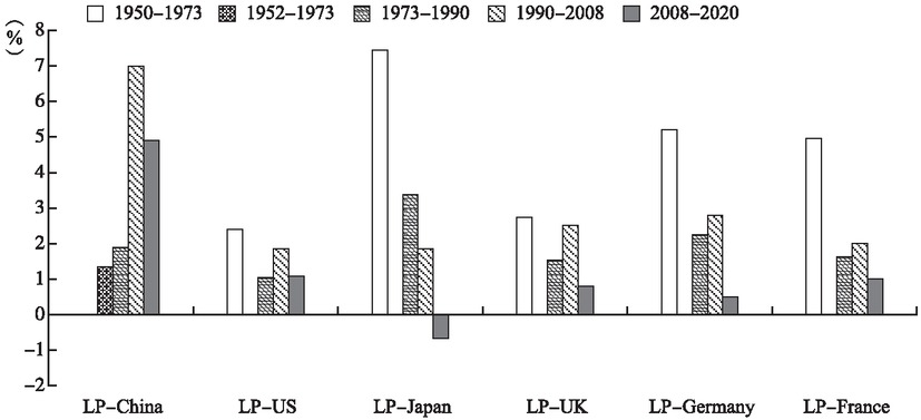
LP Changes in Major Countries
Source: Calculation based on PWT100 data.
LP Changes in Major Countries
| LP−China | LP−US | LP−Japan | LP−UK | LP−Germany | LP−France | |
|---|---|---|---|---|---|---|
| 1952−1973 | 1.38% | 2.33% | 7.35% | 2.93% | 4.86% | 5.04% |
| 1973−1990 | 1.91% | 1.05% | 3.40% | 1.55% | 2.28% | 1.61% |
| 1990−2008 | 6.96% | 1.88% | 1.86% | 2.54% | 2.82% | 2.01% |
| 2008−2020 | 4.91% | 1.12% | −0.64% | 0.85% | 0.52% | 0.98% |
Source: Calculation based on PWT100 data.
According to the changes with TFP and LP, the world economy entered an upward cycle in the 1990s after the “stagflation”, but then started a downward cycle after the financial crisis in 2008. Given the lasting influence of COVID-19 and Russia-Ukraine conflict, the possibility of another “stagflation” for the world economy cannot be ruled out.
3.2 Inflation, Monetary Policy and Fiscal Policy
In the efforts to govern the “stagflation” in the 1970s, policies against inflation were most prominent and also most effective. Compared with economic growth and unemployment, inflation was the first to be kept in control.
Monetary policy is generally believed the most effective approach for governing inflation. In particular, the classical theory and literature proposed “one goal, one tool”, not only making stabilization of general price level the critical basis for effective execution of monetary policy, but improving the policy predictability and transparency. As practice deepened, regulation capacity of monetary policy for general price level in broad sense is constantly questioned. Whether monetary policy alone could determine general price level or not has attracted extensive attention. Given the increasingly stronger influence of asset price on general price level, validity of monetary policy and tools is worth noticing. If blended with unemployment and economic recession, use of monetary policy would curb inflation, but also intensify the recession and unemployment at the same time.
In the 1990s, the fiscal theory of the price level (FTPL) emerged, calling for attention to the actual role and influence of fiscal policy in the formation and regulation of inflation. The theory was first proposed by Sargent and Wallace (1981). It is believed that if the power of fiscal sector is stronger than the monetary sector, the fiscal deficit that is out of effective control would force the monetary sector to keep issuing money for financing, until interest rate of bonds exceed economic growth, when the monetary sector is unable to continue with money supply for financing, which inevitably lead to inflation. The theory is called “some unpleasant monetarist arithmetic”. According to Leeper (1991), in the case of combined prudent monetary policy and proactive fiscal policy in macroeconomic operation, inflation is mainly determined by fiscal policy; in the case of proactive monetary policy and proactive fiscal policy, inflation may go out of control. Up to this point, it is generally believed inflation is jointly decided by monetary and fiscal policies and its governance should take them both into comprehensive consideration. Research afterwards proposed that even without the effect of monetary policy, fiscal policy alone could determine the general price level (Woodford, 1995,1996 and 2001; Cochrane, 2005). This reflects the existence of “wealth effect” of government revenue and expenditure. If macro-policies are in a “non-Ricardian regime”, or in another word basic government surplus is an exogenous variable, bonds issued by government would not drive consumers to lower current consumption out of expectations for future tax rise, but instead spur them for consumption because of the more bonds in hand. At the equilibrium level, when product market and government budget reach a status of clearing at the same time, price level is determined by fiscal policy alone.
Research on the fiscal theory of the price level started late in China, but it is of high academic and realistic value because of the unique fiscal and monetary relations in China. Gong and Zou (2002) believed price level was determined by the equation of actual value of government bonds and fiscal surplus of government. On the one hand, China’s fiscal decentralization and county-level development competition give rise to the close ties between banks and local government in economic development, i.e. the role of local commercial banks as second finance. In such circumstances, to go with credit easing for the purpose of fiscal financing and economic development would probably affect the trend of general price level (Qian and Roland, 1998; Bennett and Dixon, 2001). On the other hand, local government in developing local economy tends to input excessive factors of production, inevitably leading to the rapid rise of local general price level (Xu et al., 2007).
Zhao and Zhou (2009) used categorical data of Chinese provincial fiscal expenditure in 1992–2006 to study the correlation between local government’s competition in fiscal expenditure and inflation. Empirical analysis was conducted from the perspectives of fiscal expenditure’s “wealth effect”, “seigniorage effect”, “production effect” and “internal demand effect”. It found the fiscal revenue centralization of central government weakened the impact of inter-government competition in fiscal expenditure on inflation, but its expenditure centralization intensified the impact. Because of the “production effect” and “internal demand effect” of fiscal expenditure, the expenditure competition caused local inflation to drop in the future. Fiscal expenditure and inflation also featured reverse causality because local government would reversely adjust local government expenditure according to price levels in the past. Jia et al. (2014) estimated the reaction function of fiscal and monetary policies and on such basis identified the policies’ systemic reaction to output, inflation, government debts, real estate price and real exchange rate volatility.
The fiscal theory of the price level originates from the theory of rise of states and the evolution of right to issue money. Early states in monopoly of money issuance made net income of coining money in the way of seigniorage by reducing quality of coined money and lowering the weight. The privilege of coining money was a necessary path to earnings and also the origin of inflation at the early stage, which was the earliest connections between fiscal revenue and inflation. Under the system of paper money standard, the meaning of seigniorage and the causes of inflation both changed dramatically. In modern western economic theories, discussions of seigniorage are often associated with monetization of fiscal deficit. When government issues more money to make up the fiscal deficit, the price level rises and money holders suffere loss, but government has higher earnings. The earnings are derived from legitimate government’s monopoly of money issuance through central bank, highly similar to feudal seigniors’ access to seigniorage through monopoly in the sense that they both work at the cost of interests of money holders. This is why the seigniorage collected by government at this time is also called “inflation tax” (Blanchard, 2005).
With the development of economic globalization, research has expanded to the whole world. The New Palgrave: A Dictionary of Economics particularly mentioned the social returns in the form of seigniorage coming from use of special drawing rights (SDR) or US dollars and other international currencies in substitution of gold, i.e. the direct correlation between changes of international general price level and international position and domestic policies of countries of importance in the world economy. Meanwhile, as modern monetary theory and the study develope, connections between monetary and fiscal policies and inflation as well as the influencing mechanisms are becoming increasingly complicated. For instance, the Bank for International Settlements (2003) defined seigniorage as a central bank’s profits from its monopoly of money issuance and equated it to the product of the central bank’s non-interest liabilities and interest rate of government long-term bonds (LTBR).
The influence of fiscal policy on inflation requires high regulation in the future academic research and policy making. Different from the view of the classical inflation theory that believes money supply endogenous, finance-originated money supply is exogenous money, which is more likely to trigger inflation and other problems and makes it harder to draw up macro-policies.
References
Breitenfellner, A., & Cuaresma, J. (2008). Crude Oil Prices and the Euro-Dollar Exchange Rate: A Forecasting Exercise. Working Papers in Economies and Statistics. Innsbruck: University of Innsbruck.Search in Google Scholar
Carruth, A., Hooker, M., & Oswald, A. (1998). Unemployment Equilibria and Input Prices: Theory and Evidence from the United States. Review of Economics and Statistics, 80, 621–628.10.1162/003465398557708Search in Google Scholar
Cheng, K. (2008). Dollar Depreciation and Commodity Prices. in IMF. (eds.) World Economic Outlook. Washington D.C.: International Monetary Fund, 72–75.Search in Google Scholar
Gordon, R. (2016). The Rise and Fall of American Growth: The U.S. Standard of Living Since the Civil War. Princeton, NJ: Princeton University Press.10.1515/9781400873302Search in Google Scholar
Grubb, D., Jackman, R., & Layard, R. (1982). Causes of the Current Stagflation. The Review of Economic Studies. (Special Issue on Unemployment), 49(5), 707–730.10.2307/2297186Search in Google Scholar
Helliwell, J. (1988). Comparative Macroeconomics of Stagflation. Journal of Economic Literature, 26(1), 1–28.Search in Google Scholar
Helliwell, J. (1988). Comparative Macroeconomics of Stagflation. Journal of Economic Literature, 26(1), 1–28.Search in Google Scholar
Hooker, M. (1996). What Happened to the Oil Price-Macroeconomy Relationship? Journal of Monetary Economics, 38, 195–213.10.1016/S0304-3932(96)01281-0Search in Google Scholar
Jorgenson, D., & Wilcoxen, P. (1990). Environmental Regulation and U.S. Economic Growth. The RAND Journal of Economics, 21(2), 314–340.10.2307/2555426Search in Google Scholar
Joshi, S., Krishnan, R., & Lave, L. (2001). Estimating the Hidden Costs of Environmental Regulation. The Accounting Review, 76(2), 171–198.10.2308/accr.2001.76.2.171Search in Google Scholar
Keane, M., & Prasad, E. (1996). The Employment and Wage Effects of Oil Price Changes: A Sectoral Analysis. Review of Economics and Statistics, 78, 389–400.10.2307/2109786Search in Google Scholar
Krugman, P., (1983). Oil and the Dollar. In Bahandari, J., & Putnam, B. (eds.) Economic Interdependence and Flexible Exchange Rates. Cambridge, MA: MIT Press.Search in Google Scholar
Li, D. (2012). Policy Practice and Inspirations of Reagoneconomics. Public Finance Research (Caizheng Yanjiu), 1, 79–81.Search in Google Scholar
Lizardo, R., & Mollick, A. (2009). Oil Price Fluctuations and U.S. Dollar Exchange Rates. Energy Economics. doi: 10.1016/j.eneco.2009.10.005.10.1016/j.eneco.2009.10.005.Search in Google Scholar
Maddison, A. (2003). The World Economy: Historical Statistics. Paris: OECD, 260–263.10.1787/9789264104143-enSearch in Google Scholar
Olson, M. (1982). Stagflation and the Political Economy of the Decline in Productivity. American Economic Review, 72(2), 143–148.Search in Google Scholar
Phelps, E. (1967). Philips Curves, Expectations of Inflation and Optimal Employment over Time. Economica, 34, 254–281.10.2307/2552025Search in Google Scholar
Phelps, E. (1994). Structural Slumps. Cambridge, MA: Harvard University Press.Search in Google Scholar
© 2023 Zhenxia Wang, Published by DeGruyter
This work is licensed under the Creative Commons Attribution 4.0 International License.
Articles in the same Issue
- Frontmater
- Structural Evolution of RMB Exchange Rate Reform: Historical Review, Experience and Prospect
- A Study of Coordinating China’s Two-Pillar Regulatory Policy under the Shock of the Fed’s Interest Rate Hike—From the Perspective of “Stable Growth” and “Risk Prevention”
- The “Stagflation” Risk and Policy Control: Causes, Governance and Inspirations
- Robot Application and Adjustment of Export Product Scope: Can We Have Both Efficiency and Quality?
- The Effect of “Pressure-Type” Fiscal Incentives on Industrial Restructuring in China
- Convergence Analysis of Village Collective Economy Based on a Long-Term (1978–2018) Observation of 40 Villages in the Suburbs of Beijing