A novel MOSnet model for multi-object segmentation of medical images in micro-computed tomography
-
Kunpeng Wang
 ,
Yueyue Xiao
,
Yueyue Xiao

Abstract
Objectives
Micro-computed tomography (Micro-CT) is renowned for its high resolution, holding a pivotal role in advancing medical science research. However, compared to CT medical imaging datasets, there are fewer publicly available Micro-CT datasets, especially those annotated for multiple objects, leading to segmentation models with limited generalization abilities.
Methods
In order to improve the accuracy of multi-organ segmentation in Micro-CT, we developed a novel segmentation model called MOSnet which can utilize annotations from different datasets to enhance the whole segmentation performance. The proposed MOSnet includes a control module coupled with a reconstruction block that forms a multi-task structure, effectively addressing the absence of complete annotations.
Results
Experiments on 85 contrast-enhanced micro-CTscans and 140 native micro-CTscans for mice demonstrate that MOSnet is superior to the most of advanced segmentation networks. Compared to the best results of ResUnet, Unet3+, DAVnet3+ and AIMOS, our method improved dice similarity coefficient by 4.1 and 2.4 %, increased jaccard similarity coefficient by 4.1 and 3.1 %, and reduced HD95 by 16.3 and 19.3 % on the two datasets respectively at least.
Conclusions
Our proposed model proves to be a robust and effective method for multi-organ segmentation in micro-CT, especially in situations where comprehensive annotations are lacking within a dataset.
Introduction
Micro-computed tomography (Micro-CT) stands out as a prevalent imaging technique in preclinical research, offering detailed insights and variations within inner structures at high resolution [1], 2]. Therefore, Micro-CT plays an important role in small animal model imaging due to its notable repeatability and reliability [3], [4], [5]. Through Micro-CT, researchers can meticulously observe the anatomical details of internal structures within animal models, including bones, organs and tissues [6] and gather extensive anatomical and physiological data, furnishing valuable insights for preclinical research and facilitating advancements in drug development and treatment modalities [7]. A thorough understanding and characterization of animal models are considered crucial for enhancing the reproducibility of applications in humans. In various research fields, spanning from cancer pathology [8], 9] to radiation research [10], medication delivery [11], and nanoparticle absorption [12], analyzing acquired animal imaging data quantitatively and comparatively necessitates the segmentation of different objects.
Among animal models in Micro-CT research, mice are the most commonly used organisms in studying diseases that occur in humans [13]. Therefore, segmentation of mouse organs in Micro-CT takes a critical role in data analyses across numerous biomedical researches [14], [15], [16]. The traditional method is conducted by manually outlining object contours of a volumetric scan slice by slice. However, this process demands a significant attention to anatomical and imaging details, making it highly repetitive and time-consuming. Even for experts, manual segmentation is a challenging task susceptible to human errors and biases, particularly in those imaging modalities with low contrast, which may adversely affect the accuracy and objectiveness of obtained results [17]. Consequently, a pressing demand exists for automated segmentation of multiple organs, a field that has garnered significant attention and research efforts over the course of decades [18]. The predominant conventional methods for mouse organ segmentation involve the utilization of some anatomical atlases that can be applied to the scans through elastic deformation, thereby making assumptions about shapes and sizes [19]. Additionally, other approaches encompass techniques rooted in traditional machine learning [20], such as support vector machines [21] and random forests [22]. Unfortunately, despite their widespread usage, these methods often fall short of achieving satisfactory quality.
In recent years, there has been a growing utilization of deep learning techniques for mouse organ segmentation. Several studies suggest that segmentation based on deep learning produces more accurate and consistent results compared to atlas-based methods [23]. Wang et al. [24] proposed a two-stage deep supervised network (TS-DSN) to delineate organs in the mouse torso. The network employs a two-stage workflow design, initially predicting rough regions for multiple organs and subsequently refining the accuracy of local regions for each organ. Schoppe et al. [25] introduced a deep learning pipeline for segmenting organs of mice, called AIMOS (AI-based Mouse Organ Segmentation). However, the scarcity of open-source datasets for mouse organs and the limited annotations for partial complex organs persist as significant challenges, hindering progress in multi-organ segmentation tasks. A single dataset may not encompass all required masks, and disparities in imaging parameters across different datasets are common. Simply mixing different datasets to train a model may affect the accuracy of segmentation algorithms. Dmitriev [26] proposed a conditional convolutional network using multiple partially annotated datasets, which performs multi-target segmentation by adding conditional encoding to the down-sampling layer. Given the diversity of targets, the aforementioned models are simplistic and fail to sufficiently disentangle features for each individual organ.
In addressing the issues such as insufficient decoupling of features for multiple organs in the existing algorithms, we proposed a novel MOSnet model in this work. The proposed MOSnet extracts features from both contrast-enhanced Micro-CT and non-enhanced Micro-CT, facilitating a dual integration to mitigate shortcomings inherent in each dataset which enhances the segmentation of mice organs. With a multi-task structure, it generates segmentation probability maps and reconstruction maps, providing complements to adjust the major segmentation training process. Experimental results in this study indicated that our proposed MOSnet achieved significant improvements, demonstrating its wide application prospects in multi-organ segmentation tasks.
Methodology
The architecture of our proposed MOSnet model is illustrated in Figure 1. It mainly consists of a shared encoder, a segmentation decoder and a reconstruction decoder. The segmentation decoder contains a control module which utilizes distinct conditional encodings for different dataset annotations to undergo joint training. The reconstruction decoder is designed to establish a multi-task framework aimed at aiding in the primary segmentation.
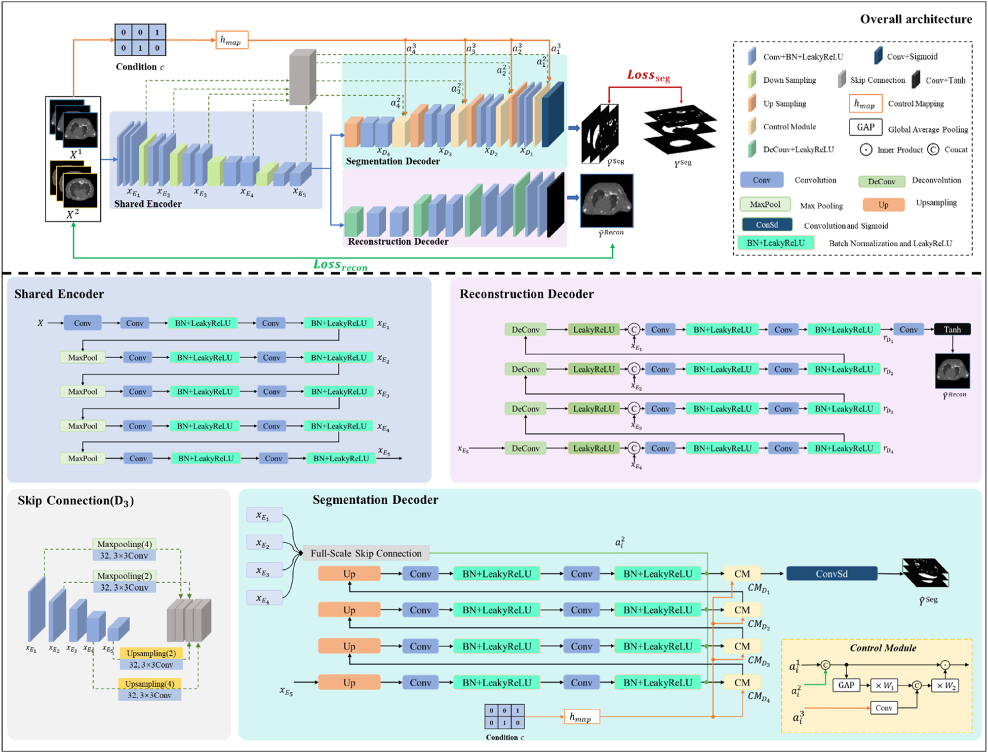
The architecture of our proposed MOSnet model.
Consider a set
The shared encoder, illustrated in Figure 1, consists of several convolutional and pooling layers, gradually reducing the dimensions of the input image and extracting features. Formally, the encoder includes double-convolution units and the output
where Conv3(·) represents a 3 × 3 convolution operation in the encoder layer E i , with a stride of 1 and padding of 1, BL(·) denotes batch normalization followed by a LeakyReLU activation function, while MaxPool(·) refers to max pooling. The shared encoder enables the model to extract a set of shared representation features, reducing the overall model parameters.
The segmentation decoder generates results in different channels through a series of up-sampling operations, with each channel containing a probability map for a specific organ. Because it is difficult to obtain a dataset with complete target annotations, and the information within a single dataset is not adequate to train a comprehensive model capable of segmenting all targets, we introduced an explicit control module between the shared encoder and the segmentation decoder to integrate features inherent in different datasets. Unlike classical approaches that train a separate model for each class, the proposed method employs distinct conditional codes for different dataset annotations, guiding the model to perform target segmentation on similar objects with labels from various datasets. In contrast to implicit control through loss functions, the explicit control module adds conditional feedback on top of the loss function, enhancing the model’s perceptual capabilities towards data. Additionally, the introduced control module in the segmentation decoder incorporates the influence of the controlled object itself during the conditional encoding adjustment, aiding in the model’s ability to decouple features of multiple organs.
As shown in Figure 1, the input of the control module
where
where hmap(·) is a hash function for a pre-defined lookup table and c represents the condition code according to the dataset’s class. The hash function hmap(c) is designed to unify heterogeneous dataset annotations into a shared embedding space. The input is a categorical label c and the output is a fixed-size embedding vector. A unique index is assigned each unique label and a pre-defined lookup table initialized with random values. During training, the table is updated via backpropagaion to encode dataset-specific characteristics. Therefore, the control module’s output of the layer D
i
with inputs
where Conv(·) is a 1 × 1 convolutional operation followed with a LeakyReLU, φgap(·) is a global average pooling, and
The reconstruction decoder utilizes the feature information extracted by the shared encoder to generate an image that will be compared with the original input image, so as to make the feature information more complete. As illustrated in Figure 1, the reconstruction decoder consists of deconvolution, feature concatenation, double convolution, batch normalization, and activation functions.
The output
where Conv3(·) represents a 3 × 3 convolution operation with a stride of 1 and padding of 1, BL(·) denotes batch normalization followed by a LeakyReLU activation function, Cat(·) denotes feature concatenation, and DeConv(·) represents a deconvolution with a 3 × 3 kernel, stride of 2, and padding of 1.
The reconstruction decoder assists the shared encoder in extracting semantic features from deeper layers and higher-resolution attributes from shallower layers, which are used in the segmentation decoder to generate higher-precision segmentation probability maps. All of them together form a multi-task structure, where different tasks mutually influence each other through shared parameters, thereby enhancing overall performance and improving the results of the primary task.
The input image passed through MOSnet has two outputs: a segmentation result
where for each class i, α
i
= {0,1} specifies the presence or not of the binary mask in the batch; β
i
specifies its impact on the total loss, which is determined by the ratio of the number of different labeled samples so as to ensure that the network can accurately segment each organ;
where X is the original image and
where λ is the weight factor of the reconstruction loss.
Experiments and results
Datasets
Due to the widespread use of mouse model in Micro-CT research, in this study, two datasets were utilized to evaluate the segmentation accuracy of the proposed MOSnet: one native mouse Micro-CT dataset without any contrast agents and one contrast-enhanced mouse Micro-CT dataset with a contrast agent injected. All of them were obtained from Nature Scientific Data [27].
The native dataset consists of 140 whole-body scans from 20 mice by a preclinical Micro-CT. In this dataset, the field of view was 40.32 × 28.84 × 55.44 mm, and the voxel size was 0.28 × 0.28 × 0.28 mm [27]. The native dataset has the ground truth of these organs: heart, lungs, liver, kidneys, spleen, bladder and intestine.
The contrast-enhanced dataset involves 85 whole-body scans from 10 mice by a preclinical Micro-CT. Before the first scan, the contrast agent was intravenously injected, which is able to enhance the contrast of spleen and liver in Micro-CT. In the contrast-enhanced dataset, the field of view was 43.12 × 33.88 × 67.76 mm, and the voxel size was 0.28 × 0.28 × 0.28 mm [27]. This dataset has the ground truth of these organs: heart, lungs, liver, kidneys, spleen, bladder, intestine, stomach and bone.
Due to the different field of view and different size between the two datasets, 2D segmentation is more suitable than 3D segmentation [28]. Before the training, we preprocessed the data by adjusting the window width to 1000 HU and the window level to 400 HU for each slice, followed by normalization to a range of 0–1 to mitigate relative numerical discrepancies across the data. In order to achieve multi-organ segmentation, we trained both datasets in the same network simultaneously. A total of 50,591 slices were randomly divided at a ratio of 9:1 for training and validation respectively.
Evaluation metrics
In this study, we evaluated the performance of the proposed MOSnet quantitatively through three widely recognized evaluation metrics: dice similarity coefficient (DSC), jaccard similarity coefficient (JSC), and 95%hausdorff distance (HD95). Their calculation formulas are as follows:
where
Implementation
In this study, we chose the Adam optimizer algorithm, setting 0.001 as the initial learning rate for updating the parameters of the network and a scheduler for updating the learning rate. The training is through 100 epochs using a batch-size of 16 images. All experiments were executed using PyTorch on a machine equipped with a GPU of NVIDIA 2080Ti.
Experiment results
For illustrating the efficacy of the proposed MOSnet, we compared its prediction results of the two datasets with those of four excellent segmentation networks: ResUnet [29], Unet3+ [30], DAVnet3+ [31], and AIMOS [25]. To maintain fairness in comparison, we chose identical preprocessing for these networks and refrained from postprocessing. Also, their batch-sizes, epochs, optimizers and schedulers are consistent for all networks.
The results of qualitative comparison are shown in Figure 2. As evident from these figures, despite these networks achieving high accuracy, the results of MOSnet are more consistent with the ground truth than the other networks. For the native dataset, our method accurately delineates the target regions of the liver, spleen, bladder, and intestine, exhibiting precise boundaries. Similarly, for the contrast-enhanced dataset, the stomach region is accurately portrayed with meticulous contours by our model. Although MOSnet outperforms other networks, there may be some areas where the segmentation results are not entirely satisfactory, particularly when dealing with lungs of the native dataset. Nevertheless, it consistently demonstrates a lower number of segmentation errors compared to other networks.
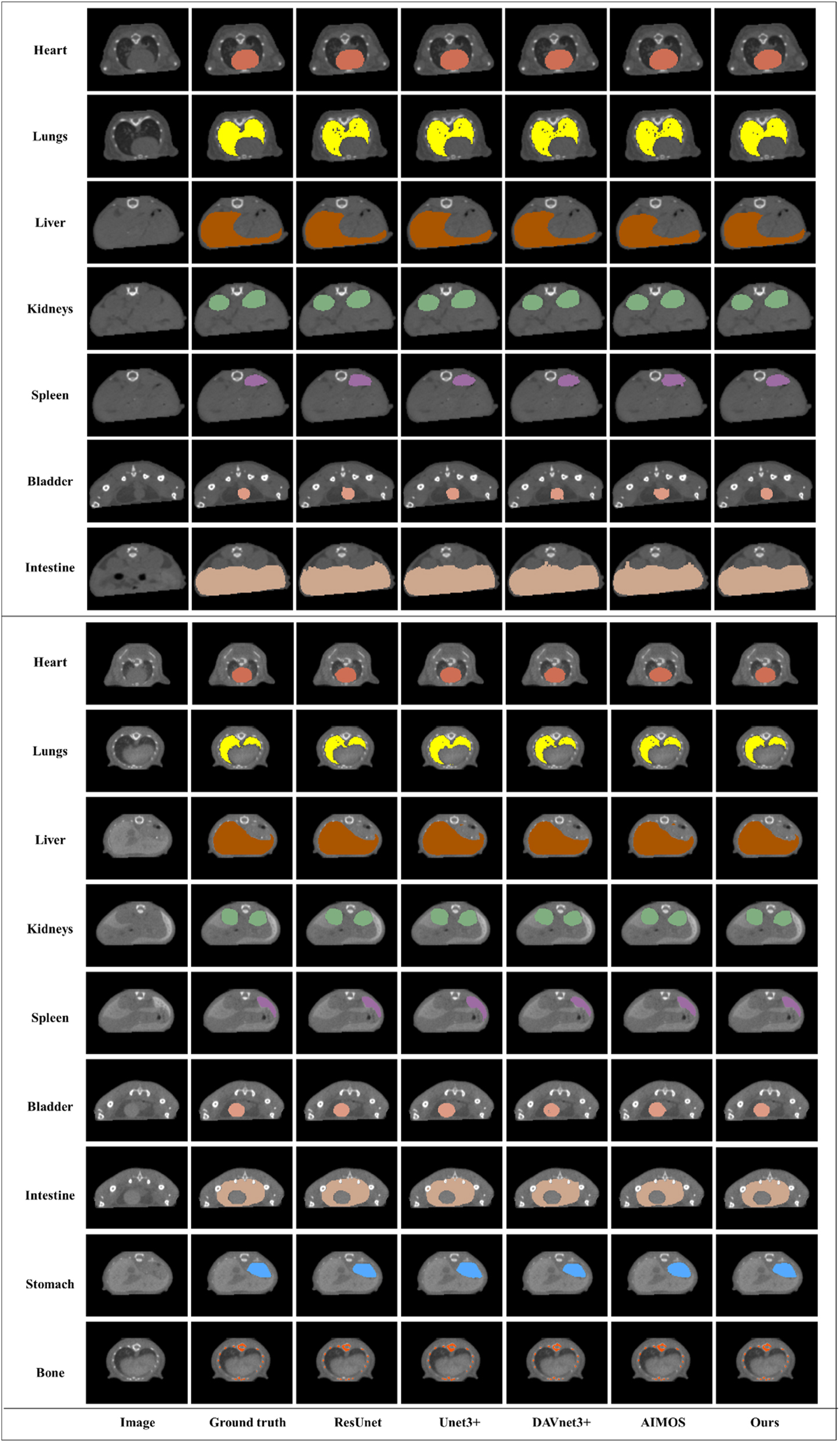
Segmentation results of the five networks for the native dataset (UP) and the contrast-enhanced dataset (Down).
Tables 1 and 2 present the quantitative results of all methods evaluated on the two datasets. By analyzing the experimental data, the results of the proposed MOSnet exhibit its superior performance to ResUnet, Unet3+, DAVnet3+, and AIMOS. It can be observed that MOSnet, compared to the best-performing network, evenly improves DSC by 4.1 and 2.4 %, increased JSC by 4.1 and 3.1 %, simultaneously reducing HD95 by 16.3 and 19.3 % on the two datasets respectively. From the perspective of the segmentation results of each organ, the difficulty of segmenting intestine is the biggest, but our model still achieved best, particularly improving the DSC value by 0.078, 0.053, 0.014, 0.023 and 0.039, 0.064, 0.022, 0.009. This indicates that in the multi-organ segmentation task, MOSnet effectively enhances the accuracy especially in complex regions when completing the segmentation of various targets.
Experimental results of the five networks for the native dataset.
| Evaluation | Methods | Heart | Lungs | Liver | Kidneys | Spleen | Bladder | Intestine |
|---|---|---|---|---|---|---|---|---|
| DSC↑ | ResUnet | 0.921 (0.064) |
0.913 (0.071) |
0.888 (0.094) |
0.904 (0.078) |
0.928 (0.056) |
0.918 (0.087) |
0.829 (0.096) |
| Unet3+ | 0.948 (0.066) |
0.921 (0.084) |
0.896 (0.090) |
0.919 (0.080) |
0.934 (0.073) |
0.923 (0.084) |
0.854 (0.131) |
|
| DAVnet3+ | 0.941 (0.045) |
0.919 (0.057) |
0.907 (0.067) |
0.901 (0.059) |
0.913 (0.061) |
0.920 (0.049) |
0.893 (0.085) |
|
| AIMOS | 0.923 (0.050) |
0.927 (0.077) |
0.887 (0.067) |
0.894 (0.075) |
0.905 (0.122) |
0.927 (0.066) |
0.884 (0.088) |
|
| Ours |
0.979
(0.036) |
0.959
(0.059) |
0.925
(0.061) |
0.958
(0.052) |
0.962
(0.051) |
0.954
(0.044) |
0.907
(0.076) |
|
| JSC↑ | ResUnet | 0.923 (0.066) |
0.936 (0.072) |
0.873 (0.098) |
0.891 (0.081) |
0.909 (0.061) |
0.902 (0.088) |
0.844 (0.101) |
| Unet3+ | 0.939 (0.068) |
0.914 (0.085) |
0.880 (0.094) |
0.905 (0.083) |
0.924 (0.078) |
0.916 (0.085) |
0.829 (0.132) |
|
| DAVnet3+ | 0.923 (0.049) |
0.919 (0.059) |
0.884 (0.072) |
0.906 (0.062) |
0.914 (0.067) |
0.912 (0.053) |
0.868 (0.091) |
|
| AIMOS | 0.947 (0.063) |
0.867 (0.150) |
0.895 (0.088) |
0.892 (0.090) |
0.887 (0.097) |
0.915 (0.086) |
0.866 (0.091) |
|
| Ours |
0.971
(0.040) |
0.951
(0.060) |
0.930
(0.067) |
0.944
(0.058) |
0.953
(0.058) |
0.958
(0.048) |
0.882
(0.084) |
|
| HD95↓ | ResUnet | 2.023 (0.393) |
1.235 (0.525) |
6.908 (2.217) |
5.221 (2.871) |
2.698
(0.526) |
2.864 (1.165) |
8.068 (2.388) |
| Unet3+ | 2.254 (0.512) |
1.278 (0.537) |
7.247 (2.392) |
5.932 (3.227) |
3.488 (0.686) |
2.898 (1.056) |
8.573 (2.378) |
|
| DAVnet3+ | 2.316 (0.496) |
1.322 (0.496) |
7.637 (2.837) |
5.778 (2.675) |
3.580 (0.756) |
2.935 (0.812) |
8.779 (2.496) |
|
| AIMOS | 2.206 (0.611) |
2.048 (1.015) |
7.237 (2.340) |
5.539 (2.971) |
4.380 (0.722) |
3.384 (1.204) |
8.762 (2.411) |
|
| Ours |
1.942
(0.442) |
1.206
(0.534) |
6.843
(2.405) |
4.311
(2.367) |
2.835 (0.483) |
2.301
(0.627) |
7.826
(2.316) |
-
The mean and standard error are presented in this table. The bold values indicate the best performance for each metric.
Experimental results of the five networks for the contrast-enhanced dataset.
| Evaluation | Methods | Heart | Lungs | Liver | Kidneys | Spleen | Bladder | Intestine | Stomach | Bone |
|---|---|---|---|---|---|---|---|---|---|---|
| DSC↑ | ResUnet | 0.903 (0.067) |
0.869 (0.072) |
0.903 (0.070) |
0.888 (0.079) |
0.831 (0.077) |
0.907 (0.065) |
0.797 (0.107) |
0.860 (0.082) |
0.860 (0.014) |
| Unet3+ | 0.912 (0.086) |
0.899 (0.109) |
0.898 (0.123) |
0.847 (0.106) |
0.851 (0.108) |
0.927 (0.133) |
0.772 (0.133) |
0.893 (0.120) |
0.894 (0.017) |
|
| DAVnet3+ | 0.909 (0.070) |
0.921 (0.076) |
0.906 (0.069) |
0.891 (0.077) |
0.906 (0.073) |
0.920 (0.070) |
0.814 (0.101) |
0.889 (0.085) |
0.919 (0.013) |
|
| AIMOS | 0.925 (0.047) |
0.935 (0.065) |
0.892 (0.068) |
0.878 (0.085) |
0.899 (0.066) |
0.916 (0.088) |
0.827 (0.052) |
0.879 (0.041) |
0.826 (0.055) |
|
| Ours |
0.930
(0.076) |
0.942
(0.063) |
0.937
(0.082) |
0.929
(0.067) |
0.935
(0.075) |
0.936
(0.074) |
0.836
(0.106) |
0.926
(0.078) |
0.929
(0.013) |
|
| JSC↑ | ResUnet | 0.911 (0.070) |
0.893 (0.076) |
0.909
(0.075) |
0.816 (0.085) |
0.822 (0.079) |
0.907 (0.069) |
0.750 (0.111) |
0.859 (0.086) |
0.855 (0.022) |
| Unet3+ | 0.911 (0.088) |
0.896 (0.111) |
0.899 (0.124) |
0.885 (0.109) |
0.834 (0.111) |
0.910 (0.134) |
0.743 (0.131) |
0.892 (0.122) |
0.813 (0.027) |
|
| DAVnet3+ | 0.908 (0.073) |
0.903 (0.080) |
0.905 (0.075) |
0.879 (0.083) |
0.876 (0.075) |
0.917 (0.074) |
0.726 (0.106) |
0.885 (0.089) |
0.833 (0.022) |
|
| AIMOS | 0.908 (0.085) |
0.836 (0.133) |
0.878 (0.124) |
0.875 (0.091) |
0.809 (0.145) |
0.920 (0.081) |
0.686 (0.123) |
0.855 (0.109) |
0.817 (0.026) |
|
| Ours |
0.919
(0.079) |
0.925
(0.068) |
0.897 (0.086) |
0.907
(0.074) |
0.927
(0.077) |
0.927
(0.077) |
0.788
(0.111) |
0.916
(0.082) |
0.869
(0.021) |
|
| HD95↓ | ResUnet | 2.992 (0.765) |
1.925 (0.765) |
6.814
(3.003) |
6.038 (2.559) |
2.339 (1.089) |
2.962 (0.774) |
9.373 (3.267) |
5.291
(1.048) |
1.142 (0.516) |
| Unet3+ | 3.059 (0.885) |
3.725 (1.286) |
7.403 (4.688) |
6.532 (2.473) |
3.709 (2.398) |
3.056 (1.149) |
9.199 (3.589) |
6.802 (2.294) |
1.146 (1.086) |
|
| DAVnet3+ | 3.377 (0.831) |
3.490 (1.237) |
7.856 (2.697) |
6.966 (2.496) |
3.728 (2.384) |
3.250 (0.771) |
9.240 (3.002) |
6.253 (1.364) |
1.224 (0.497) |
|
| AIMOS | 3.317 (0.985) |
2.456 (1.318) |
7.911 (3.496) |
6.877 (2.883) |
3.161 (1.899) |
2.657 (0.768) |
10.295 (3.635) |
5.957 (1.266) |
1.907 (1.818) |
|
| Ours |
2.988
(0.774) |
1.897
(0.830) |
7.485 (3.423) |
5.589
(2.270) |
1.462
(0.930) |
2.525
(0.861) |
9.188
(3.178) |
5.876 (1.259) |
1.095
(0.665) |
-
The mean and standard error are presented in this table. The bold values indicate the best performance for each metric.
Additionally, Figure 3 displays several histograms about the three metrics of these five networks. It is obvious that no matter for the native dataset or the contrast-enhanced dataset, our proposed MOSnet has the best results on the multi-organ segmentation with the highest average DSC and JSC, and the lowest average HD95. Although the standard error of MOSnet on the contrast-enhanced dataset is somewhat higher partially compared to other segmentation models, it is exhibited the lowest across almost all organs on the native dataset. This observation suggests that our model possesses greater robustness and stability, especially when dealing with different datasets and multi-organ segmentation.
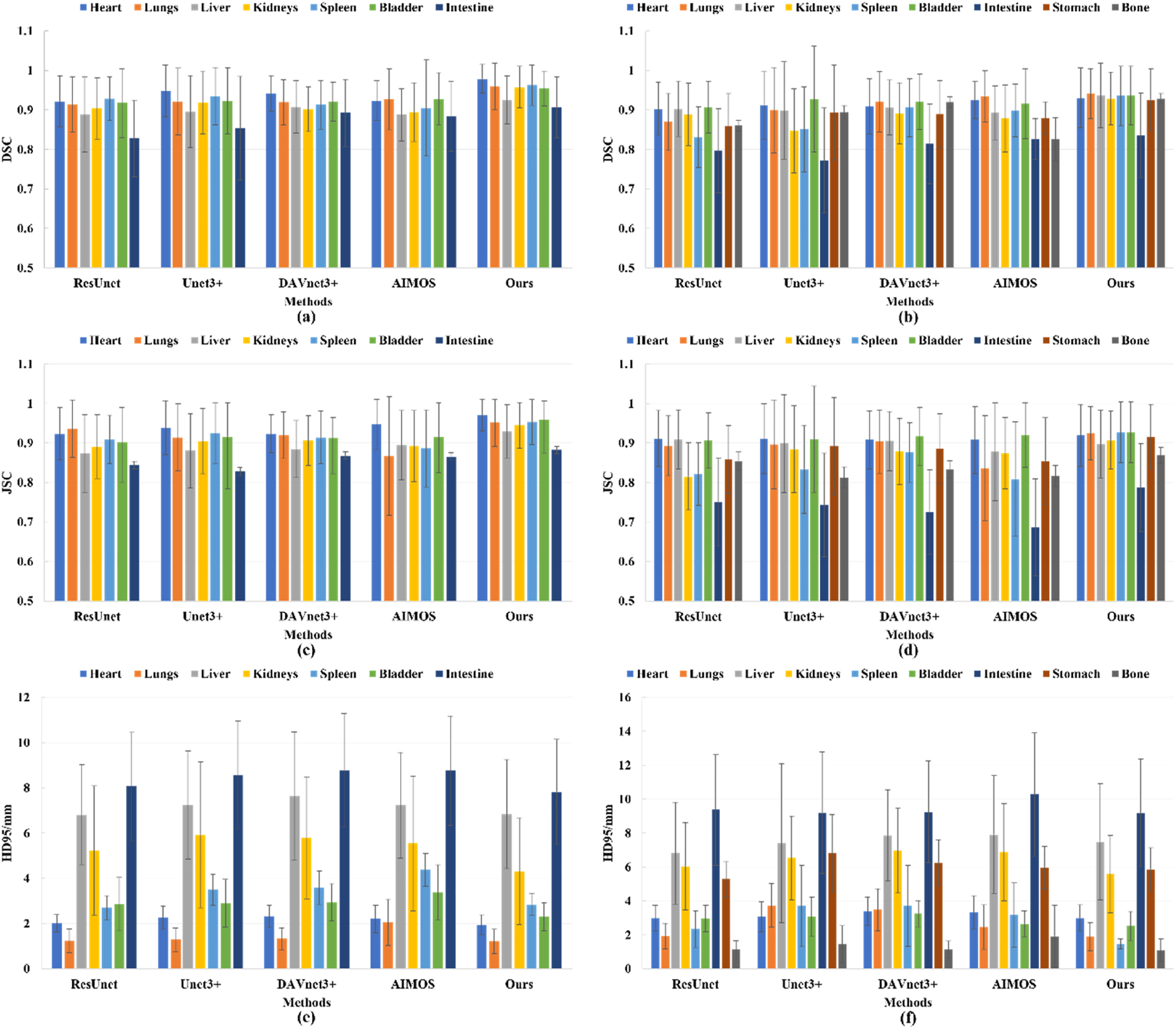
Histograms of DSC, JSC, and HD95 of the networks (The first column represents the native dataset, and the second column represents the contrast-enhanced dataset. The colorful bars are the average values for different organs, and the black lines are the standard errors for the corresponding average values.)
Discussion
This study proposed a method MOSnet for multi-organ segmentation in joint datasets. By exploiting the connections between various datasets and introducing a reconstruction block, the approach achieves accurate segmentation of multiple targets, contributing to addressing complex medical imaging processing tasks.
Advantages of the proposed MOSnet
According to the above results of experiments for segmenting multiple organs, it has been suggested that our proposed MOSnet can accomplish high accuracy with training two datasets simultaneously, which jointly learned features of organs under different parameters. Furthermore, despite the incomplete labeling of the first dataset, the participation of the second dataset through collaborative learning enabled the segmentation of organs unlabeled in the first dataset.
To validate the ability of transfer learning employed by MOSnet, we conducted the following experiment: the labels of the kidneys and bladder in the second dataset were excluded from training and only used to calculate evaluation indicators. The results of this experiment are presented in Table 3 and Figure 4(a). By this way, we aimed to assess the model’s ability to generalize and adapt to untrained data. This experiment served as a rigorous test of MOSnet’s transfer learning capabilities, as it challenged the model to learn and segment organs effectively even without direct supervision from labeled data.
Experimental results of kidneys and bladder.
| Organ | DSC↑ | JSC↑ | HD95↓ |
|---|---|---|---|
| Kidneys | 0.884 (0.094) |
0.855 (0.104) |
6.21 (3.72) |
| Bladder | 0.912 (0.067) |
0.892 (0.071) |
3.16 (0.798) |
-
The mean and standard error are presented in this table.
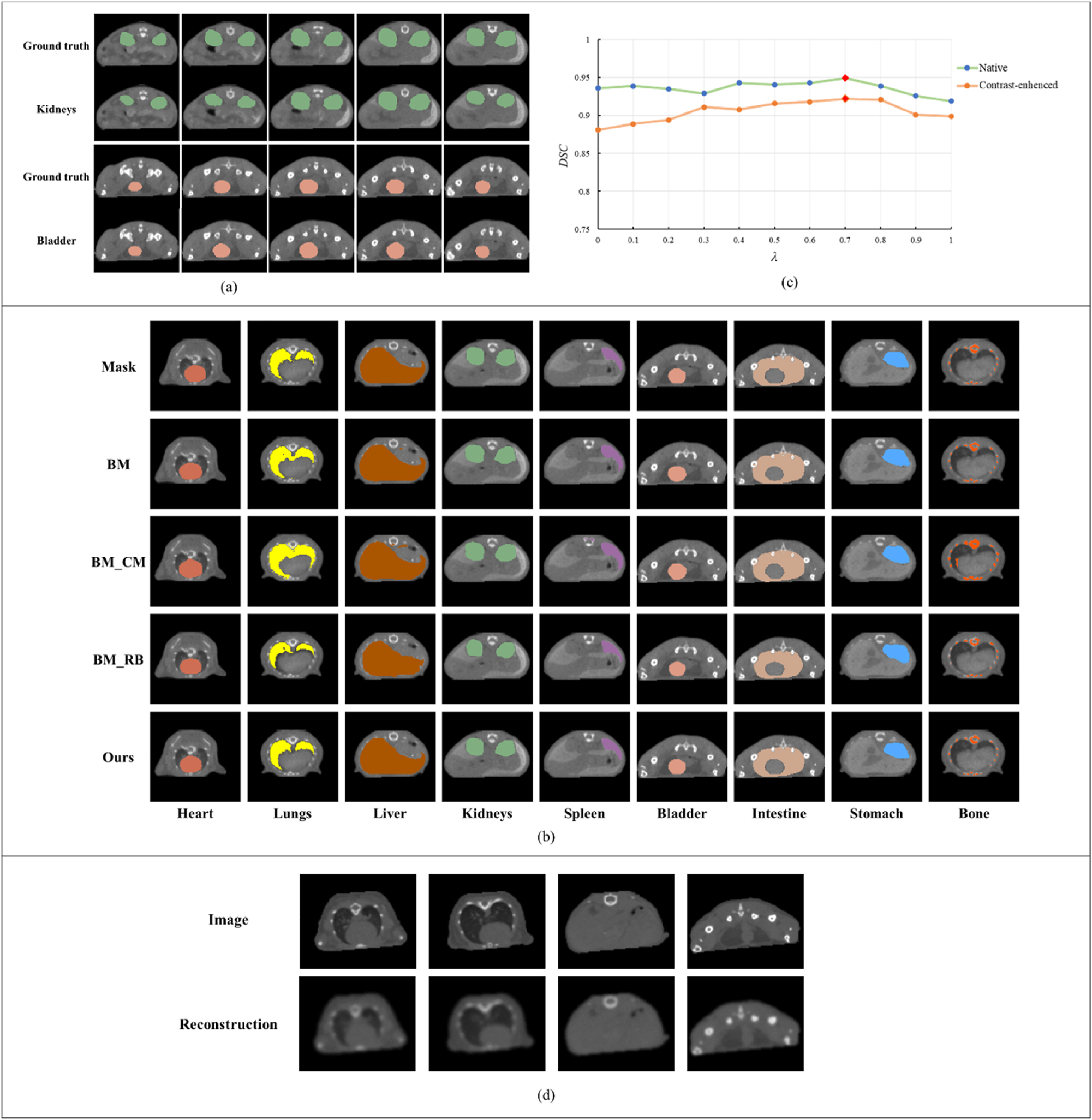
The results of different experiments. (a) The results of kidneys and bladder. (b) Visual results of ablation study. (c) The results under different λ values. (d) The result of the reconstruction decoder.
The results presented in Table 3 and Figure 4(a) demonstrate the model can achieve precise segmentation of target organs by leveraging features learned from other datasets – even when partial organ labels are missing in a single dataset. This further validates the model’s generalization capability and the effectiveness of its transfer learning mechanism.
The results presented in Table 3 demonstrate the model can segment organs accurately enough even in the absence of labeled data, which demonstrated the power of MOSnet in handling various datasets and addressing challenges associated with incomplete annotations. This validates the effectiveness of MOSnet’s transfer learning approach, which leverages knowledge learned from one dataset to enhance the segmentation of organs in another dataset. The experiment highlights the significant potential of MOSnet in real-world scenarios where complete and accurate annotations may not always be available.
This capability was achieved by incorporating a control module and a reconstruction block, and we conducted several systematic experiments to evaluate the efficacy of these modules. The basic model (BM) of MOSnet adopts an end-to-end framework, which includes nested and dense skip connections. Based on BM, a control module and a reconstruction block were added to form the proposed method MOSnet. So, we compared MOSnet to the BM, the basic model with a control module (BM_CM) and the basic model with a reconstruction block (BM_RB) on the validation of the contrast-enhanced dataset.
The ablation study results and statistical significance testing results, shown in Table 4 and Figure 4(b), demonstrate that the BM_CM significantly enhances the performance of multi-organ segmentation compared to the BM. For instance, the stomach’s DSC improves from 0.873 (BM) to 0.903 (BM_CM), and the spleen’s JSC increases from 0.824 (BM) to 0.841 (BM_CM). These improvements indicate that the control module effectively refines the segmentation process by dynamically studying feature representations from different datasets. However, the BM_CM remains susceptible to incomplete segmentation, particularly for organs with ambiguous boundaries, such as the liver and intestine. For example, the liver’s DSC in BM_CM is 0.894, but our model achieves 0.937, a +4.8 % improvement, suggesting that the control module may over-suppress weak signals at the liver’s periphery, leading to information loss. Similarly, the intestine’s DSC in BM_CM is 0.766, significantly lower than the 0.836 in Ours. To address these limitations, a reconstruction block was integrated into the framework, forming a multi-task learning approach that generates reconstruction maps alongside segmentation probability maps. This design enables the model to retain fine anatomical details. It can be clearly seen from the performance of the complete model (our model): Among all organs, our model achieved the highest DSC/JSC value and the lowest HD95 value, and made almost all statistically significant improvements (p<0.05). For instance, the lungs’ HD95 decreases from 3.170 (BM_CM) to 1.897 (Ours), indicating sharper boundary localization, while the spleen’s JSC increases from 0.841 (BM_CM) to 0.927 (Ours), resolving ambiguities with adjacent organs. The reconstruction block enhances performance by preserving high-frequency details and implicitly regularizing the model through input reconstruction, reducing overfitting to noisy annotations.
Results of ablation study for the proposed method.
| Method | Heart | Lungs | Liver | Kidneys | Spleen | Bladder | Intestine | Stomach | Bone | |
|---|---|---|---|---|---|---|---|---|---|---|
| DSC↑ | BM | 0.902 | 0.894 | 0.888 | 0.857 | 0.831 | 0.907 | 0.792 | 0.873 | 0.884 |
| BM_CM | 0.914 | 0.914 | 0.894 | 0.869 | 0.860 | 0.916 | 0.766 | 0.903 | 0.899 | |
| BM_RB | 0.906 | 0.911 | 0.899 | 0.867 | 0.861 | 0.912 | 0.732 | 0.912 | 0.899 | |
| Ours | 0.930 | 0.942 | 0.937 | 0.929 | 0.935 | 0.936 | 0.836 | 0.926 | 0.929 | |
| p | Ours vs. BM | ✓ | ✓ | ✓ | ✓ | ✓ | ✓ | ✓ | ✓ | ✓ |
| Ours vs. BM_CM | ✓ | ✓ | ✓ | ✓ | ✓ | ✓ | ✓ | ✓ | ✓ | |
| Ours vs. BM_RB | ✓ | ✓ | ✓ | ✓ | ✓ | ✓ | ✓ | ✓ | ✓ | |
| JSC ↑ | BM | 0.851 | 0.876 | 0.853 | 0.861 | 0.824 | 0.907 | 0.743 | 0.872 | 0.823 |
| BM_CM | 0.899 | 0.903 | 0.882 | 0.895 | 0.841 | 0.916 | 0.755 | 0.899 | 0.841 | |
| BM_RB | 0.895 | 0.916 | 0.878 | 0.885 | 0.843 | 0.912 | 0.722 | 0.891 | 0.819 | |
| Ours | 0.919 | 0.925 | 0.897 | 0.907 | 0.927 | 0.927 | 0.788 | 0.916 | 0.869 | |
| p | Ours vs. BM | ✓ | ✓ | ✓ | ✓ | ✓ | ✓ | ✓ | ✓ | ✓ |
| Ours vs. BM_CM | ✓ | ✓ | ✓ | ✓ | ✓ | ✓ | ✓ | ✓ | ✓ | |
| Ours vs. BM_RB | ✓ | 0.053 | ✓ | ✓ | ✓ | ✓ | ✓ | ✓ | ✓ | |
| HD95↓ | BM | 3.349 | 3.425 | 7.903 | 6.812 | 3.921 | 3.056 | 9.488 | 6.792 | 1.216 |
| BM_CM | 3.014 | 3.170 | 7.850 | 5.734 | 3.774 | 3.199 | 9.457 | 5.924 | 1.153 | |
| BM_RB | 3.070 | 4.208 | 8.766 | 6.039 | 3.366 | 2.897 | 9.485 | 6.889 | 1.298 | |
| Ours | 2.988 | 1.897 | 7.485 | 5.589 | 1.462 | 2.525 | 9.188 | 5.876 | 1.095 | |
| p | Ours vs. BM | ✓ | ✓ | ✓ | ✓ | ✓ | ✓ | ✓ | ✓ | ✓ |
| Ours vs. BM_CM | 0.488 | ✓ | ✓ | 0.148 | ✓ | ✓ | 0.056 | ✓ | 0.081 | |
| Ours vs. BM_RB | ✓ | ✓ | ✓ | ✓ | ✓ | ✓ | ✓ | ✓ | ✓ |
-
The p is the significance testing result of Ours vs. other methods, and ✓ means <0.05. The bold values indicate the best performance for each metric.
In Equation (9), the weighting factor λ for the reconstruction task influences both the feature extraction capability of the shared encoder during training and the accuracy of the primary segmentation task. To optimize segmentation performance, we examined the variation in average DSC across all segmented organs under different λ values. As shown in Figure 4(c), when λ=0.7, the model achieves consistently higher DSC values for both datasets compared to other λ values. When λ<0.6, the model becomes overly focused on segmentation, diminishing the self-supervised regularization effect and resulting in marginal degradation in boundary precision. When λ>0.8, the reconstruction loss is overly down-weighted, weakening its role in preventing feature overfitting. This leads to slightly noisier predictions and reduced robustness. At λ=0.7, we observe the most consistent performance across organs and anatomical scales, suggesting it provides an effective trade-off for the tasks and data distribution in our study. Consequently, the proposed model adopts λ=0.7 in its overall loss function.
Moreover, as shown in Figure 4(d), these visualizations demonstrate that our model is able to generate anatomically plausible and structurally consistent reconstructions, indicating that the shared encoder has learned meaningful and semantically rich representations from the input micro-CT, supporting its utility as an auxiliary task.
Limitations and future works
The segmentation of mouse micro-CT scans plays a crucial role in biomedical research, as the accuracy of organ delineation directly affects the quality of s quantitative analysis. Compared to existing methods, our proposed MOSnet achieves superior segmentation performance across two datasets, primarily attributed to the effective design of the control module and reconstruction block. Nevertheless, several limitations warrant further discussion.
Firstly, although MOSnet demonstrates strong overall performance, segmentation accuracy for anatomically complex organs, particularly the spleen and intestines, still requires improvement. These structures often exhibit high variability in shape and intensity, posing challenges for precise boundary delineation. To enhance accuracy, future work will explore 3D adaptation and interpolation strategies that can fully exploit spatial contextual information across adjacent slices, thereby improving inter-slice coherence and structural consistency. Also, recent advances in vision transformers (ViTs) and hybrid transformer-convolutional architectures have demonstrated remarkable performance in medical image segmentation, particularly in capturing long-range dependencies and modeling global context – capabilities that are highly valuable for whole-body, multi-organ segmentation tasks. In ongoing and future work, we are actively exploring the integration of vision transformer architectures into our 3D segmentation framework for mouse micro-CT data. Secondly, as shown in Table 3, the model’s performance exhibits a noticeable decline when evaluated on external datasets, indicating limited generalization under domain shifts. This underscores the need to incorporate more diverse, multi-source datasets in future training. Moreover, preprocessing strategies such as style standardization or domain adaptation techniques will be essential to harmonize variations in imaging protocols, scanner characteristics, and noise profiles, thereby enhancing the model’s robustness and cross-domain applicability. It is important to note that all reported results in this study were obtained without any post-processing to ensure a fair comparison of the intrinsic segmentation performance of the different models. However, in practical clinical deployment, simple and computationally efficient post-processing techniques are commonly employed to refine segmentation. Lastly, while the current architecture is effective, its reliance on the control module and reconstruction block results in relatively high complexity, leading to increased computational cost and longer training times. Our model has 11.4M parameters, comparable to UNet3+ (9.2M). Training on a GPU of NVIDIA 2080Ti, MOSnet takes approximately 24 h on the full dataset, similar to UNet3+ (∼21.5 h) and 1.3× longer than ResUnet (∼18 h). To facilitate broader adoption and potential deployment in resource-constrained settings, we will focus on developing a more lightweight variant of MOSnet, aiming to maintain high performance while significantly improving efficiency. For instance, morphological operations such as closing or small object removal could potentially further improve the final segmentation quality.
In summary, future efforts will concentrate on integrating 3D contextual modeling, enhancing generalization through domain-invariant preprocessing, and designing a more lightweight network architecture – steps critical for advancing MOSnet from a research prototype toward practical application in preclinical imaging.
Conclusions
This study developed a novel MOSnet model combined with a control module and a reconstruction block for segmenting multiple objects in micro-computed tomography images. In comparison to the previous methods, we utilized the control module to extract feature information from multiple datasets for simultaneous training, and incorporated the reconstruction block to form a multi-task model capable of generating both segmentation probability maps and reconstruction maps concurrently to correct each other. When a dataset lacks labels for a particular target, the control module can acquire the capability to segment that target from another dataset containing its labels, effectively addressing the absence of complete annotations. Meanwhile, the introduced reconstruction block uses parameters shared between the reconstruction task and segmentation task to enhance extraction performance of the encoder. Extensive experiments conducted on the native dataset and contrast-enhanced dataset demonstrated that the proposed MOSnet model outperforms other classical segmentation models which mix datasets directly. In the future, we will pay attention to building a more lightweight multi-organ segmentation model.
Funding source: National Natural Science Foundation of China
Award Identifier / Grant number: 12071215
-
Research ethics: Not applicable.
-
Informed consent: Not applicable.
-
Author contributions: All authors have accepted responsibility for the entire content of this manuscript and approved its submission.
-
Use of Large Language Models, AI and Machine Learning Tools: None declared.
-
Conflict of interest: The authors state no conflict of interest.
-
Research funding: This work was supported by the National Natural Science Foundation of China [grant number 12071215].
-
Data availability: The data can be obtained from Nature Scientific Data at https://doi.org/10.1038/sdata.2018.294.
References
1. Rosenhain, S, Magnuska, ZA, Yamoah Grace, G, Wa’el Al, R, Fabian, K, Felix, G, et al.. A preclinical micro-computed tomography database including 3D whole body organ segmentations. Sci Data 2018;5:1–9.Search in Google Scholar
2. Burghardt, AJ, Link, TM, Majumdar, S. High-resolution computed tomography for clinical imaging of bone microarchitecture. Clin Orthop Relat Res 2011;469:2179–93.10.1007/s11999-010-1766-xSearch in Google Scholar PubMed PubMed Central
3. Zhou, X, Takayama, R, Wang, S, Hara, T, Fujita, H. Deep learning of the sectional appearances of 3D CT images for anatomical structure segmentation based on an FCN voting method. Med Phys 2017;44:5221–33.10.1002/mp.12480Search in Google Scholar PubMed
4. Wang, H, Stout, DB, Chatziioannou, AF. Estimation of mouse organ locations through registration of a statistical mouse atlas with micro-CT images. IEEE Trans Med Imaging 2011;31:88–102.10.1109/TMI.2011.2165294Search in Google Scholar PubMed PubMed Central
5. Tuveson, D, Hanahan, D. Cancer lessons from mice to humans. Nature 2011;471:316–17.10.1038/471316aSearch in Google Scholar PubMed
6. Malimban, J, Lathouwers, D, Qian, H, Verhaegen, F, Wiedemann, J, Brandenburg, S, et al.. Deep-learning based segmentation of the thorax in mouse micro-CT scans. Sci Rep 2022;12:1822.10.1038/s41598-022-05868-7Search in Google Scholar PubMed PubMed Central
7. Oblak, AL, Lin, PB, Kotredes, KP, Pandey, RS, Garceau, D, Williams, HM, et al.. Comprehensive evaluation of the 5XFAD mouse model for preclinical testing applications: a MODEL-AD study. Front Aging Neurosci 2021;13:713726.10.3389/fnagi.2021.713726Search in Google Scholar PubMed PubMed Central
8. Pan, C, Schoppe, O, Parra-Damas, A, Cai, R, Todorov, MI, Gondi, G, et al.. Deep learning reveals cancer metastasis and therapeutic antibody targeting in the entire body. Cell 2019;179:1661–76. e19.10.1016/j.cell.2019.11.013Search in Google Scholar PubMed PubMed Central
9. Knittel, G, Rehkamper, T, Korovkina, D, Liedgens, P, Fritz, C, Torgovnick, A, et al.. Two mouse models reveal an actionable PARP1 dependence in aggressive chronic lymphocytic leukemia. Nat Commun 2017;8:153.10.1038/s41467-017-00210-6Search in Google Scholar PubMed PubMed Central
10. Dreyfuss, AD, Goia, D, Shoniyozov, K, Shewale, SV, Velalopoulou, A, Mazzoni, S, et al.. A novel mouse model of radiation induced cardiac injury reveals biological and radiological biomarkers of cardiac dysfunction with potential clinical relevance. Clin Cancer Res 2021;27:2266–76.10.1158/1078-0432.CCR-20-3882Search in Google Scholar PubMed PubMed Central
11. Sowbhagya, R, Muktha, H, Ramakrishnaiah, TN, Surendra, AS, Tanvi, Y, Nivitha, K, et al.. CRISPR/Cas-mediated genome editing in mice for the development of drug delivery mechanism. Mol Biol Rep 2023;50:7729–43.10.1007/s11033-023-08659-zSearch in Google Scholar PubMed
12. Lamson, NG, Berger, A, Fein, KC, Whitehead, KA. Anionic nanoparticles enable the oral delivery of proteins by enhancing intestinal permeability. Nat Biomed Eng 2020;4:84–96.10.1038/s41551-019-0465-5Search in Google Scholar PubMed PubMed Central
13. Kim, J, Koo, BK, Knoblich, JA. Human organoids: model systems for human biology and medicine. Nat Rev Mol Cell Biol 2020;21:571–84.10.1038/s41580-020-0259-3Search in Google Scholar PubMed PubMed Central
14. Ma, J, Zhang, Y, Gu, S, Zhu, C, Ge, C, Zhang, Y, et al.. Abdomenct-1k: is abdominal organ segmentation a solved problem? IEEE Trans Pattern Anal Mach Intell 2021;44:6695–714.10.1109/TPAMI.2021.3100536Search in Google Scholar PubMed
15. Kavur, AE, Gezer, NS, Barış, M, Aslan, S, Conze, PH, Groza, V, et al.. CHAOS challenge combined (CT-MR) healthy abdominal organ segmentation. Med Image Anal 2021;69:101950.10.1016/j.media.2020.101950Search in Google Scholar PubMed
16. Vrtovec, T, Močnik, D, Strojan, P, Pernuš, F, Ibragimov, B. Auto‐segmentation of organs at risk for head and neck radiotherapy planning: from atlas‐based to deep learning methods. Med Phys 2020;47:e929–50.10.1002/mp.14320Search in Google Scholar PubMed
17. Tomar, NK, Jha, D, Ali, S, Johansen, HD, Johansen, D, MA, R, et al.. DDANet: dual decoder attention network for automatic polyp segmentation. In: Pattern recognition. ICPR international workshops and challenges: virtual event, January 10-15, 2021, proceedings, part VIII. Cham: Springer International Publishing; 2021:307–14 pp.10.1007/978-3-030-68793-9_23Search in Google Scholar
18. Abdelrahman, VS. Kidney tumor semantic segmentation using deep learning: a survey of state-of-the-art. J. Imaging 2022;8:55.10.3390/jimaging8030055Search in Google Scholar PubMed PubMed Central
19. Van Der Heyden, VB, Podesta, M, Eekers, DBP, Vaniqui, A, Almeida, IP, Schyns, LE, et al.. Automatic multiatlas based organ at risk segmentation in mice. Br J Radiol 2019;92:20180364.10.1259/bjr.20180364Search in Google Scholar PubMed PubMed Central
20. Akselrod-Ballin, A, Dafni, H, Addadi, Y, Biton, I, Avni, R, Brenner, Y, et al.. Multimodal correlative preclinical whole-body imaging and segmentation. Sci Rep 2016;6:27940.10.1038/srep27940Search in Google Scholar PubMed PubMed Central
21. Ferl, GZ, Barck, KH, Patil, J, Jemaa, S, Malamut, EJ, Lima, A, et al.. Automated segmentation of lungs and lung tumors in mouse micro-CT scans. iScience 2022;25:105712.10.1016/j.isci.2022.105712Search in Google Scholar PubMed PubMed Central
22. Yan, D, Zhang, Z, Luo, Q, Yang, X. A novel mouse segmentation method based on dynamic contrast enhanced micro-CT images. PLoS One 2017;12:e0169424.10.1371/journal.pone.0169424Search in Google Scholar PubMed PubMed Central
23. Fu, Y, Lei, Y, Wang, T, Curran, WJ, Liu, T, Yang, X. A review of deep-learning based methods for medical image multi-organ segmentation. Phys Med 2021;85:107–22.10.1016/j.ejmp.2021.05.003Search in Google Scholar PubMed PubMed Central
24. Wang, H, Han, Y, Chen, Z, Hu, R, Chatziioannou, AF, Zhang, B. Prediction of major torso organs in low-contrast micro-CT images of mice using a two-stage deeply supervised fully convolutional network. Phys Med Biol 2019;64:245014.10.1088/1361-6560/ab59a4Search in Google Scholar PubMed
25. Schoppe, O, Pan, C, Coronel, J, Mai, H, Rong, Z, Todorov, MI, et al.. Deep learning-enabled multi-organ segmentation in whole-body mouse scans. Nat Commun 2020;11:5626.10.1038/s41467-020-19449-7Search in Google Scholar PubMed PubMed Central
26. Dmitriev, K, Kaufman, AE. Learning multi-class segmentations from single-class datasets. In: IEEE/CVF Conference on Computer Vision and Pattern Recognition (CVPR), Long Beach, CA; 2019:9493–503 pp.10.1109/CVPR.2019.00973Search in Google Scholar
27. Rosenhain, S, Magnuska, ZA, Yamoah, GG, Rawashdeh, W, Kiessling, F, Gremse, F, et al.. A preclinical micro-computed tomography database including 3D whole-body organ segmentations. Sci Data 2018;5:1–9.10.1038/sdata.2018.294Search in Google Scholar PubMed PubMed Central
28. Xiao, Y, Chen, C, Fu, X, Wang, L, Yu, J, Zou, Y. A novel multi-task semi-supervised medical image segmentation method based on multi-branch cross pseudo supervision. Appl Intell 2023;53:30343–58.10.1007/s10489-023-05158-3Search in Google Scholar
29. Rahman, H, Bukht, TFN, Imran, A, Tariq, J, Tu, S, Alzahrani, A. A deep learning approach for liver and tumor segmentation in CT images using Res-UNet. Bioengineering 2022;9:368.10.3390/bioengineering9080368Search in Google Scholar PubMed PubMed Central
30. Huang, H, Lin, L, Tong, R, Hu, H, Zhang, Q, Iwamoto, Y, et al.. Unet 3+: a full-scale connected UNet for medical image segmentation. In: ICASSP 2020-2020 IEEE international conference on acoustics, speech and signal processing (ICASSP). Barcelona, Spain: IEEE; 2020:1055–9 pp.10.1109/ICASSP40776.2020.9053405Search in Google Scholar
31. Wang, L, Cai, L, Chen, C, Fu, X, Yu, J, Ge, R, et al.. A novel DAVnet3+ method for precise segmentation of bladder cancer in MRI. Vis Comput 2023;39:4737–49.10.1007/s00371-022-02622-ySearch in Google Scholar
© 2025 the author(s), published by De Gruyter, Berlin/Boston
This work is licensed under the Creative Commons Attribution 4.0 International License.