A detailed and comparative work for retinal vessel segmentation based on the most effective heuristic approaches

Artificial bee colony algorithm

Swarm intelligence simulates the collective behaviour of animal societies [18] and it provides effective solutions in all areas of engineering. Artificial bee colony algorithm which is proposed by Karaboga in 2005 [19] is one of the most effective and widely used swarm based algorithms.

The pseudo-code of a basic ABC algorithm can be given as the following.

Randomly create an initial population consisting of solutions xi∈{1,2,…,SN}

Calculate the fitness value of each x_i solution in the population.

Cycle=1

REPEAT

Produce new solutions v_ij in the neighbourhood of x_ijusing vij=xij+ϕij(xij−xkj) and calculate the fitness values of these solutions.

Apply the greedy selection betweenx_i andv_iand save the selected new solution to memory.

Calculate the probability values p_i for the solutions x_i by means of their fitness values using the following Eq. (3).

where the p_i values are normalized into [0,1]. The fitness value of each solution is calculated by using the following Eq. (4).

Produce the new solutions (new positions) v_i from the solutions x_i. selected depending on p_i. and evaluate them.

Apply the greedy selection between x_i and v_i then memorize the selected new solution.

Determine the abandoned solution (source), if exists, and replace it with a new randomly produced solution x_i using Eq. (5) given below,

So far, memorize the best food source position (solution) achieved

Cycle=Cycle + 1

UNTIL Cycle=Maximum Cycle Number

After an initial population is created randomly the ABC algorithm performs three steps at each cycle of the search. At the first step the fitness (quality) values of the initial solutions are calculated and memorized. Then a new possible solution within the neighborhood of the present solution is determined and its fitness value is calculated. If the fitness value of the new solution is higher, the previous solution is forgotten and the new solution is memorized (greedy selection). At last step new possible solutions are determined within the neighborhood of the solutions evaluated so far and then their fitness values are calculated.

In ABC algorithm, if a solution cannot be improved by a predetermined number of trials, it means that the associated solution has been exhausted and will no more be evaluated. The memorized information about this abandoned solution is replaced with information of a randomly produced new solution. The number of trials for releasing a solution is equal to the value of “limit” which is an important control parameter of ABC algorithm. These three steps are repeated until the termination criteria are satisfied.

Assume that w_i is the ith solution to the problem and f(wi) represents the fitness of this solution. Let P(c)={wi(c)|i=1,2,…,s} (c: cycle. s: number of possible solutions) represent the population of possible solutions. If the fitness value of a solution is high, the probability of this solution to be transferred to the next generation becomes high. The probability function can be defined as,

where s is the number of solutions in the population. A new possible solution is selected depending on the probabilities calculated and then a neighbour solution around the chosen one is determined. This process is repeated until all possible solutions evaluated. Assume that a possible solution selected is w_i. The neighbour solution of w_i might be determined as the following,

where ϕ_i is a randomly generated number in the interval [−1, +1] and k is a randomly produced index different from i. If f(wi(c+1)) is higher than f(wi(c)), then the algorithm memorizes wi(c+1). Namely, wi(c) is replaced with wi(c+1), otherwise wi(c) is kept as it is. If wi cannot be improved through the predetermined number of trials, it is abandoned. The algorithm starts to search for a new possible solution randomly. and after finding the new one, the new solution is accepted to be wi(c+1).

Similar to PSO, DE, TLBO, GWO, FA and HS algorithms, while performing retinal vessel segmentation with basic ABC algorithm, optimal pixel range consisting of optimal lower and upper pixel values is investigated. In basic ABC algorithm, the segmentation process is initialized via a randomly selected x_i pixel position. Firstly, the fitness value of each x_i pixel position creating the retinal image is calculated and then these position values are updated by using Eq. (5) until the optimum fitness values for lower and upper bounds is reached. Finally, the retinal vessel segmentation is realized in the interval between the optimum x_i lower and upper pixel positions obtained so far.

Particle swarm optimization algorithm

Particle swarm optimization is a population based stochastic optimization technique developed by Eberhart and Kennedy in 1995, inspired by social behavior of bird flocking or fish schooling [20]. In PSO, a population of particles (solutions) is made to move across D-dimensional space. The particles move across the problem space by getting information from the current optimum particles. The position of a given particle at any cycle represents a possible solution of the problem. Evaluating the objective function at a given position gives the fitness of the corresponding solution. The particles also have velocities which direct particles searching in the space.

PSO is initialized with a population including randomly produced particles and then searches for optimal solutions by updating positions in each generation. In every cycle, each particle is updated by best solution [p→(t)] that it has achieved so far. and the best solution of the population. [g→(t)]. When a particle takes part of the population as its topological neighbors, the best value is a local best.

Intuitively, the information about good solutions is distributed through the swarm and thus the particles are directed to move to good areas in the search space. At each time step t. the velocity υ→(t) is updated and the particle is moved to a new position. x→(t+1). This new position is calculated as the sum of the previous position and the new velocity:

The update of the velocity from the previous velocity to the new velocity is determined by the following Eq. (9):

where r₁ and r₂ are uniformly distributed random numbers. The parameter ω is called the inertia weight and controls the magnitude of the old velocity υ→(t) in updating velocity. whereas c₁ and c2 determine the significance of p→(t) and g→(t), respectively. Furthermore, at any time step of the algorithm υ_i is constrained by the υ_max parameter. The swarm in PSO is initialized by assigning each particle to a uniformly and randomly chosen position in the search space. Velocities are initialized randomly in the [υmin, υmax] range.

If the sum of accelerations would cause the velocity of that parameter to exceed υ_max, the velocity on that dimension is limited to υ_max.

While performing retinal vessel segmentation by using basic PSO algorithm, firstly, for each x_i pixel position value that is randomly selected and constitutes the initial population, fitness values are calculated separately and stored in the p→(t) matrix. Then, the optimum solution in the p→(t) matrix obtained at each cycle is transferred to the g→(t) matrix in which the best lower and upper pixel values are kept. At each cycle, the fitness value of each solution in the updated p→(t) matrix is compared separately with the memorized fitness value kept into the g→(t) matrix and the solutions producing the minimum fitness value is selected as the optimal pixel values. Thus, when the PSO algorithm completes the maximum number of cycles, the best lower and upper pixel position values obtained so far are stored into the g→(t) matrix. Retinal vessel segmentation is then realized by using these optimal pixel values stored in g→(t).

Differential evolution algorithm

Differential evolution algorithm which has been introduced by Storn and Price [21], is a method with crossover and mutation operations that work directly on continuous-valued vectors. An optimization task consisting of D parameters can be represented by a D dimensional vector. Therefore, in DE algorithm a population of NP solution vectors is randomly created at the start. This population is successfully improved by applying mutation, crossover and selection operators.

The main steps of a basic DE algorithm are given below:

In the mutation operator, for each target vector xi,G, a mutant vector is produced by

where i,r,1r2,r3∈{1,2,...,NP} that randomly chosen and must be different from each other. In Eq. (10). F is the scaling factor ∈[0,2] affecting on difference vector (xr2,G−xr3,G), K is the combination factor. In the crossover operator, the parent and the mutated vectors are evaluated together in order to produce a trial vector of uji,G+1,

where j=1,2, … , D; rj∈[0,1] random number; CR stands for the crossover constant ∈[0,1] and rn_i ∈(1,2, … , D) randomly chosen index. Performance of the trial vector and its parent is compared and the better one is selected. All solutions have the same chance of being selected as parents without dependence of their fitness value.

While DE algorithm is applied to retinal vessel segmentation, firstly, an initial population consisting of vectorially defined pixel locations is created. Then, by using the mutation and crossover operations represented in Eqs. (10) and (11), new pixel values are randomly created in the neighbourhood of each pixel value available in the initial population. The fitness values of the previous and the new produced pixel values are compared and the better solutions are stored as the optimal lower and upper pixel values. At each cycle, the optimal pixel values in the memory are updated by mutation and crossover, and as a result of this the most appropriate lower and upper pixel values for retinal vessel segmentation are obtained. Finally, by using the pixel value interval between the lower and upper pixel values obtained optimal retinal vessel segmentation is achieved.

Teaching learning based optimization algorithm

TLBO is an approach based on the learning-teaching interaction between teachers and students in order to solve multi-dimensional, linear and nonlinear problems [22]. The algorithm consists of two main phases so as to be teacher phase and learners phase.

In teacher phase, the teacher transfers knowledge to the students in order to increase the mean knowledge level of the class. Since the teacher is the most experienced and knowledgeable person in a class, he or she represents the best solution of the entire population. Let m be the number of subjects which corresponds to the parameter number to be optimized. Also, if n is the number of learners, population size can be determined as k=1, 2, … , n. At any cycle of i, M_j.i represents the mean result of the learners in a particular subject of j=1, 2, … , m. The average difference between the teacher’s knowledge capacity and the learning capacity of students is given in Eq. (12).

where, Xj,kbest,i is the best solution obtained for subject j. Also, ri is a randomly produced coefficient in the interval of [0,1]. Finally, the variable T_f is called as learning factor and its value is randomly decided by the algorithm according to Eq. (13).

As seen from Eq. (12), the value of Tf can either be 1 or 2. The available solution is updated according to Difference_Meanj,i as given in Eq. (14),

where, Xj,k,i′ is the updated value of Xj,k,i.

The learner phase aims to increase the knowledge owned by the students by means of interaction with the teacher or between themselves. Let, P and Q be the randomly selected students, such that,

where Xtotal−P,i′ and Xtotal−Q,i′ are the updated values of Xtotal−P,i and Xtotal−Q,i, at the end of the teacher phase. The candidate solution is obtained as the following.

In retinal vessel segmentation based on TLBO algorithm, each pixel in the retinal image represents a student. The pixel with the highest fitness value among these pixels represents the teacher. At each cycle, the new pixel values representing possible solutions are produced by Eq. (14) and then fitness values of these new solutions are calculated. Among these new fitness values, the best two is selected and stored to the memory as the best lower and upper pixel values by using Eqs. (15)–(17). By repeating these steps at each cycle, the optimal lower and upper pixel values producing the best fitness values are found and the retinal vessel segmentation is applied according to these optimal solutions.

Grey wolf optimization algorithm

GWO is a heuristic optimization algorithm inspired from the collective behaviour of gray wolves in nature and proposed by Mirjalili et al. in 2014 [23], [24], [25]. It simulates the leadership hierarchy consisting of four types of wolves named as alpha (α), beta (β), delta (δ) and omega (w). In the population, α wolves represent the best solution for the problem to be optimized while the β and δ wolves represent the second and the third best solutions, respectively. The rest of the populations are determined as the w wolves. In GWO algorithm, an optimization task consists of three phases to be encircling, hunting and attacking.

Encircling phase includes the optimization of the positions of gray wolf and prey as given below,

where, t represents the current cycle, X→(t) and Xp→(t) are the position vectors of the grey wolf and prey, respectively. Also, A→ and C→ are the coefficient vectors which can be determined as the following.

where, r1→ and r2→ are randomly produced vectors in the range [0,1] and they provide reach to random positions in the solution space. Also, a→ are the linearly decreased coefficients from 2 to 0 over the course of cycles.

In hunting phase, the position of the prey corresponds to the global solution. At the beginning of the search it is supposed that the α, β and δ have better knowledge about the position of the prey. The fitness values of each position information are calculated and the solution with the best fitness value is defined as α. The solution with second best fitness value is assigned to β and the solution with third best fitness value is defined as δ. At each cycle of the search, the position of the current optimal solution can be updated according to the Eqs. (22)–(24) in order to reach to the global solution.

where, X∝→, Xβ→ and Xδ→ represents to the initial positions of the α, β and δ.

As seen from Eq. (24), the position updated would be in a random place within a circle which is defined by the positions of α, β and δ in the search space.

Attacking phase can be simulated by reducing the distance between the gray wolf and the prey. This phase can be modeled by decreasing the value of a→ in Eq. (20) from 2 to 0 over the course of cycles. As seen from Eq. (20), decreasing a→ will lead to fluctuations in A→. If the values of A→ are in [−1,1], the new position will be in any position between current position and the position of the prey.

The pseudo code of a basic GWO algorithm can be given as the following.

Return Step 3 for current Xa→

In GWO algorithm, an initial population consisting of Xi pixel values each representing position vectors is randomly created. At each cycle of the algorithm the population Xi is evaluated and the solution with the best pixel value range producing the highest fitness value is determined as Xa→, the solution with the second best pixel value range is determined as Xβ→ and finally the solution with the third best pixel value range is determined as Xδ→. At each cycle, the values of Xa→, Xβ→ and Xδ→ are updated by using Eqs. (22)–(24). in order to reach lower and upper bounds of the best pixel range producing the optimal segmentation. As a result, retinal vessel segmentation is realized by using Xa→ which is producing the optimal fitness value.

Firefly algorithm

FA, which was proposed by Xin-She Yang, is a novel swarm intelligence based algorithm inspired by the phenomenon of bioluminescent communication behaviour of fireflies [26].

The following rules create the philosophy of the FA algorithm [26].

• Fireflies are unisex and can attract any fellow FF.

• Attractiveness depends on ones brightness.

• The brightness or light intensity of a firefly is influenced by the landscape of fitness/cost function.

The pseudo code of a basic FA can be given as the following.

In retinal vessel segmentation based on FA algorithm, the optimization task begins with creating an initial population consisting of X_i pixel values in an interval limited by lowest and highest pixel values and then the fitness value of each X_i is calculated. Then the fitness value of each X_i is compared to that of the fitness value of new possible solution produced in the neighbourhood of the relevant X_i by the following Eq. (25).

where, β represents the value of attractiveness parameter changing in the interval of [0,1], i represents the index of the selected pixel value, j represents the index of the new pixel produced as a possible solution in the neighbourhood of the ith pixel, k represents the cycle number, X_i,k represents the value of ith pixel for kth cycle, X_j,k represents the value of jth pixel for kth cycle, α represents the value of attractiveness parameter changing in the interval of [0,1] and finally ∈ is a randomly produced number in the interval of [−0.5,0.5].

Among the pixel values updated at each cycle, the pixel values producing the highest fitness value for lower and upper pixel value bounds are selected and retinal vessel segmentation is applied for this interval.

Harmony search algorithm

Harmony search (HS) algorithm was developed by Geem at al. in an analogy with music improvisation process where music players improvise the pitches of their instruments to obtain better harmony [27].

The steps in the procedure of HS algorithm can be given as the following [28].

• Step 1. Initialize the problem and algorithm parameters.

• Step 2. Initialize the harmony memory.

• Step 3. New harmony improvisation.

• Step 4. Update the harmony memory.

• Step 5. Check the stopping criterion.

The pseudo code of a basic HS algorithm can be given as the following [28].

Find the current best estimates

While applying HS algorithm to retinal vessel segmentation, firstly, an initial population consisting of HMS position vectors within an interval limited by lowest and highest pixel values is randomly created and then these position vectors representing possible solutions are registered into the harmony memory. After calculating the fitness values for each pixel representing possible solutions, new position vectors representing possible solutions (pixel values) are created by using the equations given in the pseudo code. The fitness value of the older and the new produced position vectors are compared and the pixel value with higher fitness is transferred to the next generation by replacing with the relevant pixel value in the harmony matrix. Otherwise, the old pixel value in the harmony matrix is preserved. Thus, after a predetermined cycle number the algorithm will be reached the most appropriate lower and upper limits of the pixel interval in which the optimum retinal vessel segmentation can be performed.

Retinal vessel segmentation

The performances of the algorithms have been tested on the images taken from two public databases. The first one is the STARE (Structured Analysis of the Retina) database which is created by Hoover et al. [29]. STARE database contains 20 raw retinal images for blood vessel segmentation and 10 of these images have pathologies. All images were captured by a TopCon TRV-50 fundus camera at 35° field of view (FOV) and digitized to 700 × 605 pixels with 8 bits per color channel.

The second database used in this work is the DRIVE database which was established by Alonso-Montes et al. [30]. In DRIVE database, 20 images are employed for training and 20 images for testing. These images are captured by a CanonCR5 3CCD camera with a 45° FOV and size is 700 × 605 pixels per color channel.

The flowchart of the method applied for retinal vessel segmentation is shown in Figure 4.

Figure 4:

Flowchart of retinal vessel segmentation.

At first step, due to its higher contrast the green layer of the RGB retinal image is extracted and in the next steps analysis have been carried out on this layer. Although its higher rate of contrast, it is seen from the analyses that the G layer alone is insufficient for a successful clustering. For this reason, in order to clarify the vessels and the image background and as a result of this to improve the clustering performance, two more pre-processing were applied to the retinal image. The first process is the bottom-hat filtering while the second process is the brightness correction. Retinal images obtained after the pre-processing phase are subjected to segmentation process by the ABC, PSO, DE, TLBO, GWO, FA and HS algorithms. In the segmentation phase. optimal clustering centers have been determined by using ABC, PSO, DE, TLBO, GWO, FA and HS algorithms in order to obtain the highest clustering performance and clustering has been done according to these centers.

In the clustering process cluster centers are randomly determined and all pixels are indexed to the closest cluster center. In order to index each pixel to the nearest cluster center, the Mean-Squared Error (MSE) function is used. Namely, the quality of each solution has been calculated as mean squared error. The MSE function can be expressed as the following,

As seen from the equation given above, MSE error function calculates the quality of a solution based on the distance between each pixel and its related cluster center. In this equation, N represents the total number of pixels in the retinal image. Cluster centers are determined by algorithm and f_i represents the value of the cluster center closest to the pixel i. Also, y_i represents the pixel value of the ith pixel. By using MSE error function it is aimed to group the pixels around the appropriate cluster centers with the minimum error.

The control parameter values of the algorithms used in the simulations are given in Table 1.

Performance measures

The statistical analysis and performance comparison of the clustering based algorithms are realized based on the sensitivity (Se), specificity (Sp), accuracy (Acc), precision, standard deviation and mean squared error. Firstly, the performance of the algorithms is compared in terms of the Se, Sp and Acc and precision. These measures have been computed individually for each image and on average for the whole test images. The expressions are given below,

where the true positives (TP) represent the number of pixels that are actually vessels and have been detected as vessels. The false negatives (FN) determine the number of pixels that are actually vessels but which have been detected as background pixels. The true negatives (TN) are the pixels classified as non-vessel and they are really background pixels. The false positives (FP) represent the number of pixels that are actually background pixel and have been detected as vessels. So the sensitivity (Se) is the ratio of correctly classified vessel pixels while specificity (Sp) is the ratio of correctly classified background pixels and accuracy (Acc) is the ratio of correctly classified both the vessels and background pixels. Finally, precision determines the number of accurately true predicted TP pixels.

Performance analysis for DRIVE and STARE databases

Table 2, Table 3, Table 4, Table 5 show the performance of the ABC, PSO, DE, TLBO, GWO, FA and HS algorithms in terms of sensitivity, specificity, accuracy and precision for 20 retinal images taken from both DRIVE and STARE databases. These tables also contain the mean values of the results obtained for 20 retinal images. From the results obtained for Se, it is seen that each algorithm is able to reach high performance in terms of the ratio of correctly classified vessel pixels. The Sp values reached represents that each algorithm can successfully distinguish the vessel pixels and background pixels. Also, when the Acc values examined the results show that the ratio of correctly classified both the vessels and background pixels is very high for each algorithm. Finally, it is seen from the results obtained for precision that heuristic algorithms show similar and good performances in terms of correctly classified vessel pixels.

In order to compare the performances of the algorithms, the mean values obtained are combined in Table 6 and Table 7. When the mean Se, Sp and Acc values obtained for the DRIVE database are compared it is seen that all the algorithms produce similar results but FA performs a bit better classification. However, the performance of DE algorithm for DRIVE database in terms of precision seems only a bit better than the other algorithms. In the retinal images taken from the STARE database, the PSO algorithm showed the best results in terms of Se, Sp and Acc. It is also seen that the algorithm with the best precision performance for the STARE database is the HS algorithm. In general, it can be said that the clustering performances of the algorithms are successful and too close to each other.

A detailed statistical performance comparison has been realized between the heuristic approaches analyzed in this work and the studies published in literature. Table 8 and Table 9 contain the results obtained for DRIVE and STARE databases, respectively. As seen from Table 8, the sensitivity of the heuristic algorithms is close to [33], but higher than the other approaches. On the other hand, for the STARE database, the sensitivity values produced by the heuristic algorithms are similar to [33] and [49], but higher than the other approaches. Namely, the ABC, PSO, DE, TLBO, GWO, FA and HS algorithms considerably improve the sensitivity of the clustering process for both DRIVE and STARE databases. Furthermore, the clustering performance of the heuristic algorithms in terms of the specificity seems similar with the methods published in literature for both DRIVE and STARE databases. Finally, the higher accuracy values produced by the heuristic algorithms represent that the pixel classification performance of the heuristic methods is higher than or similar to the other methods in literature.

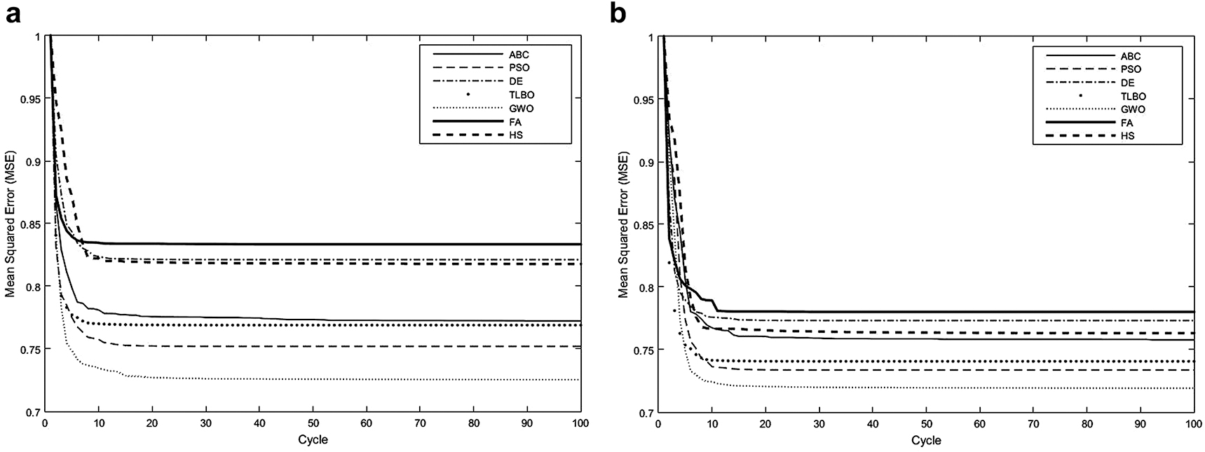
Figure 7 represents the convergence speeds of the algorithms for the retinal images given in Figure 1 (b) and Figure 2 (a). For a fair and detailed comparison, the convergence speeds have been given for both an abnormal retinal image from DRIVE database and a normal retinal image from STARE database. The evolution of best solutions has been obtained based on MSE. As seen from Figure 7 (a) which shows the convergence speeds obtained for the normal retinal image taken from DRIVE database, each algorithm needs approximately 10 cycles to converge to the optimal solution and the MSE performance of the GWO algorithm seems a bit better than the other algorithms. On the other hand, Figure 7 (b) shows the convergence speeds of the algorithms for the abnormal retinal image taken from STARE database. It is seen that each algorithm reaches to the global solution at 15 cycles. Also, the MSE performance of GWO seems a bit better than the other algorithms. According to the simulation results it is clear that convergence speeds and MSE performances of the algorithms in terms of clustering is close to each other.

Figure 7:

Convergence speed of the algorithms.

(a) Convergence speeds of the algorithms for the retinal image taken from DRIVE database given in Figure 1b. (b) Convergence speeds of the algorithms for the retinal image taken from STARE database given in Figure 2a.

Another important performance criterion for heuristic algorithms is the standard deviation which determines the stability of the algorithm. The low standard deviation indicates that the algorithm approximates similar error values at each random run. Table 10 and Table 11 contain the standard deviations obtained after 20 random runs for the retinal images taken from DRIVE and STARE databases. In addition to the standard deviation, the minimum MSE values reached by the algorithms have been shown in the tables. When the minimum MSE values reached by the algorithms are examined it is seen that all the algorithms produce similar MSE values, in other words, their clustering performance are very close to each other. On the other hand, due to their lower standard deviation values for the image taken from DRIVE database PSO and HS algorithms seem a little more stable in terms of clustering when compared to other algorithms. Similarly PSO, TLBO and HS algorithms are said to be a little more stable than the other algorithms for the image taken from STARE database.

References

1. Fong, DS, Aiello, L, Gardner, TW. Retinopathy in diabetes. Diabetes Care 2004;27:84–7. https://doi.org/10.2337/diacare.27.2007.s84.Search in Google Scholar
2. Fraz, MM, Remagnino, P, Hoppe, A, Uyyanonvara, B, Rudnicka, AR, Owen, CG, et al.. Blood vessel segmentation methodologies in retinal images-a survey. Comput Methods Progr Biomed 2012;108:407–33. https://doi.org/10.1016/j.cmpb.2012.03.009.Search in Google Scholar
3. Wang, JJ, Taylor, B, Wong, TY, Chua, B, Rochtchina, E, Klein, R, et al.. Retinal vessel diameters and obesity: a population-based study in older persons. Obesity 2006;14:206–14. https://doi.org/10.1038/oby.2006.27.Search in Google Scholar
4. Foracchia, M, Grisan, E, Ruggeri, A. Extraction and quantitative description of vessel features in hypertensive retinopathy fundus images. In: 2th Int workshop on comput assisted fundus image anal (CAFIA-2). Copenhagen, Denmark; 2001:5–7 pp.Search in Google Scholar
5. Mitchell, P, Leung, H, Wang, JJ, Rochtchina, E, Lee, AJ, Wong, TY, et al.. Retinal vessel diameter and open-angle glaucoma: the blue mountains eye study. Ophthalmology 2005;112:245–50. https://doi.org/10.1016/j.ophtha.2004.08.015.Search in Google Scholar
6. Goatman, K, Charnley, A, Webster, L, Nussey, S. Assessment of automated disease detection in diabetic retinopathy screening using two-field photography. PloS One 2011;6:275–84. https://doi.org/10.1371/journal.pone.0027524.Search in Google Scholar
7. Asad, AH, Elamry, E, Hassanien, AE, Tolba, MF. New global update mechanism of ant colony system for retinal vessel segmentation. In: 13th IEEE Int conf hybrid intell syst (HIS13) Tunisia; 2013:222–8 pp.10.1109/HIS.2013.6920486Search in Google Scholar
8. Verma, K, Deep, P, Ramakrishnan, AG. Detection and classification of diabetic retinopathy using retinal images flight. In: IEEE annu India conf (INDICON). Hyderabad, India; 2011:1–6 pp.10.1109/INDCON.2011.6139346Search in Google Scholar
9. Heneghan, C, Flynn, J, OKeefe, M, Cahill, M. Characterization of changes in blood vessel width and tortuosity in retinopathy of prematurity using image analysis. Med Image Anal 2002;6:407–29. https://doi.org/10.1016/s1361-8415(02)00058-0.Search in Google Scholar
10. Lowell, J, Hunter, A, Steel, D, Basu, A, Ryder, R, Kennedy, RL. Measurement of retinal vessel widths from fundus images based on 2D modeling. IEEE Trans Med Imag 2004;23:1196–204. https://doi.org/10.1109/tmi.2004.830524.Search in Google Scholar
11. Haddouche, A, Adel, M, Rasigni, M, Conrath, J, Bourennane, S. Detection of the foveal avascular zone on retinal angiograms using Markov random fields. Digit Signal Process 2010;20:149–54. https://doi.org/10.1016/j.dsp.2009.06.005.Search in Google Scholar
12. Grisan, E, Ruggeri, A. A divide etimpera strategy for automatic classification of retinal vessels into arteries and veins. Engineering in medicine and biology society. In: 25th IEEE annu Int conf. Cancun, Mexico; 2003:890–93 pp.Search in Google Scholar
13. Kanski, JJ. Clinical ophthalmology, 6th ed. London: Elsevier Health Sciences; 2007.Search in Google Scholar
14. Archer, DB. Diabetic retinopathy: some cellular. molecular and therapeutic considerations. Eye 1999;13:497–523. https://doi.org/10.1038/eye.1999.130.Search in Google Scholar
15. Antal, B, Hajdu, A. An ensemble-based system for microaneurysm detection and diabetic retinopathy grading. IEEE Trans Biomed Eng 2012;59:1720–6. https://doi.org/10.1109/tbme.2012.2193126.Search in Google Scholar
16. Abramoff, MD, Folk, JC, Han, DP. Automated analysis of retinal images for detection of referable diabetic retinopathy. JAMA Ophthalmol 2013;131:351–7. https://doi.org/10.1001/jamaophthalmol.2013.1743.Search in Google Scholar
17. Foracchia, M, Grisan, E, Ruggeri, A. Detection of optic disc in retinal images by means of a geometrical model of vessel structure. IEEE Trans Med Imag 2004;23:1189–95. https://doi.org/10.1109/tmi.2004.829331.Search in Google Scholar
18. Engelbrecht, AP. Fundamentals of computational swarm intelligence. Chichester, UK: John Wiley & Sons Publication; 2005.Search in Google Scholar
19. Karaboga, D. An idea based on honey bee swarm for numerical optimization. Technical Report-TR06. Kayseri, Turkey: Erciyes University, Engineering Faculty, Computer Engineering Department; 2005.Search in Google Scholar
20. Eberhart, RC, Kennedy, J. A new optimizer using particle swarm theory. In: 6th IEEE Int symp micromachine hum sci. Nagoya, Japan; 1995:39–43 pp.10.1109/MHS.1995.494215Search in Google Scholar
21. Storn, R, Price, K. Differential evolution- a simple and efficient adaptive scheme for global optimization over continuous spaces. Technical Report TR-95-012. Berkeley, California USA; 1995.Search in Google Scholar
22. Rao, RV, Patel, V. An elitist teaching-learning-based optimization algorithm for solving complex constrained optimization problems. Int J Ind Syst Eng Comput 2012;3:535–60. https://doi.org/10.5267/j.ijiec.2012.03.007.Search in Google Scholar
23. Mirjalili, SM, Lewis, A. Grey wolf optimizer. Adv Eng Software 2014;69:46–61. https://doi.org/10.1016/j.advengsoft.2013.12.007.Search in Google Scholar
24. Song, X, Tang, L, Zhao, S, Zhang, X, Li, L, Huang, J, et al.. Grey wolf optimizer for parameter estimation in surface waves. Soil Dynam Earthq Eng 2015;75:147–57. https://doi.org/10.1016/j.soildyn.2015.04.004.Search in Google Scholar
25. Mirjalili, S. How effective is the grey wolf optimizer in training multi-layer perceptrons. Appl Intell 2015;43:150–61. https://doi.org/10.1007/s10489-014-0645-7.Search in Google Scholar
26. Yang, XS. Firefly algorithms for multimodal optimization in stochastic algorithms: foundations and applications. Lect Notes Eng Comput Sci 2009;5792:169–78. https://doi.org/10.1007/978-3-642-04944-6_14.Search in Google Scholar
27. Lee, KS, Geem, ZW. A new meta-heuristic algorithm for continuous engineering optimization: harmony search theory and practice. Comput Methods Appl Mech Eng 2005;194:3902–33. https://doi.org/10.1016/j.cma.2004.09.007.Search in Google Scholar
28. Mahdavi, M, Fesanghary, M, Damangir, E. An improved harmony search algorithm for solving optimization problems. Appl Math Comput 2007;188:1567–79. https://doi.org/10.1016/j.amc.2006.11.033.Search in Google Scholar
29. Hoover, A, Kouznetsova, V, Goldbaum, M. Locating blood vessels in retinal images by piece wise threshold probing of a matched filter response. IEEE Trans Med Imag 2000;19:203–10. https://doi.org/10.1109/42.845178.Search in Google Scholar
30. Alonso-Montes, C, Vilariño, DL, Dudek, P, Penedo, MG. Fast retinal vessel tree extraction: a pixel parallel approach. Int J Circ Theor Appl 2008;36:641–51. https://doi.org/10.1002/cta.512.Search in Google Scholar
31. You, X, Peng, Q, Yaun, Y, Cheng, Y, Lei, J. Segmentation of retinal blood vessels using the radial projection and semi-supervised approach. Pattern Recogn 2011;44:2314–24. https://doi.org/10.1016/j.patcog.2011.01.007.Search in Google Scholar
32. Roychowdhury, S, Koozekanani, DD, Parhi, KK. Blood vessel segmentation of fundus images by major vessel extraction and subimage classification. IEEE J Biomed Health Inf 2015;19:1118–28.10.1109/JBHI.2014.2335617Search in Google Scholar
33. Wang, S, Yin, Y, Cao, G, Wei, B, Zheng, Y, Yang, G. Hierarchical retinal blood vessel segmentation based on feature and ensemble learning. Neurocomputing 2015;149:708–17. https://doi.org/10.1016/j.neucom.2014.07.059.Search in Google Scholar
34. Mendonca, AM, Campilho, A. Segmentation of retinal blood vessels by combining the detection of centerlines and morphological reconstruction. IEEE Trans Med Imag 2006;25:1200–13. https://doi.org/10.1109/tmi.2006.879955.Search in Google Scholar
35. Azzopardi, G, Strisciuglio, N, Vento, M, Petkov, N. Trainable COSFIRE filters for vessel delineation with application to retinal images. Med Image Anal 2015;19:46–57. https://doi.org/10.1016/j.media.2014.08.002.Search in Google Scholar
36. Fraz, MM, Remagnino, P, Hoppe, A, Uyyanonvara, B, Rudnicka, AR, Owen, CG, et al.. An ensemble classification-based approach applied to retinal blood vessel segmentation. IEEE Trans Biomed Eng 2012;59:2538–48. https://doi.org/10.1109/tbme.2012.2205687.Search in Google Scholar
37. Odstrcilik, J, Kolar, R, Budai, A, Hornegger, J, Jan, J, Gazarek, J, et al.. Retinal vessel segmentation by improved matched filtering: evaluation on a new high-resolution fundus image database. IET Image Process 2013;7:373–83. https://doi.org/10.1049/iet-ipr.2012.0455.Search in Google Scholar
38. Marín, D, Aquino, A, Gegúndez-Arias, ME, Bravo, JM. A new supervised method for blood vessel segmentation in retinal images by using gray-level and moment invariants-based features. IEEE Trans Med Imag 2011;30:146–58. https://doi.org/10.1109/tmi.2010.2064333.Search in Google Scholar
39. Kaba, D, Wang, C, Li, Y, Salazar-Gonzalez, A, Liu, X, Serag, A. Retinal blood vessels extraction using probabilistic modelling. Health Inf Sci Syst 2014;27:2.10.1186/2047-2501-2-2Search in Google Scholar PubMed PubMed Central
40. Dash, J, Bhoi, N. A thresholding based technique to extract retinal blood vessels from fundus images. Future Comp Inf J 2017;2:103–9. https://doi.org/10.1016/j.fcij.2017.10.001.Search in Google Scholar
41. Argüello, F, Vilariño, DL. Heras, DB. Nieto, A. GPU-based segmentation of retinal blood vessels. J Real-Time Image Process 2014;14:1–10. https://doi.org/10.1007/s11554-014-0469-z.Search in Google Scholar
42. Asad, AH, Azar, AT, Hassanien, AE. Ant colony-based system for retinal blood vessels segmentation. In: 7th Int conf bio-inspired comput theor and appl (BIC-TA 2012). Gwalior, India; 2012:441–52 pp.10.1007/978-81-322-1038-2_37Search in Google Scholar
43. Zhao, YQ, Wang, XH, Wang, XF, Shih, FY. Retinal vessels segmentation based on level set and region growing. Pattern Recogn 2014;47:2437–46.10.1016/j.patcog.2014.01.006Search in Google Scholar
44. Zhang, B, Zhang, L, Karray, F. Retinal vessel extraction by matched filter with first-order derivative of Gaussian. Comput Biol Med 2010;40:438–45. https://doi.org/10.1016/j.compbiomed.2010.02.008.Search in Google Scholar
45. Imani, E, Javidi, M, Pourreza, HR. Improvement of retinal blood vessel detection using morphological component analysis. Comput Methods Progr Biomed 2015;118:263–79. https://doi.org/10.1016/j.cmpb.2015.01.004.Search in Google Scholar
46. Mendonca, A, Dashtbozorg, B, Campilho, A. Segmentation of the vascular network of the retina. Image Anal Model Ophthalmol 2014:85–109. https://doi.org/10.1201/b16510-6.Search in Google Scholar
47. Xiao, Z, Adel, M, Bourennane, S. Bayesian method with spatial constraint for retinal vessel segmentation. Comput Math Methods Med 2013. https://doi.org/10.1109/icassp.2013.6637899.Search in Google Scholar
48. Fraz, MM, Remagnino, P, Hoppe, A, Uyyanonvara, B, Rudnicka, AR, Owen, CG, et al.. An ensemble classification-based approach applied to retinal blood vessel segmentation. IEEE Trans Biomed Eng 2012;59:2538–48. https://doi.org/10.1109/tbme.2012.2205687.Search in Google Scholar
49. Yin, B, Li, H, Sheng, B, Hou, X, Chen, Y, Wu, W, et al.. Vessel extraction from non-fluorescein fundus images using orientation-aware detector. Med Image Anal 2015;26:232–42. https://doi.org/10.1016/j.media.2015.09.002.Search in Google Scholar
50. Lázár, I, Hajdu, A. Segmentation of retinal vessels by means of directional response vector similarity and region growing. Comput Biol Med 2015;66:209–21. https://doi.org/10.1016/j.compbiomed.2015.09.008.Search in Google Scholar
51. Strisciuglio, N, Azzopardi, G, Vento, M, Petkov, N. Multiscale blood vessel delineation using b-cosfire filters. In: Springer Int conf comput anal images and patterns. Valletta, Malta; 2015:300–12 pp.10.1007/978-3-319-23117-4_26Search in Google Scholar
© 2020 Mehmet Bahadır Çetinkaya and Hakan Duran, published by De Gruyter, Berlin/Boston
This work is licensed under the Creative Commons Attribution 4.0 International License.
Articles in the same Issue
- Frontmatter
- Research Articles
- Nonlinear analysis of scalp EEGs from normal and brain tumour subjects
- Dimensionality reduction for EEG-based sleep stage detection: comparison of autoencoders, principal component analysis and factor analysis
- EEG signal classification based on SVM with improved squirrel search algorithm
- The effect of attentional focusing strategies on EMG-based classification
- Identification of dental pain sensation based on cardiorespiratory signals
- ScatT-LOOP: scattering tetrolet-LOOP descriptor and optimized NN for iris recognition at-a-distance