Network Investments Under Different Consumer Expectations and Competition Modes

A.1 Comparative Statics

We can rewrite the FOCs given in eq. (6) and eq. (7), such that F l k s l k , n ̄ , σ = 0 , k ∈ {C, B} (where C(B) stands for the Cournot (Bertrand) case), and l ∈ {p, r} (where p(r) stands for passive (responsive) expectations). Total differentiation of the FOCs can then be expressed as

which can be used to show that

Note that the SOC requires ∂ F l k [ ⋅ ] / ∂ s l k < 0 , which leads to

A.2 Proof of Proposition 2

Following the expression in eq. (A.1), and using eq. (A.3) and eq. (A.4) (for the case of Cournot under passive expectations), and eq. (A.7) and eq. (A.8) (for the case of Bertrand under passive expectations), the slope of each level-curve can be expressed as:

Appendix A.1 has already proved that d n ̄ / d σ | d s p C = 0 > 0 iff n < (1 + 2σ)/2(1 + σ) and d n ̄ / d σ | d s p B = 0 > 0 iff n < (1 − (2 − 3σ)σ)/2, where (1 + 2σ)/2(1 + σ) > (1 − σ(2 − 3σ))/2. It is straightforward to show that:

As for the loci of the iso-investment (level) curves, denoted s p k [ n ̄ , σ ] , k ∈ {C, B}, the FOCs given in eq. (6) are used. Evaluating the FOCs at a common investment level, s p B = s p C = s ̃ , for which F p k s p k = s ̃ , n ̄ , σ = 0 , k ∈ {C, B}, for any n ̄ ∈ ( 0,1 ) , and σ ∈ (0, 1), proves that

1. Lim σ → 0 F p C s p C = s ̃ , n ̄ , σ ≃ Lim σ → 0 F p B s p B = s ̃ , n ̄ , σ = 0 (that is, as σ tends to zero, the two level-curves tend to each other on the same graph, where n ̄ (σ) is on the vertical (horizontal) axis (see the magenta and red curves in Figure A.1);

2. F p C s p C = s ̃ , n ̄ , σ ≃ F p B s p B = s ̃ , n ̄ , σ = 0 at n = 1 − Δ / ( 2 3 ( 1 + σ ) 2 ) − ( 2 3 1 − σ 2 ) / Δ , where

3.      Δ = 2 + ( 1 − σ ) 2 b 4 ( 1 + σ ) 8 + σ 6 + σ σ σ 4 + 3 σ 3 − 8 σ − 7 + 3 3 ; and n ∈ (0, 1) if σ > 0.6, or negative if otherwise (that is, the two level-curves at the same investment level satisfying the FOCs intersect at a threshold network strength, which is increasing in σ (see the black-dashed curve in Figure A.1).

Figure A.1:

Cournot versus Bertrand under passive expectations.

Note that ( 3 σ ( 1 + σ ) − 2 ) / 2 ( 1 + σ ) > ( 1 − Δ / ( 2 3 ( 1 + σ ) 2 ) − ( 2 3 1 − σ 2 ) / Δ ) . Clearly, from eq. (A.13), s p B [ n ̄ , σ ] ≡ s ̃ is above s p C [ n ̄ , σ ] ≡ s ̃ for n < 1 − Δ / ( 2 3 ( 1 + σ ) 2 ) − ( 2 3 1 − σ 2 ) / Δ , and below s p B [ n ̄ , σ ] ≡ s ̃ otherwise.

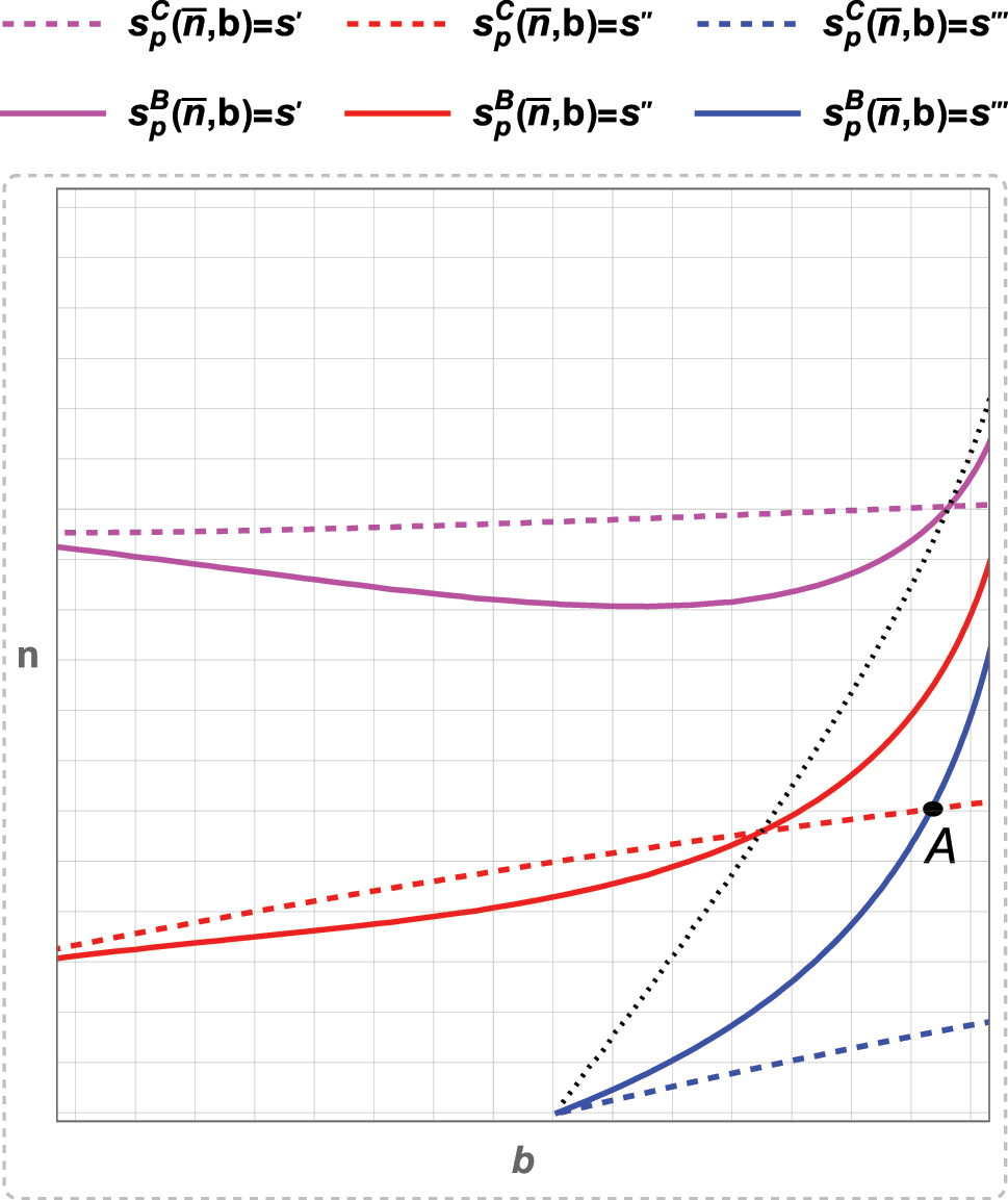
Iso-investment (level) curves for three different investment levels along with the threshold network strength are plotted in Figure A.1. The colored-dashed curves represent the case of Cournot competition under passive consumer expectations, whereas the colored-solid curves represent the case of Bertrand competition under passive expectations. In both cases, a higher investment level requires a shift in the level-curve above and to the left, that is, the magenta-colored curves are plotted at a higher investment level, s′, that satisfies the FOCs in eq. (6) than the red-colored curves (along which the investment level is s″), while the blue-colored curves are plotted for the lowest investment level, s‴, for which the two level-curves at the same investment level satisfying their respective FOCs still intersect. The black-dashed curve represents all the (σ, n) pairs at which the two level-curves at the same investment level satisfy their respective FOCs, that is, the plot of n = 1 − Δ / ( 2 3 ( 1 + σ ) 2 ) − ( 2 3 1 − σ 2 ) / Δ . As is already proved above, to the left and above the black-dashed curve, s p C [ n ̄ , σ ] ≡ s ̃ is above s p B [ n ̄ , σ ] ≡ s ̃ , that is, for a given σ and n ̄ , for which s ̃ is the optimal investment level for a Cournot firm facing passive consumer expectations, a higher investment level s > s ̃ will be optimal for a Bertrand firm facing passive consumer expectations. By the same token, to the right and below the black-dashed curve, s p C [ n ̄ , σ ] ≡ s ̃ is below s p B [ n ̄ , σ ] ≡ s ̃ , that is, for a given σ and n ̄ , for which s ̃ is the optimal investment level for a Bertrand firm facing passive consumer expectations, a higher investment level s > s ̃ will be optimal for a Cournot firm facing passive consumer expectations. This is also illustrated in Figure A.1 at point A, where s‴ is the optimal investment level for a Bertrand firm, whereas a higher investment level, s″, is optimal for a Cournot firm.

This completes the proof of Proposition 2 suggesting that the equilibrium level of investments strengthening network effects under passive consumer expectations is higher for Bertrand firms than for Cournot firms for σ ≤ 0.6 (for which s p C [ n ̄ , σ ] ≡ s ̃ is always above s p B [ n ̄ , σ ] ≡ s ̃ ). As for σ > 0.6, there exists a minimum network strength threshold (which is increasing in σ), above (below) which, the optimal investment level is higher (lower) for Bertrand firms than for Cournot firms.

A.3 Proof of Proposition 4

A.3.1 Passive versus Responsive Expectations: Cournot Competition

Following the expression in eq. (A.1), and using eq. (A.5) and eq. (A.6), the slope of the level-curves in the case of Cournot competition under responsive expectations can be expressed as:

(A.14) d n ̄ d σ d s r C = 0 = ( 1 − n ) ( 2 + σ ) > 0 .

Comparing the expressions in eq. (A.14) and in eq. (A.11) suggests that:

(A.15) d n ̄ d σ d s p C = 0 < 0 < d n ̄ d σ d s r C = 0   if   n > ( 1 + 2 σ ) 2 ( 1 + σ ) ; 0 < d n ̄ d σ d s p C = 0 < d n ̄ d σ d s r C = 0   if   n < ( 1 + 2 σ ) 2 ( 1 + σ ) .

As for the loci of the iso-investment (level) curves, denoted s l C [ n ̄ , σ ] , l ∈ {p, r}, the FOCs for the case of passive expectations given in eq. (6) and for the case of responsive expectations given in eq. (7) are used. Evaluating the FOCs at a common investment level, s p C = s r C = s ̃ , for which F l C s l C = s ̃ , n ̄ , σ = 0 , l ∈ {p, r}, for any n ̄ ∈ ( 0,1 ) , and σ ∈ (0, 1), proves that

1. Lim σ → 0 F p C s p C = s ̃ , n ̄ ̃ , σ ≃ Lim σ → 0 F r C s r C = s ̃ , n ̄ , σ = 0 , where n ̄ ̃ > n ̄ (that is, as σ tends to zero, for the same investment level, the FOC for the case of responsive expectations is fulfilled at lower network strength, suggesting the level-curve s p C [ n ̄ , σ ] ≡ s ̃ is above s r C [ n ̄ , σ ] ≡ s ̃ as σ tends to zero (see the magenta and red curves in Figure A.2);

2. Lim σ → 1 F p C s p C = s ̃ , n ̄ ̃ , σ ≃ Lim σ → 1 F r C s r C = s ̃ , n ̄ , σ = 0 , where n ̄ ̃ < n ̄ for n ∈ (0, 0.59), or n ̄ ̃ > n ̄ otherwise (that is, as σ tends to one, for the same investment level, the FOC for the case of responsive expectations is fulfilled at higher network strength so long as the network strength is below a threshold, suggesting the level-curve s p C [ n ̄ , σ ] ≡ s ̃ is below (above) s r C [ n ̄ , σ ] ≡ s ̃ if the network strength is below (above) the threshold value as σ tends to one (see the magenta, red and blue curves in Figure A.2);

3. F p C s p C = s ̃ , n ̄ , σ ≃ F r C s r C = s ̃ , n ̄ , σ = 0 at n ≡ g _C [σ], where Lim _σ→0 g _C [σ] = 0 and Lim _σ→1 g _C [σ] = 0.59 (that is, the two level-curves at the same investment level satisfying the FOCs intersect at a threshold network strength that extends between the (σ, n)-coordinates (0,0) and (1,0.59) (see the black-dashed curve plotted in Figure A.2 for all (σ, n) that fulfills F p C s p C = s ̃ , n ̄ , σ ≃ F r C s r C = s ̃ , n ̄ , σ = 0 ).

Figure A.2:

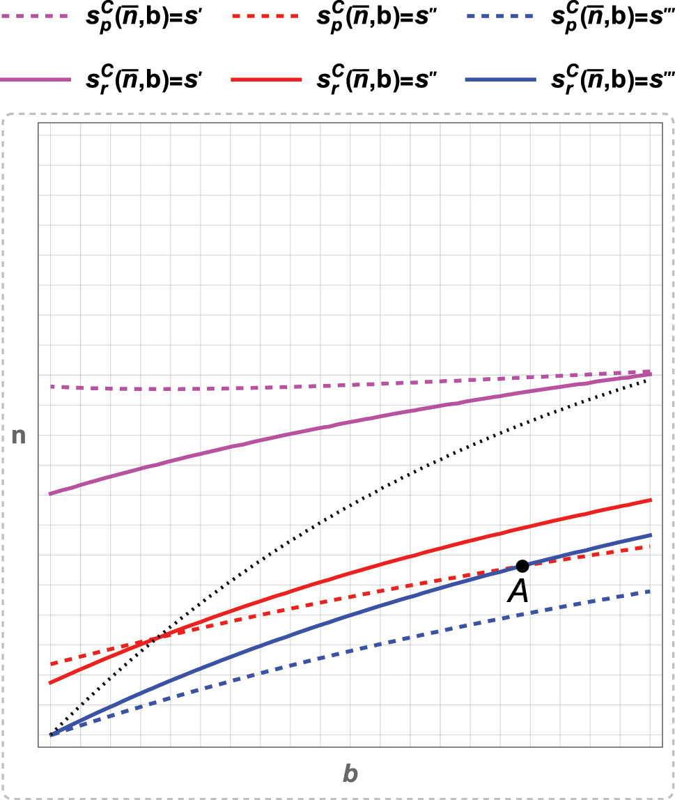
Passive versus responsive expectations: Cournot.

Iso-investment (level) curves for three different investment levels along with the threshold network strength are plotted in Figure A.2. The colored-dashed curves represent the case of passive consumer expectations, whereas the colored-solid curves represent the case of responsive expectations for Cournot firms. In both cases, a higher investment level requires a shift in the level-curve above and to the left, that is, the magenta-colored curves are plotted for the highest investment level, s′, for which the two level-curves at the same investment level satisfying their respective FOCs given in eq. (6) and in eq. (7) still intersect. Along the red-colored curves the investment level, s″), is lower, while the blue-colored curves are plotted for the lowest investment level, s‴, for which the two level-curves at the same investment level satisfying their respective FOCs still intersect. The black-dashed curve represents all the (σ, n) pairs at which the two level-curves at the same investment level satisfy their respective FOCs, that is, the plot of n = g _C [σ] that fulfills F p C s p C = s ̃ , n ̄ , σ ≃ F r C s r C = s ̃ , n ̄ , σ = 0 . As is already proved above, to the left and above the black-dashed curve, s p C [ n ̄ , σ ] ≡ s ̃ is above s r C [ n ̄ , σ ] ≡ s ̃ , that is, for a given σ and n ̄ , for which s ̃ is the optimal investment level for a Cournot firm facing passive consumer expectations, a higher investment level s > s ̃ will be optimal for a Cournot firm facing responsive consumer expectations. By the same token, to the right and below the black-dashed curve, s p C [ n ̄ , σ ] ≡ s ̃ is below s r C [ n ̄ , σ ] ≡ s ̃ , that is, for a given σ and n ̄ , for which s ̃ is the optimal investment level for a Cournot firm facing responsive consumer expectations, a higher investment level s > s ̃ will be optimal for a Cournot firm facing passive consumer expectations. This is also illustrated in Figure A.2 at point A, where s‴ is the optimal investment level for a Cournot firm facing responsive expectations, whereas a higher investment level, s″, is optimal for a Cournot firm facing passive expectations.

A.3.2 Passive versus Responsive Expectations: Bertrand Competition

Following the expression in eq. (A.1), and using eq. (A.9) and eq. (A.10), the slope of the level-curves in the case of Bertrand competition under responsive expectations can be expressed as:

(A.16) d n ̄ d σ d s r B = 0 = ( 1 − ( 1 − σ ) σ ) ( 1 − n ) ( 2 − σ ) ( 1 − σ 2 ) > 0 .

Comparing the expressions in eq. (A.16) and in eq. (A.12) suggests that:

(A.17) d n ̄ d σ d s p B = 0 < 0 < d n ̄ d σ d s r B = 0   if   n > ( 1 − σ ( 2 − 3 σ ) ) 2 ; 0 < d n ̄ d σ d s p B = 0 < d n ̄ d σ d s r B = 0   if   n < ( 1 − σ ( 2 − 3 σ ) ) 2 .

As for the loci of the iso-investment (level) curves, denoted s l B [ n ̄ , σ ] , l ∈ {p, r}, the FOCs for the case of passive expectations given in eq. (6) and for the case of responsive expectations given in eq. (7) are used. Evaluating the FOCs at a common investment level, s p B = s r B = s ̃ , for which F l B s l B = s ̃ , n ̄ , σ = 0 , l ∈ {p, r}, for any n ̄ ∈ ( 0,1 ) , and σ ∈ (0, 1), proves that

1. Lim σ → 0 F p B s p B = s ̃ , n ̄ ̃ , σ ≃ Lim σ → 0 F r B s r B = s ̃ , n ̄ , σ = 0 , where n ̄ ̃ > n ̄ (that is, as σ tends to zero, for the same investment level, the FOC for the case of responsive expectations is fulfilled at lower network strength, suggesting the level-curve s p B [ n ̄ , σ ] ≡ s ̃ is above s r B [ n ̄ , σ ] ≡ s ̃ as σ tends to zero (see the magenta and red curves in Figure A.3);

2. Lim σ → 1 F p B s p B = s ̃ , n ̄ ̃ , σ ≃ Lim σ → 1 F r B s r B = s ̃ , n ̄ , σ = 0 , where n ̄ ̃ < n ̄ (that is, as σ tends to one, for the same investment level, the FOC for the case of responsive expectations is fulfilled at higher network strength, suggesting the level-curve s p B [ n ̄ , σ ] ≡ s ̃ is below s r B [ n ̄ , σ ] ≡ s ̃ as σ tends to one (see the magenta, red and blue curves in Figure A.3);

3. F p B s p B = s ̃ , n ̄ , σ ≃ F r B s r B = s ̃ , n ̄ , σ = 0 at n ≡ g _B [σ], where Lim _σ→0 g _B [σ] = 0 and Lim _σ→1 g _B [σ] = 1 (that is, the two level-curves at the same investment level satisfying the FOCs intersect at a threshold network strength that extends at the limit between the (σ, n)-coordinates (0,0) and (1,1) (see the black-dashed curve plotted in Figure A.3 for all (σ, n) that fulfills F p B s p B = s ̃ , n ̄ , σ ≃ F r B s r B = s ̃ , n ̄ , σ = 0 ).

Figure A.3:

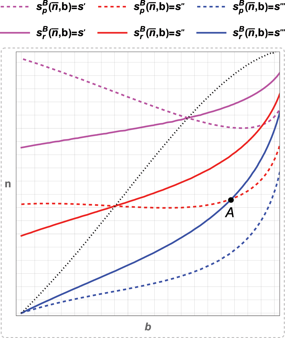
Passive versus responsive expectations: Bertrand.

Iso-investment (level) curves for three different investment levels along with the threshold network strength are plotted in Figure A.3. The colored-dashed curves represent the case of passive consumer expectations, whereas the colored-solid curves represent the case of responsive expectations for Bertrand firms. In both cases, a higher investment level requires a shift in the level-curve above and to the left, that is, the magenta-colored curves are plotted at a higher investment level, s′, that satisfies the FOCs in eq. (6) and in eq. (7), than the red-colored curves (along which the investment level is s″), while the blue-colored curves are plotted for the lowest investment level, s‴, for which the two level-curves at the same investment level satisfying their respective FOCs still intersect. The black-dashed curve represents all the (σ, n) pairs at which the two level-curves at the same investment level satisfy their respective FOCs, that is, the plot of n = g _B [σ] that fulfills F p B s p B = s ̃ , n ̄ , σ ≃ F r B s r B = s ̃ , n ̄ , σ = 0 . As is already proved above, to the left and above the black-dashed curve, s p B [ n ̄ , σ ] ≡ s ̃ is above s r B [ n ̄ , σ ] ≡ s ̃ , that is, for a given σ and n ̄ , for which s ̃ is the optimal investment level for a Bertrand firm facing passive consumer expectations, a higher investment level s > s ̃ will be optimal for a Bertrand firm facing responsive consumer expectations. By the same token, to the right and below the black-dashed curve, s p B [ n ̄ , σ ] ≡ s ̃ is below s r B [ n ̄ , σ ] ≡ s ̃ , that is, for a given σ and n ̄ , for which s ̃ is the optimal investment level for a Bertrand firm facing responsive consumer expectations, a higher investment level s > s ̃ will be optimal for a Bertrand firm facing passive consumer expectations. This is also illustrated in Figure A.3 at point A, where s‴ is the optimal investment level for a Bertrand firm facing responsive expectations, whereas a higher investment level, s″, is optimal for a Bertrand firm facing passive expectations.

A.4 Robustness of the Results: The Case of σ ≠ α

In the main text, we have presented the results for the case of α = σ. We now look at to what extent our results extend to the general case of α ≠ σ. Using the demand systems given in eqs.(2) and (3), maximizing profits leads to the following equilibrium output levels of each firm i ∈ {1, 2}:

under passive consumer expectations; or

under responsive consumer expectations, where superscript C and B represent Cournot and Bertrand, respectively. It is clear from eqs. (A.18) and (A.19) that positive outputs, which we assume throughout the paper, require n < min{1, (2 + σ)/(2 + α), (2 − σ)/(2 − α), (1 + σ)/(1 + α)}. As in Section 3, substituting the equilibrium outputs into the firms’ profit functions and differentiating them with respect to the investment levels, we can write the FOCs for Cournot and Bertrand firms in the first stage of the game, respectively, as in eq. (A.20), under passive consumer expectations:

or as in eq. (A.21), under responsive consumer expectations:

where Λ = (1 − n)[2(2 − α)(1 − σ − n(1 − α))(1 + σ − n(1 + α)) + (1 + α)(1 − σ − n(1 − α))(2 − σ − n(2 − α))] − [((1 − σ − n(1 − α)) + (1 − α)(1 − n))(2 − σ − n(2 − α))(1 + σ − n(1 + α))], and n = n ̄ + 2 s . We shall assume the SOCs are fulfilled. As in Section 3, we can differentiate the FOCs, given in Eqs.(A.20) and (A.21), with respect to the rival firm’s investment and show that investments are strategic complements in the Bulow et al. (1985) sense, so long as consumer expectations are passive. As for responsive consumer expectations, this would hold true only for a subset of permissible parameter values.

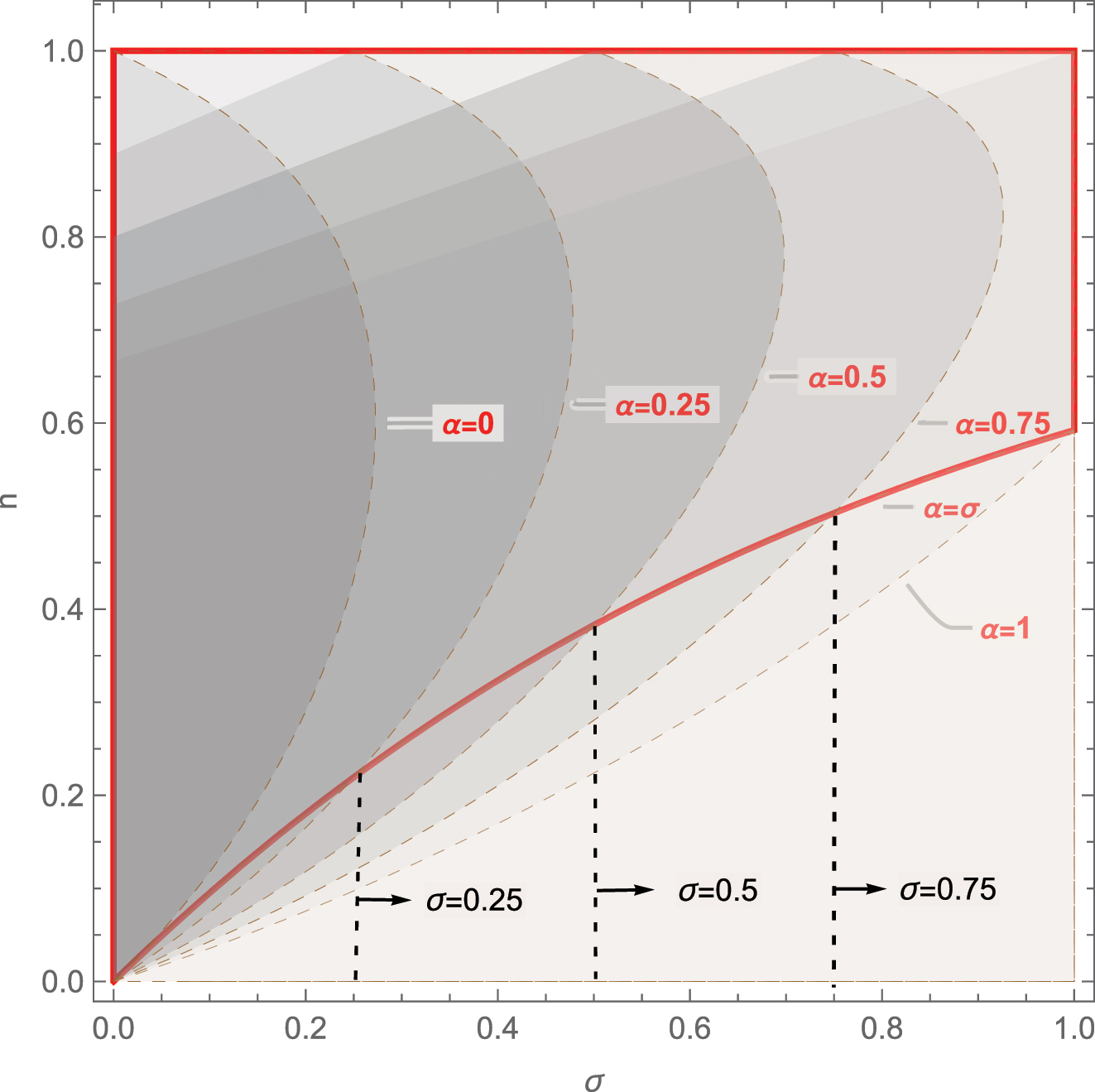
Using the two expressions given in eq. (A.20), we first compare the investment levels by Cournot versus Bertrand firms under passive consumer expectations, the results of which are given in Figure A.4.

Figure A.4:

Cournot versus Bertrand under passive expectations: α ≠ σ.

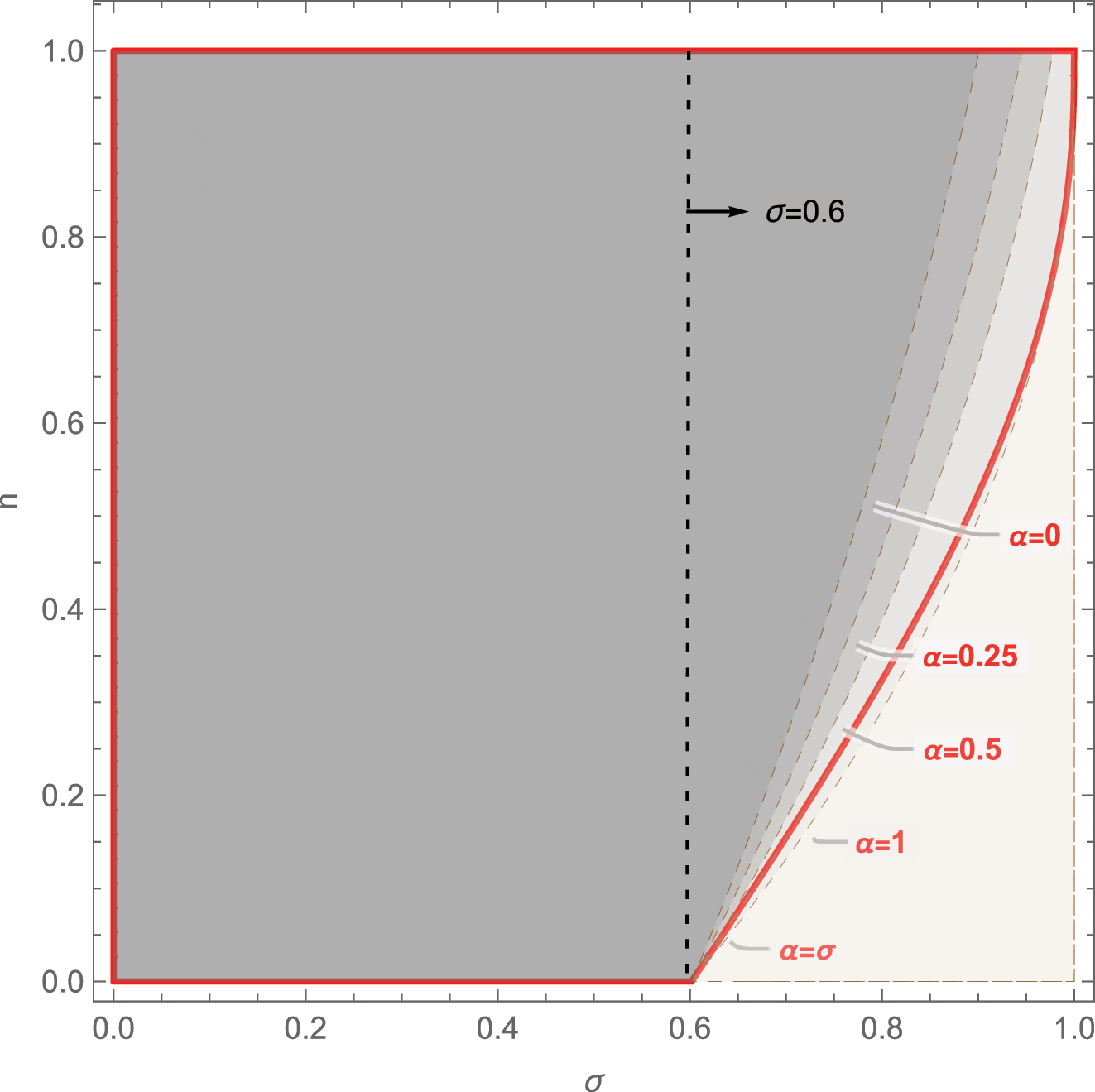
It is now clear from Figure A.4 that the result presented in Proposition 2 also extends to the case of α ≠ σ: Under passive consumer expectations, the equilibrium level of investments strengthening the network effects by Bertrand firms is higher for σ ≤ 0.6; as for σ > 0.6, there exists a minimum threshold network strength, above which (the shaded area above the dashed-brown curve) Bertrand firms invest more than Cournot firms under passive expectations; and below which (the shaded area below the dashed-brown curve) the opposite is true. Note that a lower value of α (lesser network compatibility) pushes up the boundary. The red-marked area corresponds to the one in which Bertrand firms invest more than Cournot firms under passive expectations when the extent of network compatibility is the same as that of product substitutability (α = σ). It appears that when the networks are fully compatible (when α = 1), it gets slightly more likely compared to the case of α = σ that Bertrand firms invest more than Cournot firms under passive expectations; notice the dashed-brown boundary at α = 1 is below the red-colored boundary, which is the same as the black-dashed curve in Figure A.1, given in Appendix A.2.

As for the investment incentives of Cournot versus Bertrand firms under responsive consumer expectations, comparing the two expressions given in eq. (A.21), we can now show that Proposition 3 also holds true, albeit for a subset of permissible parameter values. That is, under responsive expectations, the equilibrium investment level by Cournot firms is higher than that by Bertrand firms for α = 0 (perfect incompatibility) and for α ≤ σ, as is clear from Figure A.5. As for α ≥ σ, there exists a minimum threshold network strength, above which (the shaded areas above the dashed-brown lines) Bertrand firms invest more than Cournot firms.

Figure A.5:

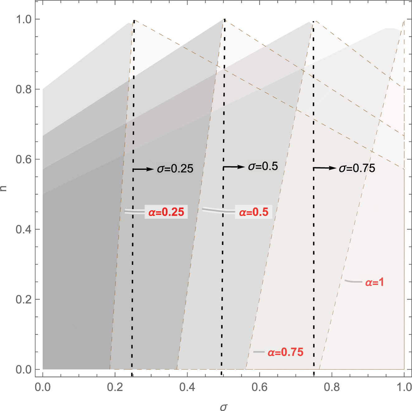
Cournot versus Bertrand under responsive expectations: α ≠ σ.

Note that, in Figure A.5, for each specific α-value (network compatibility), the permissible range of parameters are plotted as the shaded area plus the adjacent area marked with dashed-brown lines. In the shaded areas, investments by Bertrand firms are greater, whereas in the adjacent areas marked with dashed-brown lines, investments by Cournot firms are greater, under responsive expectations. The vertical dashed-black lines mark the specific values of σ, the degree of product substitutability. Clearly, for each specific α value (e.g., 0.25, 0.5, 0.75), the area to the right of the corresponding σ value, marked with the vertical dashed-black lines (i.e., α ≤ σ), falls into the area marked with dashed-brown lines, in which investments by Cournot firms are greater.

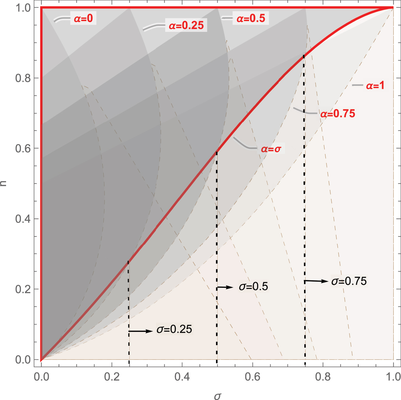
Next, we look at whether Proposition 4 survives in the general case. Using the expressions given in Eqs. (A.20) and (A.21), we compare the investment levels under passive versus responsive consumer expectations for a given competition mode (Cournot or Bertrand). Figure A.6 presents the results of the Cournot case, and Figure A.7 presents the results of the Bertrand case.

Figure A.6:

Passive versus responsive expectations: Cournot, α ≠ σ.

Figure A.7:

Passive versus responsive expectations: Bertrand, α ≠ σ.

It is now clear from both figures that the result presented in Proposition 4 also extends qualitatively to the case of α ≠ σ: The equilibrium investment levels are higher under responsive expectations than under passive expectations if the initial network strength is sufficiently high and the degree of product substitutability is sufficiently low. In both figures, the threshold network strength is marked by the dashed-brown curves, which expands to the right as network compatibility gets greater (as α increases). To the left of the dashed-brown threshold curves (in the shaded areas), responsive expectations result in higher investment. To the right of the dashed-brown threshold curves, the opposite holds true.

Note that for each specific α-value, the permissible range of parameters are plotted as the shaded area plus the complementary area to the right of the dashed-brown curves in Figure A.6, or plus the adjacent area marked with dashed-brown lines in Figure A.7. Moreover, in both figures, the vertical dashed-black lines mark the specific values of σ, the degree of product substitutability.

It should be noticed in both figures that, for each specific α-value, the intersection between the threshold dashed-brown curve and the vertical black-dashed line (the corresponding σ-value) is on the red-colored boundary, which is the same as the black-dashed curve in Figure A.2 in the Cournot case, and in Figure A.3 in the Bertrand case; see Appendix A.3. That is, in both Figures A.6 and A.7, the red-marked area corresponds to the one in which responsive expectations result in higher investment than passive expectations when the extent of network compatibility is the same as that of product substitutability (α = σ); see also Figure 1. It appears that when the networks are fully compatible (when α = 1), it gets slightly less likely compared to the case of α = σ that passive expectations result in higher investment than responsive expectations; notice the dashed-brown boundary at α = 1 is below the red-colored boundary in both figures.

References

Bhattacharjee, T., and R. Pal. 2014. “Network Externalities and Strategic Managerial Delegation in Cournot Duopoly: Is There a Prisoners’ Dilemma?” Review of Network Economics 12 (4): 343–53, https://doi.org/10.1515/rne-2013-0114.Search in Google Scholar
Boivin, C., and D. Vencatachellum. 2002. “R&D in Markets with Network Externalities.” Economics Bulletin 12 (9): 1–8.Search in Google Scholar
Buccella, D., L. Fanti, and L. Gori. 2023. “Strategic Product Compatibility in Network Industries.” Journal of Economics 140 (2): 141–68, https://doi.org/10.1007/s00712-023-00834-x.Search in Google Scholar
Bulow, J., J. Geanakoplos, and P. Klemperer. 1985. “Multimarket Oligopoly: Strategic Substitutes and Complements.” Journal of Political Economy 93 (3): 488–511, https://doi.org/10.1086/261312.Search in Google Scholar
Chirco, A., and M. Scrimitore. 2013. “Choosing Price or Quantity? the Role of Delegation and Network Externalities.” Economics Letters 121 (3): 482–6, https://doi.org/10.1016/j.econlet.2013.10.003.Search in Google Scholar
Economides, N. S. 1996. “Network Externalities, Complementarities, and Invitations to Enter.” European Journal of Political Economy 12 (2): 211–33. https://doi.org/10.1016/0176-2680-95-00014-3.Search in Google Scholar
Faulhaber, G. 2002. “Network Effects and Merger Analysis: Instant Messaging and the AOL-Time Warner Case.” Telecommunications Policy 26 (5-6): 311–33. https://doi.org/10.1016/s0308-5961-02-00015-0.Search in Google Scholar
Gandal, N. 2002. “Compatibility, Standardization and Network Effects: Some Policy Implications.” Oxford Review of Economic Policy 18 (1): 80–91, https://doi.org/10.1093/oxrep/18.1.80.Search in Google Scholar
Häckner, J. 2000. “A Note on Price and Quantity Competition in Differentiated Oligopolies.” Journal of Economic Theory 93 (2): 233–9, https://doi.org/10.1006/jeth.2000.2654.Search in Google Scholar
Hoernig, S. 2012. “Strategic Delegation Under Price Competition and Network Effects.” Economics Letters 117 (2): 487–9, https://doi.org/10.1016/j.econlet.2012.06.045.Search in Google Scholar
Hurkens, S., and A. López. 2014. “Mobile Termination, Network Externalities, and Consumer Expectations.” Economic Journal 124 (579): 1005–39.10.1111/ecoj.12097Search in Google Scholar
Katz, M. L., and C. Shapiro. 1985. “Network Externalities, Competition and Compatibility.” American Economic Review 75 (3): 424–40.Search in Google Scholar
Katz, M., and C. Shapiro. 1992. “Product Introduction with Network Externalities.” Journal of Industrial Economics 40 (1): 55–83. https://doi.org/10.2307/2950627.Search in Google Scholar
Koski, H., and T. Kretschmer. 2004. “Survey on Competing in Network Industries: Firm Strategies, Market Outcomes, and Policy Implications.” Journal of Industry, Competition and Trade 4 (1): 5–31, https://doi.org/10.1023/b-jict.0000029239.55756.e6.Search in Google Scholar
Kristiansen, E. G. 1996. “R&D in Markets with Network Externalities.” International Journal of Industrial Organisation 16 (6): 769–84.10.1016/0167-7187(96)01012-0Search in Google Scholar
Kristiansen, E. G. 1998. “R&D in the Presence of Network Externalities: Timing and Compatibility.” Rand Journal of Economics 29 (3): 531–47.10.2307/2556103Search in Google Scholar
Kristiansen, E. G., and M. Thum. 1997. “R&D Incentives in Compatible Networks.” Journal of Economics 65 (1): 55–78.10.1007/BF01239059Search in Google Scholar
Lee, D. J., K. Choi, and J. J. Han. 2018. “Strategic Delegation Under Fulfilled Expectations.” Economics Letters 169: 80–2, https://doi.org/10.1016/j.econlet.2018.05.016.Search in Google Scholar
Lee, D. J., K. Choi, and T. Nariu. 2020. “Endogenous Vertical Structure with Network Externalities.” Manchester School 88 (6): 827–46, https://doi.org/10.1111/manc.12342.Search in Google Scholar
Naskar, M., and R. Pal. 2020. “Network Externalities and Process R&D: A Cournot-Bertrand Comparison.” Mathematical Social Sciences 103: 51–8.10.1016/j.mathsocsci.2019.11.006Search in Google Scholar
Pal, R. 2014. “Price and Quantity Competition in Network Goods Duopoly: a Reversal Result.” Economics Bulletin 34 (3): 1019–27.Search in Google Scholar
Pal, R. 2015. “Cournot Vs. Bertrand Under Relative Performance Delegation: Implications of Positive and Negative Network Externalities.” Mathematical Social Sciences 75: 94–101, https://doi.org/10.1016/j.mathsocsci.2015.02.007.Search in Google Scholar
Saaskilahti, P. 2006. “Strategic R&D and Network Compatibility.” Economics of Innovation and New Technology 15 (8): 711–33.10.1080/10438590500510657Search in Google Scholar
Shrivastav, S. 2021. “Network Compatibility, Intensity of Competition and Process R&D: A Generalization.” Mathematical Social Sciences 109: 152–63.10.1016/j.mathsocsci.2020.12.003Search in Google Scholar
Singh, N., and X. Vives. 1984. “Price and Quantity Competition in a Differentiated Duopoly.” RAND Journal of Economics 15 (4): 546–54, https://doi.org/10.2307/2555525.Search in Google Scholar
Song, R., and L. F. S. Wang. 2017. “Collusion in a Differentiated Duopoly with Network Externalities.” Economics Letters 152: 23–6, https://doi.org/10.1016/j.econlet.2016.12.032.Search in Google Scholar
Sugiyama, T., B. Darling, and Y. Hayashi. 2025. ““Trade Distortion and Protectionism: Tariffs Hit Some Automakers More than Others” Report for the Hinrich Foundation.” https://www.hinrichfoundation.com/research/article/trade-distortion-and-protectionism/tariffs-hit-some-automakers-more-than-others/ (accessed July 22, 2025).Search in Google Scholar
Toshimitsu, T. 2016. “Price and Quantity Competition in a Differentiated Duopoly with Network Compatibility Effects.” Japanese Economic Review 67 (4): 495–512, https://doi.org/10.1111/jere.12109.Search in Google Scholar
Toshimitsu, T. 2019. “Comment on “Price and Quantity Competition in Network Goods Duopoly: a Reversal Result.” Economics Bulletin 39 (4): 1855–9.Search in Google Scholar
Xing, M. 2014. “On the Optimal Choices of R&D Risk in a Market with Network Externalities.” Economic Modelling 38 (February): 71–4.10.1016/j.econmod.2013.12.024Search in Google Scholar
© 2025 Walter de Gruyter GmbH, Berlin/Boston