
Game Theory Without Partitions, and Applications to Speculation and Consensus
-
John Geanakoplos


Abstract
Decision theory and game theory are extended to allow for information processing errors. This extended theory is then used to reexamine market speculation and consensus, both when all actions (opinions) are common knowledge and when they may not be. Five axioms of information processing are shown to be especially important to speculation and consensus. They are called nondelusion, knowing that you know (KTYK), nested, balanced, and positively balanced. We show that it is necessary and sufficient that each agent's information processing errors be (1) nondeluded and balanced so that the agents cannot agree to disagree, (2) nondeluded and positively balanced so that it cannot be common knowledge that they are speculating, and (3) nondeluded and KTYK and nested so that agents cannot speculate in equilibrium. Each condition is strictly weaker than the next one, and the last is strictly weaker than partition information.
“Is there any other point to which you would wish to draw my attention?”
“To the incident of the dog in the night-time.”
“The dog did nothing in the night-time.”
“That was the curious incident,” remarked Sherlock Holmes.
Sherlock Holmes is the perfectly rational Bayesian optimizer that economic models assume all agents are like. Yet most economic actors are probably much more like Dr. Watson, than like Sherlock Holmes. They usually take signals at face value. They often take no notice when something doesn't happen. They occasionally ignore unpleasant information. They forget. And sometimes their opinions will not budge unless confronted by proof.
The aim of this paper is to develop a coherent definition of equilibrium in games that allows for such errors in information processing. My point of view is that behavior may be only boundedly rational, but it need not be any the less goal oriented and purposeful, and therefore any the less predictable.
The bulk of this paper is devoted to analyzing the phenomenon of market speculation, and “agreements to disagree.” By now it is well known that neither of these commonplace events can be observed in equilibrium in a model of Bayesian rational agents. When agents are allowed to make errors in information processing, however, these phenomena do eventually emerge in equilibrium. The “curious incident” is the precise stage of irrationality at which they emerge. It is not true, for example, that an agent who always ignores unpleasant information is necessarily a sucker for a bet. It turns out that there is a substantial degree of information processing error (which is characterized here) that can occur, and still agents will not speculate against each other in equilibrium. There is a greater degree of irrationality, which can be specified exactly, that if not exceeded will keep agents from speculating against each other when those actions are common knowledge. And finally there is a still more serious kind of error, which again can be stated precisely, which if not exceeded will never permit agents to agree to disagree.
1 Errors in Information Processing
There are a number of errors that are typically made by decision makers that suggest that we go beyond the orthodox Bayesian paradigm. We list some of them:
Agents ignore the subtle information content of some signals, and perceive only their face value. For example, an order to “produce 100 widgets” might convey all kinds of information about the mood of the boss, the profitability of the widget industry, the health of fellow workers and so on, if the receiver of the message has the time and capacity to think about it long enough. Another important example involves prices. It is very easy to compute the cost of a basket of goods at the going prices, but it takes much longer to deduce what the weather must have been like all across the globe to explain those prices. In Bayesian decision making, it is impossible to perform the first calculation without also performing the second.
Agents often do not notice when nothing happens. For example, it might be that there are only two states of nature: either the ozone layer is disintegrating or it is not. One can easily imagine a scenario in which a decaying ozone layer would emit gamma rays. Scientists, surprised by the new gamma rays would investigate their cause, and deduce that the ozone was disintegrating. If there were no gamma rays, scientists would not notice their absence, since they might never have thought to look for them, and so might incorrectly be in doubt as to the condition of the ozone.
What one knows is partly a matter of choice. For example, some people are notorious for ignoring unpleasant information. Often there are other psychological blocks to processing information.
People often forget.
Knowledge derived from proofs is not Bayesian. A proposition might be true or false. If an agent finds a proof for it, he knows it is true. But if he does not find a proof, he does not know it is false.
People cannot even imagine some states of the world.
We can model some aspect of all of these non-Bayesian methods of information processing by generalizing the notion of partition from the usual Bayesian analysis. Let
Consider, for example,
Since
In Bayesian decision theory, the information possibility correspondence always defines a partition: for every ω,
For an arbitrary possibility correspondence, such as in the above example, this need not be the case.
Observe that in the generalized possibility approach to knowledge, there need not be any presumption that the agent understands the entire state space
In the next few sections we shall describe how decision theory and game theory can be extended to generalized partitions. Many phenomenon (such as betting) which cannot be observed in equilibrium when every agent has partition information will now become possible. To give content to our extension, however, it is necessary to categorize precisely the kinds of information processing errors which can occur, and which kinds of errors permit each new phenomenon. Betting, for example, can be an equilibrium even when agents always imagine the truth, provided they make other errors. On the other hand betting is ruled out by a degree of rationality that falls short of partition information.
We shall now describe three limitations on the possibility correspondence. Later we shall introduce two more.
Definition We say that P is nondeluded if
Definition
(Knowing that you know (KTYK): When Knowledge is Self-Evident) If for all
Definition The event
The axiom KTYK implies that every
Shin (1987) has suggested that KTYK and nondelusion are the only properties that need hold true for an agent whose knowledge was derived by logical deductions from a set of axioms.
Definition We say that P is nested if for all ω and
An example might make the significance of nondelusion, KTYK, and nested clearer. Let there be just two propositions of interest in the universe, and let us suppose that whether each is true or false is regarded as good or bad, respectively. The state space is then
We shall prove in Section 3 that nested can be interpreted as a property of memory in this way: Suppose that we think of a set S of fundamental propositions that can be either true or false. A state
Figure 1 shows that nondeluded and KTYK do not imply nested. Conversely, let
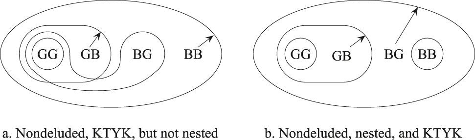
Non-deluded, KTYK, and nested illustrated.
2 Decision Theory Without Partitions
Our purpose in this paper is to analyze decision-making and game theory in environments where information processing is subject to error. Consider the following canonical decision problem:
Let A be a set of possible actions. Let
Condition (1)
Condition (2) For all
This definition applies for any possibility correspondence, whether or not it is a partition. Notice both conditions (1) and (2) serve to limit choices to reflect the level of information. Condition (1) requires that the agent's action is a function of what he perceives, and condition (2) requires that the agent optimizes, taking his information at face value.
In the above definition the agent is effectively unaware that he is erring in his information processing. Given the information that the state of nature
In the above decision framework the agent does not completely understand the model. He also does not necessarily “know what he is doing.” If he knew his optimal plan
To illustrate the definition above we shall shortly present three examples which shall be of further use in later sections. At the same time we investigate the precise sense in which an agent who knows more but is boundedly rational may be worse off than if he knew less but was unboundedly rational.
A fundamental consequence of Bayesian decision making, and unbounded rationality, is that knowing more can never be disadvantageous. If
Condition (3)
It turns out that this property of Bayesian decisions is at the heart of the non-speculation literature. By allowing for less rational information processing it need no longer be the case that more knowledge is better.
In fact, one wonders if there are any general properties at all that can be proved outside the Bayesian framework. We shall show however that there are. Indeed the “more is better property” applies to a more general set of information correspondences than partitions.
Example 2.1 Let
Of course
Example 2.2 Let
Once again let the coarse partition be
Example 2.3 Let
In this case condition (3) holds. Observe also that if we changed the payoff at
In Examples 2.1 and 2.2, the agent was (ex ante) worse off knowing more because he did not process information coherently. In Example 2.3 the agent was not worse off, although he also did not process information correctly. In general we have:
Theorem 1.
Let
Conversely, suppose that
Proof The proof of the first half of the theorem proceeds by induction on the cardinality of
But now we can apply the induction hypothesis to
Finally, let us observe that if
We conclude this section by noting one important extension to decision theory that fits naturally into our framework. Let
Condition (1′)
Condition (2′a)
Condition (2′b) For all
This new formulation allows us to model the idea that agents take the face value of a message, and restrict their choices accordingly, without using the subtle content of the message (i. e., without using knowledge of the function
Corollary 1.1
Let
Proof The proof is exactly as for Theorem 1.
3 Equivalent Decision Problems
Evidently the naming of states is somewhat arbitrary. For example, splitting a state into two indistinguishable states, which are physically identical but each with half the probability, should not change the decision problem. By formulating several definitions of equivalent decision problems we can clarify the framework of Section 2.
Definition We say that the decision problem
Decision-theoretic, if there is a 1–1 and onto map
Physical, if there is a function
We say that two decision problems are equivalent (in either of the two senses) if they have a common renaming. An easy argument shows that these are indeed equivalence relations, and that a physical renaming is also a decision-theoretic renaming.
The decision theoretic equivalence notion was formulated by Brandenburger, Dekel, and Geanakoplos 1992. If it holds and if agents always optimize according to (1) and (2), then behaviorally the decision problems are equivalent. The following lemma also appears in (Brandenburger, Dekel, and Geanakoplos 1992):
Lemma 1
For any decision problem
Sketch of Proof Let
The upshot of Lemma 1 is that we can understand the information processing and decision problem of Section 2 as
if the agent is a conventional maximizer, but has got the prior (on
The lemma thus provides us with another interpretation of decision theory with generalized partitions. If the reader wished, he could rewrite all of our results in terms of the consequences of using the wrong priors (or in later sections, of players using different priors). The advantage of the generalized possibility approach is that it explains how the mistaken priors might have arisen. Theorem 1, for example, gives conditions under which the agent does at least as well as he would with the right priors but less information. One perhaps could reformulate the result directly in terms of priors, but nondelusion, KTYK, and nested make clear just what information processing errors are tolerable.
We illustrate Lemma 1 with the ozone example in which
Let us now introduce the idea of a particularly simple, concrete description of the set of states of nature. Let us call
Notice that so far the ordering of the propositions has not played an essential role in our definitions. We suggest that a property of memory is that the propositions (or basic propositional events) are arranged in some definite order in the mind, perhaps from most important to least important, or reverse chronologically from most recent to most distant, so that one remembers the outcomes in order. Sometimes one might remember more or less (perhaps depending on the complexity of the outcomes), but always in the same order. More precisely:
Definition Let
We now show that nested can always be interpreted in terms of memory.
Lemma 2
Let
Proof The proof proceeds by induction on
Suppose now that the lemma is true for
Clearly, if
4 Game Theory with Generalized Partitions
We can extend game theory, as well as decision theory, to allow for information processing errors. The fundamental notion in game theory is the equilibrium concept provided by John Nash in 1951. Let
For all
We can interpret our definition of Nash equilibrium in much the same way as we did the single agent decision-maker. The players with non-partional Pi do not completely understand the model, and so they are led to make information processing blunders concerning the signals they receive.
One consequence of this point of view is that one of the rationalizations for Nash equilibrium, that each player deduces what he should do as a matter of logical introspection, is no longer tenable. However, many of the other interpretations of equilibrium are still viable. For example, an equilibrium can still be characterized as an agreement from which no agent has an incentive to deviate.
Let us emphasize one limitation of the current model. Agents are permitted to make errors about the significance of their signals. But these errors do not depend on the moves of other agents, even though, for example, the news that some state has occurred might be much more unpleasant depending on what the other players plan to do in that state. If we extended our equilibrium notion to allow for correlated equilibria, as in (Brandenburger, Dekel, and Geanakoplos 1992), then it would be natural to allow the errors to depend on the moves of other agents. (e. g., there might be some things that you simply refuse to believe somebody else would ever do.)
We now give three examples illustrating the definition of Nash equilibrium with generalized partitions, which will also serve to introduce the idea of speculation.
Example 4.1 Let
where
Example 4.2 Let
where
Example 4.3 Let
where
If we changed the payoff at
We might consider a third variant of the game in which the payoffs are as in the second variant, but now
We now show that Nash equilibrium with generalized partitions can always be given a Bayesian interpretation.
Definition We say that the game
The following lemma appears in (Brandenburger, Dekel, and Geanakoplos 1992).
Lemma 3
Any generalized game
Proof Let
for
As an immediate corollary we have
Theorem 2
If the action spaces
Proof There is always a decision-theoretic renaming
5 Necessary and Sufficient Conditions for Speculation in Equilibrium
Will rational, risk averse agents bet against each other? Might they speculate against each other if it is not common knowledge how much each agent is betting? Can they agree to disagree about the probability of some event? What if they have access to different information? What if some of them make information processing errors?
Aumann (1976) showed that when agents have partition knowledge, it cannot be common knowledge that they disagree. Milgrom and Stokey (1983), and less generally Sebenius and Geanakoplos (1983), showed that when agents have partition knowledge, it cannot be common knowledge that they will speculate or bet against each other. Finally, a number of authors, in a long series of papers, have shown that even without common knowledge of all the individual actions, there can be no speculation in a rational expectations equilibrium (e. g., Kreps 1977; Tirole 1982). With partition-information all of these theorems are pretty much the same: they can all be instantly derived from one theorem which we shall give below. When knowledge is described by generalized partitions, however, these theorems are distinct; their proofs are different and so are the hypotheses needed for each of them.
Speculation, betting, and disagreement can all be described in terms of Nash equilibrium. Examples 4.1 and 4.2 show that speculation and betting can occur in Nash equilibrium if the possibility correspondences
On the other hand, perhaps it is not surprising that agents can bet against each other, even though they have common priors, when their rationality is bounded. After all, one way such generalized partitions can arise is if the agents are faulty in their processing of information. For example, they may ignore all unfavorable information. Another way to see the same thing, as the proof of Lemma 3 makes clear, is that a generalized equilibrium is isomorphic to a Bayesian partition equilibrium in which the priors may be different. The agents may have started with common priors, but on account of their faulty information processing, they behave as if their priors were different. It is well-known that gambling can take place between agents with different priors.
In this light the surprise is that any weakening of partition information still retains enough structure to prevent speculation. Recall for instance that nondelusion, knowing that you know, and nested are together still consistent with throwing away unpleasant information at least once. Yet we have: all agents nondeluded, nested, and KTYK ⇔ no equilibrium speculation. The following theorem represents nonspeculation as strategies zi that lead to certain payoffs that cannot be Pareto dominated. Speculation occurs when agents depart from zi .
Theorem 3
Let
Proof Let
In Example 4.1 speculation occurs because
The examples show that KTYK, nondeluded, and nested not only suffice to eliminate speculation in Nash equilibrium, but are necessary as well. If an agent's information
Like Theorem 1, Theorem 3 can be extended to allow for variable action spaces.
Corollary 3.1
Consider the generalized game
Proof Follow the logic of the proof of Theorem 3, and apply Corollary 1.1 where
We can immediately apply the above theorem to show a generalization of the standard no speculation theorem in rational expectations equilibrium.
We define an economy
Definition A rational expectations equilibrium (REE)
Let
The reference to rational in rational expectations equilibrium comes from the fact that agents use the subtle information conveyed by prices in making their decisions. That is, they not only use the prices to calculate their budgets, they also use their knowledge of the function p to learn more about the state of nature. If we modified (iii) and (iv) above to
Then we would have the conventional definition of competitive equilibrium (CE). The following nonspeculation theorem holds for REE, but not for CE. [For proofs when agents have partition information and learn from prices, see Dubey, Geanakoplos, and Shubik 1987; Kreps 1977; Tirole 1982.] For an example with partition information in which agents do not learn from prices, and so speculate, see Dubey et al. (1987). We say that there are only speculative reasons to trade in E if in the absence of asymmetric information there would be no perceived gains to trade. This occurs when the initial endowment allocation is ex ante Pareto optimal, that is if
Corollary 3.2
Let
Proof The proof follows immediately from Corollary 3.1. Let
6 Knowing Your Own Action
Consider again the single person decision problem
Recall that in decision theory, the agent begins with a prior π on
The agent always knows what he is doing under the action plan f if the action he is supposed to take is always self-evident to him. We shall describe the circumstances in which an agent who “always knows what he is doing” may appear to be perfectly rational even when he is making information processing errors.
Definition An agent who processes information according to
We shall now show that if an agent always knows what he is doing (i. e., knows for all
Definition The information processor
If the same holds true for some λ unrestricted in sign,
Balancedness gives a condition under which one can say that every element
There is a special class of events for which being balanced is especially important. Recall:
Definition An event
Definition
If
We now use the notion of self-evident events to characterize the relationship between positively balanced and balanced and nondeluded, KTYK, and nested. Positively balanced is a weakening of nested, and balanced is a further weakening that is also a weakening of KTYK.
Lemma 4
If
Proof Let E be self-evident to
Lemma 5
Let
Proof The proof proceeds by induction. If
In later sections we show that if each agent is nondeluded, then
all agents balanced
all agents positively balanced
As a prelude to demonstrating these two equivalences, in our next theorem we show that Theorem 1 can be proved under much weaker hypotheses if we suppose that the agent knows what he is doing. (Needless to say, if an agent is not unboundedly rational, we might not expect him always to know what he is doing.)
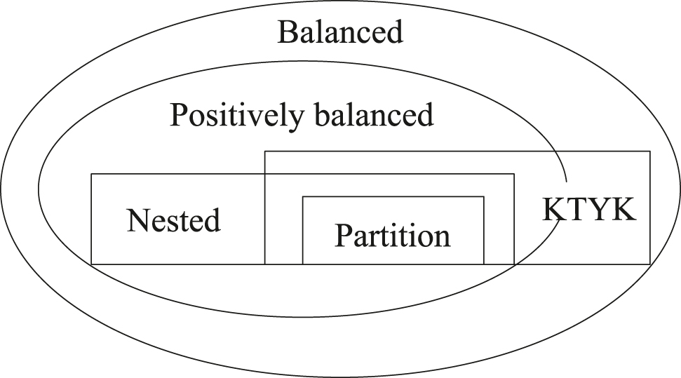
The logical connections between balanced, positively balanced, nested, KTYK, and partition information, assuming nondeluded.
Theorem 4
Let
If
Proof Since
Let E ∈
Q
. Since
Q
is a partition of
By nondelusion, if
But for any
To argue in the other direction, note that there are trivial counterexamples if
The idea behind the proof of Theorem 4 is quite different from that used in the proof of Theorem 1. The following definitions are clarifying.
Definition A function
Behavior which is optimal in the sense we have described, where information processing errors are represented by possibility correspondences or generalized partitions, always satisfies the generalized sure-thing principle.
Theorem 4 has one particularly important consequence. Suppose an agent who is nondeluded and positively balanced optimally chooses some action plan f under which he knows what he is doing. If the agent were to forget everything he knew except what was necessary to implement the decision plan, then he would still choose the same plan. To put the matter still differently, the optimal behavior of an agent who is nondeluded and positively balanced and always knows what he is doing cannot be distinguished from the behavior of an unboundedly rational (partition information processing agent).
7 Common Knowledge of Events vs. Common Knowledge of Actions
Aumann (1976) introduced the idea of common knowledge of events and actions. We investigate what conclusions we can draw (about speculation and consensus) when we add the additional hypothesis that actions are common knowledge. Again we find a nonspeculation theorem, but under weaker conditions than Theorem 4, and with a different proof. We also derive a consensus theorem under still weaker hypotheses, with yet another kind of proof.
We can already get some idea of the importance of the hypothesis that actions are common knowledge from Example 4.2. The agents do bet in equilibrium, but at the moment each commits himself to the bet he does not know whether it will be accepted or not. The bet is not common knowledge. We now formalize this idea.
The possibility correspondence
If
Definition (Lewis (1969), Aumann (1976)) We say that an event A is “common knowledge at ω” if for any n, and any sequence of players
We can give an equivalent definition of common knowledge based on our familiar notion of self-evident event.
Definition Let agents' knowledge be represented by
The following proposition is taken from Brown and Geanakoplos (1988), or Monderer and Samet (1988), extending Shin (1987), who extended Aumann (1976). The reader interested in a further discussion of common knowledge is referred to any of these works.
Proposition Let the knowledge of agents
Not only events, but also actions can be common knowledge.
Definition Let
Observe that if f is the action plan of some player i, then one consequence of f being common knowledge at ω is that i himself knows what he is doing at ω. Replacing
There would seem to be a wide gulf between the hypothesis that agents know the same things (about all events) and the hypothesis that agents know the same things about what they are each planning to do. Indeed it is commonly held that we observe agents interacting (i. e., taking actions) in various ways on account of the fact that they have asymmetric information. The following theorem, however, describes the power of assuming actions are common knowledge. It generalizes a theorem (Geanakoplos, 1987), proved for Nash equilibria, following an idea in Cave (1983). It shows that if in Nash equilibrium the actions are common knowledge at ω, then the information might as well be the same as well. Hence once actions are presumed to be common knowledge, asymmetric information provides no explanation whatsoever of behavior.
Theorem 5
Let
Proof From the proposition we know that there is a public event E such that
The hypotheses in Theorem 5 are not only sufficient for Theorem 5, but necessary as well. If some agent's information processing
8 Necessary and Sufficient Conditions for Common Knowledge Speculation
Corollary 5.1
Consider the speculative situation of Theorem 3. Drop the assumption that agents know what they know and are nested. Suppose only that
Proof From the common knowledge hypothesis, for each i, there is a
From this it follows that the ex ante payoffs to each player from the moves
would be at least
Corollary 5.2
Let
9 Necessary and Sufficient Conditions to Agree to Disagree
A game of particular interest is the opinion game
Theorem 6
Suppose that in the generalized opinion game
Proof From nondelusion and balancedness, for any public event E we can write
Using nondelusion and balancedness,
or
The converse follows from Farkas' Lemma as in the proof of Theorem 4, except since all the inequalities are equalities here, the
Aumann (1976) gave the first famous version of this theorem, for partitions. (Geanakoplos and Polemarchakis 1982) gave a dynamic version of the same theorem. Samet (1987) showed that as long as each
McKelvey and Page (1986) proved the remarkable theorem that if the average (or sum) of different agents' opinions is common knowledge and if each agent began with the same prior, all the opinions must be the same. For another proof see (Brandenburger et al. 1990). Here we extend this result to possibility correspondences satisfying only nondeluded, nested, and knowing that you know. The proof can also be regarded as an alternative derivation of McKelvey-Page's average opinion theorem.[4]
Theorem 7 Suppose that in the generalized opinion game
Proof Since
Observe that from Theorem 1 and the fact that
Multiplying out terms and noting that
Subtracting
unless
10 Generalized Games in Extensive Form
Let us now apply our theory to games in extensive form. In this theory players act over time, and in particular the same player may move many times. The inconsistency that occurs when information is not given by partitions and total recall can now reveal itself in time inconsistency of behavior.
Consider a tree, consisting of a finite set of nodes
To every node ω we associate a possibility set
A strategy for a player i is an association with each
Given the strategies
To each
We define an equilibrium, for the generalized game G as a tuple of strategies
Theorem 8 Every generalized game in extensive form has an equilibrium.
Here is not the place to go into details, but one can also define various refinements of equilibrium for generalized games. A perfect equilibrium for a generalized game in extensive form can be defined analogously to a perfect equilibrium for a conventional game in extensive form, since in the latter case one must appeal also to the agent normal form.
One could give many examples of generalized games in extensive form, but let us concentrate on the story of Odysseus and the Sirens, and the problem of time consistency.
Recall that one day Odysseus was told by Circe that his boat would be sailing near the island home of the famous Sirens, whose beautiful singing lured many sailors to crash against the terrible rocks that studded the shore. Anticipating that once they heard the music, he and his men would not be able to resist the seductive temptation to sail nearer to the shore to better hear the songs, he ordered his men to sail clear of the shore, and he put wax in their ears to make sure that they could hear neither the Sirens nor himself. He also had himself tied to the mast, so that he could hear the Sirens but could do nothing to change the course of the boat. When the boat finally came within earshot of the Sirens, Odysseus struggled violently to free himself from his bonds and to exhort his men toward shore. Fortunately for him, both the wax and the bonds held firm, and his boat sailed safely past.
Odysseus' decision problem is one of the best known in history, precisely because Odysseus is so famous for his cunning, which indeed this story seems to confirm, and yet his behavior before and after hearing the Sirens is apparently inconsistent. A celebrated explanation, given by (Strotz, 1955), suggests that Odysseus was a man who greatly discounted the future, but did not discount the distant future much more than the near future. According to this theory, when Odysseus first realized where he was, he weighed the near future of sailing near shore to better hear the sirens against the distant future of crashing on the rocks, and decided to avoid the bargain. But when the near future became the present, so that the trade-off was between hearing better now and crashing later, he wanted the bargain.
Although this impatience explanation is quite striking, it is not clear that it is faithful to the story, nor that it is the most interesting explanation. In the first place, one of the salient characteristics of Odysseus' personality is that, unlike most of the other Greeks, he was always planning for the future. These plans and preparations often involved initial sacrifices for future rewards. (Meticulously arranging the wax for his men is a perfect example.) It does not seem credible that wily Odysseus would trade his life for a song just because the song came first. (Indeed if anything he was willing to give up his life to the Trojan expedition in order to be part of the immortal song of the poet, because that song is last, and everlasting.) There is a further technical problem with Strotz's explanation, namely that it suggests discontinuous preferences. Until the moment Odysseus hears the song, he keeps his wits and tries to avoid the rocks. It is only at the instant that he hears the music that he forgets himself. This behavioral change cannot be accounted for by continuous time preferences, that ignore the information content of the song.
The theory of extensive form games proposed here is designed to model behavior that is purposeful and cunning, but based on information processing that is not perfect. My interpretation is that when Odysseus hears the Sirens and “forgets himself,” he literally forgets what he knew before, namely that the Sirens are dangerous. His behavior after he hears the Sirens is not less purposeful or less skillful than before. The difference is that it is constrained and it is based on different information. Typically such a beautiful song deserves a better hearing, and having forgotten the warning of Circe, Odysseus struggles to land his boat closer to shore. The subtlest part of this information explanation of Odysseus, and one that requires all of the apparatus of the model, is that Odysseus recognizes full well that he is ensnared in the ropes and cannot get the attention of his men. But he never asks himself how he got in that situation. If he did he might have inferred his predicament. Thus the information explanation, which I believe expresses the paradox of the inconsistent but cunning planner in a way which impatience cannot, rests on the two ideas which are the basis of our extension of game theory. Knowledge is not necessarily describable by partitions, and even the most clever men do not necessarily make inferences from the constraints they face.
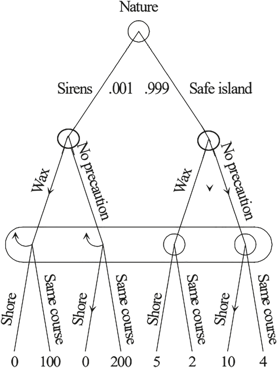
The Odysseus game can be formally modeled in our framework, as the following diagram makes clear. Nature moves first and chooses to blow Odysseus' boat near the island of the Sirens, or near some other harmless island (on which there is also singing, but perhaps less good). Odysseus then has the choice of binding himself and putting wax in the ears of his men, or else leaving them all free. Finally he hears the music, and must decide whether to give the order to stay clear of the shore, or to move toward the shore. Note that if he has put wax in his mens' ears, then he is constrained not to give the order to head closer to shore, although the payoff if he were able is still defined.
The novelty about this game is the information Odysseus has. Odysseus hears very well the advice of Circe, and so knows whether the boat will be sailing past the island of the Sirens or a harmless island. If he hears songs from the harmless island, he remembers well whether he put wax in the ears of his men. A best strategy from that point is to sail close to shore. But if Odysseus is near the Sirens' island, and hears their singing, then he forgets completely Circe's advice. Moreover, although he recognizes whether he is bound or not, he does not infer anything from this. See Figure 3.
There is a unique equilibrium to this generalized game in extensive form. Odysseus applies the wax if Circe advises him that he will pass the Sirens, and otherwise, he does not. After hearing either song, he always tries to head for shore, but when he is constrained from giving such an order he does the only thing he can, and permits the boat to stay clear. The reason this last move of Odysseus is optimal is because Odysseus computes that 99.9% of the time he is called upon to make a decision about whether to better hear a beautiful song, it is worth doing. Knowing that he will decide this way later, Odysseus earlier on has no choice but to put the wax in his mens' ears and tie himself to the mast, even though he would be much better off sailing clear of the island unfettered.
The time inconsistency of Odysseus' behavior is mirrored in a host of similar examples usually having to do with temptation. Typically the optimal response to a pleasant sensation is to increase it. Life's experiences strongly encourage such priors. There are some pleasant experiences, like some drugs or cigarette smoking that some people recognize to be harmful for them. However, when under their influence, or sometimes just in their presence, they forget the particular, and reason only from the general principle that pleasure is desirable. One occasionally meets modern day Odysseuses who deliberately leave their money home so they will not be tempted by anything fattening, or who join clubs like alcoholics anonymous so that their drinking will be punished by shame as well as hangovers.
The generalized partition that makes Odysseus an optimizer with standard discounting.
References
Aumann, R. 1976. “Agreeing to Disagree.” The Annals of Statistics 4: 1236–39, https://doi.org/10.1214/aos/1176343654.Search in Google Scholar
Bacharach, M. 1985. “Some extensions of a claim of Aumann in an axiomatic model of knowledge.” Journal of Economic Theory 37: 167–90, https://doi.org/10.1016/0022-0531(85)90035-3.Search in Google Scholar
Brandenburger, A., E. Dekel, and J. Geanakoplos. 1992. Correlated Equilibrium with Generalized Information Structures, 4, 182–201. Games and Economic Behavior. https://doi.org/10.1016/0899-8256(92)90014-J.Search in Google Scholar
Brandenburger, A., J. Geanakoplos, R. McKelvey, L. Nielson, and T. Page. 1990. “Common Knowledge of an Aggregate of Expectations.” Econometrica 58: 1235–9, https://doi.org/10.2307/2938308.10.2307/2938308Search in Google Scholar
Brown, D., and J. Geanakoplos. 1988. Common Knowledge without Partitions. Unpublished.Search in Google Scholar
Cave, J. 1983. “Learning to Agree.” Economic Letters 12: 147–52, https://doi.org/10.1016/0165-1765(83)90126-x.Search in Google Scholar
Doyle, Arthur Conan. 1901. The Adventure of Silver Blaze: The Strand Magazine.Search in Google Scholar
Dubey, P., J. Geanakoplos, and M. Shubik. 1987. “The Revelation of Information in Strategic Market Games: A Critique of Rational Expectations Equilibrium.” Journal of Mathematical Economics 16(2): 105–38, https://doi.org/10.1016/0304-4068(87)90002-4.Search in Google Scholar
Geanakoplos, J. 1987. Common Knowledge of Actions Negates Asymmetric Information: mimeo, Yale University.Search in Google Scholar
Geanakoplos, J. 1988. Common Knowledge, Bayesian Learning, and Market Speculation with Bounded Rationality: mimeo, Yale University.Search in Google Scholar
Geanakoplos, J., and H. Polemarchakis. 1982. “We Can’t Disagree Forever.” Journal of Economic Theory 28 (1): 192–200, https://doi.org/10.1016/0022-0531(82)90099-0.Search in Google Scholar
Kreps, D. 1977. “A Note on Fulfilled Expectations Equilibrium.” Journal of Economic Theory 14 (1): 32–43, https://doi.org/10.1016/0022-0531(77)90083-7.Search in Google Scholar
Lewis, D. 1969. Conventions: A Philosophical Study. Cambridge: Harvard University Press.Search in Google Scholar
McKelvey, R., and T. Page. 1986. “Common Knowledge, Consensus, and Aggregate Information.” Econometrica 54: 109–27, https://doi.org/10.2307/1914160.Search in Google Scholar
Milgrom, P., and N. Stokey. 1982. “Information, Trade, and Common Knowledge.” Journal of Economic Theory 26: 17–27, https://doi.org/10.1016/0022-0531(82)90046-1.Search in Google Scholar
Monderer, D., and D. Samet. 1988. Approximating Common Knowledge with Common Beliefs, 1, 2nd ed., 170–190. The Journal of Games and Economic Behavior. https://doi.org/10.1016/0899-8256(89)90017-1.Search in Google Scholar
Samet, D. 1987. Ignoring Ignorance and Agreeing to Disagree. MEDS Discussion Paper: Northwestern University.Search in Google Scholar
Sebenius, J., and J. Geanakoplos. 1983. “Don’t Bet On It: Contingent Agreements with Asymmetric Information.” Journal of the American Statistical Association 78: 424–6, https://doi.org/10.1080/01621459.1983.10477988.Search in Google Scholar
Shin, H. 1987. Logical Structure of Common Knowledge, I and II. unpublished. Oxford: Nuffield College.Search in Google Scholar
Strotz, R. H. 1955–6. “Myopia and Inconsistency in Dynamic Utility Maximization.” Review of Economic Studies 23: 165–80, https://doi.org/10.2307/2295722.Search in Google Scholar
Tirole, J. 1982. “On the Possibility of Speculation under Rational Expectations.” Econometrica 50 (5): 1163–81, https://doi.org/10.2307/1911868.Search in Google Scholar
© 2020 Walter de Gruyter GmbH, Berlin/Boston
Articles in the same Issue
- Frontmatter
- Special Issue on Unawareness
- Editorial
- Introduction to the Special Issue on Unawareness
- Research Articles
- Game Theory Without Partitions, and Applications to Speculation and Consensus
- Do I Know Ω? An Axiomatic Model of Awareness and Knowledge
- Games with Unawareness
- Knowledge, Awareness and Probabilistic Beliefs
- Prudent Rationalizability in Generalized Extensive-form Games with Unawareness
- Reverse Bayesianism: A Generalization
- Ambiguity and Awareness: A Coherent Multiple Priors Model
- Updating Awareness and Information Aggregation
- Delegation and Information Disclosure with Unforeseen Contingencies