College Assignment Problems Under Constrained Choice, Private Preferences, and Risk Aversion

Allan Hernandez-Chanto

doi:10.1515/bejte-2019-0002

Enjoy 40% off

academic books on De Gruyter Brill *

Article

College Assignment Problems Under Constrained Choice, Private Preferences, and Risk Aversion

Allan Hernandez-Chanto

Published/Copyright: February 19, 2020

Published by

Become an author with De Gruyter Brill

Submit Manuscript Author Information Explore this Subject

From the journal The B.E. Journal of Theoretical Economics Volume 20 Issue 2

Abstract

Many countries use a centralized admission system for admitting students to universities. Typically, each student reports a ranking of his preferred colleges to a planner, and the planner allocates students to colleges according to the rules of a predefined mechanism. A recurrent feature in these admission systems is that students are constrained in the number of colleges that they can rank. In addition, students normally have private preferences over colleges and are risk-averse. Hence, they face a strategic decision under uncertainty to determine their optimal reports to the planner. We characterize students’ equilibrium behavior when the planner uses a Serial Dictatorship (SD) mechanism by solving an endogenous decision problem. We show that if students are sufficiently risk-averse, their optimal strategy is to truthfully report the “portfolio of colleges” with the highest probabilities of being available. We then analyze the welfare implications of constraining student choice by stressing the differences between the so-called consideration and conditional-allocation effects.

Keywords: college assignment; conditional-alloation effect; consideration effect; constrained choice; private preferences; risk aversion

JEL Classification: D47; D60; D81

Acknowledgements

A previous version of the manuscript circulated under the title “On the Optimality of Constrained Choice in College Assignment Problems.” I am indebted to Amanda Friedenberg for stimulating conversations and advice. I am also thankful to Andres Fioriti and Alejandro Manelli for their comments. All errors are my own.

Appendix

A Omitted Proofs

Proof of Proposition 2

Fix a student s ≤ K. Notice that for any type vs and any belief about the strategy profile of other students, reporting the K-most-preferred colleges is a best response for student s. We have to show that for any non-truthful strategy σˆs, there exists a profile of strategies played by the other students, such that submitting a report according to σˆs is non-optimal.

Now, fix an index 2≤ℓ≤s≤K, and let V=(v1,…,vS) be a profile of students’ types such that π(j|vs′)=π(j|vs) for all s' < s and all j=1,…,ℓ−1. That is, the type of all students with strictly higher priority than s rank the first ℓ−1 colleges in the same way as the type of student s. Such a profile of types has strict positive probability.

Let σ−s be such that σs′(vs′)=rs′, with rs′,j=π(j|vs′) for all s' < s and all j = 1, …, K. In other words, students with strict higher priority than s report truthfully up to the Kth-most-preferred college. In turn, let student s report according to the strategy σˆs(vs)=rs, such that:

(14)rs,j=π(j|vs)∀j<ℓπ(h|vs)forj=ℓand someh>ℓ

Under this strategy, student s will be assigned to his hth-preferred college, whereas if he truthfully reports his preferences he would be assigned to his ℓth-preferred college.

Proof of Proposition 3

By Proposition 2, all students with priority greater than K are K-truthful. Now, consider the student K + 1—i. e. the marginal student. He can compute his vector of ex-ante admission probabilities γK+1(σ−(K+1)∗) from the distribution of preferences drawn by the students with higher priority. This is sufficient because there is no uncertainty about the strategies played by his predecessors. Given these admission probabilities and his preference type vK+1, he can solve the decision problem (EDP) to determine his optimal response σK+1∗. Student K + 2 can proceed analogously to solve his corresponding EDP. Now, he has to consider the strategy σK+1∗ of his immediate predecessor at the time of computing his vector of admission probabilities γK+2∗(σ−(K+2)∗). This is so because student K + 1 is not necessarily K-truthful. We can proceed by induction to determine the optimal strategy of all students with lower priority.

Proof of Proposition 4

Each student s with priority lower than K (i. e. such that s > K) solves the corresponding problem stated in the equation (EDP), given his vector of admission probabilities and his vector of cardinal utilities.

Let ΓsK(σ−s∗) be the set of his K colleges with the highest probability of admission.^[13] Notice that for any student s, the set of colleges C can always be partitioned into a set of “least-preferred colleges” and a set of “most-preferred colleges” because cardinal preferences are strict. Hence, by Theorem 1 in Chade and Smith (2006), we can use the Marginal Improvement Algorithm (MIA) to find the solution of each student’s combinatorial problem. MIA is a greedy algorithm that looks for the option that yields the highest marginal increment in the expected utility at each stage. Specifically, in the first stage, it chooses the college that yields the largest expected utility, and then, in step ℓ≥2, it selects the option that yields the largest marginal benefit over the portfolio of colleges constructed so far.^[14]

For any vs∈V, and a given ρ∈R+, define

rs,1(vs,ρ)=argmax{u(c,vs,ρ)γs(c|σ−s∗),c∈C}

Then, there exists a sufficiently high level of risk aversion ρs,1(vs), such that, rs,1(vs,ρs,1(v˙s))∈ΓsK(σ−s∗). Indeed, fix c∈ΓsK(σ−s∗), and notice that for any c′∈C∖ΓsK(σ−s∗),

Δ(c,c′|σ−s∗)=γs(c|σ−s∗)γs(c′|σ−s∗)>1

Hence, because the utility function u(⋅,vs,ρ) is concave, with a concavity degree parameterized by ρ, there exists a level of risk aversion ρs,1(vs) such that

u(c′,vs,ρs,1(vs))u(c,vs,ρs,1(vs))<Δ(c,c′|σ−s∗)

In the same fashion, define inductively,

rs,j(vs,ρ)=argmax{u(c,vs,ρ)γs(c|σ−s∗),c∈C∖{rs,1(vs,ρ(vs)),…,rs,j−1(vs,ρ(vs))}}

for j = 2, …, K.

Following the same argument as before, we can find a sufficiently high level of risk aversion ρs,j(vs), such that, rs,j(vs,ρs,j(vs))∈ΓsK(σ−s∗)∖{rs,1(vs,ρ(vs)),…,rs,j−1(vs,ρ(vs))}. Thus, there would be a collection of risk-aversion parameters, such that the optimal portfolio consists of the K colleges with higher probability of admission. Then, take

ρs(vs)=max{ρs,1(vs),…,ρs,K(vs)}

Next, let

ρs=max{ρs(vs):vs∈V}

Therefore, if ρ ≥ max{ρ_s : s > K}, the optimal strategy for those students for which the constraint binds is to choose the K colleges with maximal probability of admission.

Finally, note that the constrained SD is equivalent to the constrained deferred acceptance mechanism when colleges rank all students in the same way (i. e. when priorities are uniform). Then, we can use result (ii) in Proposition 4.2 in Haeringer and Klijn (2009) to conclude that a constrained student can do no better than to rank the selected colleges in his “portfolio” according to his true preferences.

Proof of Proposition 5

Suppose that the number of options to report K is such that |Γs(σ−s∗)|<K for all s > K—i. e. for all students with priority lower than K. Then, the best strategy for those students is to report all the colleges with positive probability according to their true type. Meanwhile, the best strategy for students with priority higher than K is to be K-truthful. Hence, there is no change in the equilibrium allocation with respect to the unconstrained case, which is a contradiction.

Proof of Proposition 6

Fix 1 < K < C. Let η^k(c) be the ex-ante probability that college c is the kth most preferred college. That is,

ηk(c)=∑v∈V\mathds1{π(k|v)=c}Pr(v).

Write η(c)=(ηk(c):k=1,…,C) as the distribution of college c in the spectrum of preferences.

Recall that for each student s, and each strategy profile σ=(σs:s∈S),γs(σ)=(γs(c|σ−s):c∈C) corresponds to the vector of college-available probabilities. By Proposition 3, we have that γs(σ∗)=γs(ξ∗) for any student s ≤ K + 1. Furthermore, because all students s ≤ K report truthfully both in the constrained and the unconstrained mechanism, we have that for any two colleges c≠c˜,

∑k=1tηk(c)≥∑k=1tηk(c˜)fort=1…,C⇒γK+1(c|σ−(K+1)∗)≤γK+1(c˜|σ−(K+1)∗)∑k=1tηk(c)≥∑k=1tηk(c˜)fort=1,…,C⇒γK+1(c|ξ−(K+1)∗)≤γK+1(c˜|ξ−(K+1)∗).

Now, following Proposition 3, in the constrained mechanism, student K + 1 chooses the colleges with K-highest probabilities of being available, ΓK+1K(σ−(K+1)∗). Hence, for all c∈ΓK+1K(σ−(K+1)∗) and c˜∈C∖ΓK+1K(σ−(K+1)∗) we have that:

∑k=C−K+1Cηk(c)≥∑k=C−K+1Cηk(c˜).

In contrast, in the unconstrained mechanism student K + 1 reports truthfully, and, thus, if the student chooses to report college c and not to report college c˜, we have that:

∑k=1Kηk(c)≥∑k=1Kηk(c˜).

Therefore, γ(σK+2∗) ex-ante dominates γ(ξK+2∗). We can proceed inductively for all students s ≥ K + 2 to conduct the same analysis.

B Equilibrium in the DA and TTC

In this section, we discuss the extent to which our analysis of the student’s behavior in the SD mechanism can be carried over to the Deferred Acceptance (DA) and Top-trading Cycles (TTC) mechanisms. The DA and the TTC were introduced by Abdulkadiroğlu and Sönmez (2003) to study the assignment of students to elementary schools in admission procedures whereby students report preferences over schools, and schools prioritize students differently based on criteria of proximity and sibling precedence at the school. When preferences and priorities are common knowledge and students are not constrained in the number of options that they can report, both mechanisms have desirable properties that make them attractive for policy makers. In particular, the DA is strategy-proof and stable, although not Pareto-efficient, whereas the TTC is strategy-proof and Pareto-efficient, although not stable. If students are constrained in their choice, but preferences and priorities continue to be common knowledge, Haeringer and Klijn (2009) show that neither the DA nor the TTC is strategy-proof. Furthermore, the DA ceases to be stable, while the TTC ceases to be efficient. However, stability in the DA can be restored if the priority structure satisfies the Ergin (2002) acyclicity condition, whereas efficiency in the TTC can be restored if the priority structure satisfies the X-acyclicity condition—see Haeringer and Klijn (2009). When students are constrained in their choice, and preferences are private information, the DA and the TTC cease to exhibit all their desirable properties. Furthermore, students’ decision problem becomes complex, as they might have different priorities for all schools and have to form beliefs over other students’ preferences and strategies to determine their best response. We discuss the challenges of implementing our equilibrium characterization in the DA and the TTC.

Deferred Acceptance The Deferred Acceptance mechanism is based on the pioneering work of Gale and Shapley (1962). It is the most commonly used mechanism in matching environments, ranging from the matching of students with elementary schools to the matching of residents with hospitals. The description of the algorithm in the college assignment problem when students propose their preferred options is as follows:

Step 1: Each student proposes his first choice. Each college tentatively assigns its seats to its proposing students following their priority order. Any remaining proposers are rejected.
Step ℓ≥2: Each student who was rejected in the previous step proposes her next choice. Each college considers the students that were tentatively assigned in the previous step, along with its new proposers, and tentatively assigns its seats to those students following their priority order. Any remaining proposers are rejected.
The algorithm terminates when no student’s proposal is rejected and all tentative assignments become final assignments.

As Agarwal and Somaini (2018) demonstrate for the school choice problem, the equilibrium in the DA can be characterized by computing a vector of cutoff values—i. e. a vector of minimum priority orders necessary to get a seat in each school. Analogously, the equilibrium of the college assignment problem can be characterized by computing a vector of threshold scores. Here, a threshold score for each college c corresponds to the lowest admission score obtained by some student s assigned by the mechanism to such a college. Following Balinski and Sönmez (1999), let Z={z1,…,zN} be a list of skill categories evaluated in the admission test, and denote xs=(xs(z1),…xs(zN))∈XN as the student s’s vector of scores in each category. Furthermore, let ζ:C→Z be the function that determines the relevant test category used by each college to prioritize students. Now, fix an arbitrary student s. For each profile of reports R−s=(rs˜:s˜∈S∖{s}), and each profile of scores X−s=(xs˜:s˜∈S∖{s}), the threshold score of college c when student s is absent from the mechanism is defined by the function τˆ−sc:RS−1×XS−1→T⊂X such that^[15]:

τˆ−sc(R−s,X−s)=min{xs˜(ζ(c))∈X:ψˆs˜K(R−s,X−s)=c,s˜∈S∖{s}}∀c∈C.

Hence, using the same notation as in Section 4, we have that:

γs(c|σ−s,X−s)=∑VS−1∈VS−1\mathds1{xs(ζ(c))>τˆ−sc(σ−s(V−s),X−s)}Pr(V−s).

That is, the probability that college c is available to student s is equal to the probability that the student’s admission score in the category relevant to c, x_s(ζ(c)), is higher than the endogenous threshold score in such a college.

Hence, given a vector of college-available probabilities γs(σ−s)=(γs(c|σ−s):c∈C), and a preference type vs, each student s can solve the corresponding endogenous decision problem stated in (EDP). However, because students’ priorities are multidimensional and, thus, cannot be totally ordered, there is no hierarchical structure over the college-available probabilities. Therefore, we cannot use the same analysis as in Section 5 to derive the welfare equilibrium implications of students’ behavior when they are risk-averse and face uncertainty over assignments.

Top-Trading Cycles The Top-trading Cycles mechanism was proposed by Shapley and Scarf (1974) and adopted by Abdulkadiroğlu and Sönmez (2003) as a competing mechanism to the DA in the school choice problem. The essence of the mechanism is to allow students with high priorities to trade their assignments to facilitate Pareto improvements. The main advantage of TTC is that it eliminates all possible inefficiencies. However, it does so at the expense of not eliminating all students’ justified envy. The description of the algorithm is as follows:

Step 1: Assign a counter for each college to keep track of how many seats are still available at that particular college. Initially, set the counters equal to the capacities of the colleges. Each student points to his favorite college under his announced preferences. Each college points to the student who has the highest priority for the college. The set of students and colleges that point to some other element in the set form a cycle. Hence, a cycle can be represented as an ordered list of distinct colleges and students—i. e. (s1,c1,…sℓ,cℓ). Every student in a cycle is assigned a seat at the college he points to and is removed. The counter of each college in a cycle is reduced by one, and if it reduces to zero, the college is also removed. The counters of all other colleges become the initial capacities for the next iteration.
Step ℓ≥2: Each remaining student points to his favorite college among the remaining colleges, and each remaining college points to the student with the highest priority among the remaining students. Every student in a cycle is assigned a seat at the college he points to and is removed. The counter of each college in a cycle is reduced by one, and if it reduces to zero, the college is also removed. The counters of all other colleges become the initial capacities for the next iteration.
The algorithm terminates when either the reports of all students have been considered or all the seats have been assigned.

Unlike the DA, the equilibrium of the TTC cannot be characterized by a series of threshold scores, and, thus, the computation of the college-available probabilities is substantially more complicated. To illustrate this, notice that if a student s does not have the highest priority in college c, but has the highest priority in college c˜, there must exist a cycle in which a student s˜ points to college c˜, so it entitles student s a seat in college c. Now, if student s is not assigned in the first iteration of the algorithm, the same analysis should be in place for the rest of the iterations. Therefore, to compute the availability of a college under the same strategy profile, the same analysis should be conducted for each possible cycle induced by students’ strategies and preferences. As before, even if we were able to characterize students’ equilibrium behavior following a portfolio approach, it is not possible to determine the welfare implications of students’ choices.

C Additional Graphs

Figure 6:

College-available probabilities for all ranked choices. The figure shows the average college-available probabilities for each kth-preferred college. Fixing ρ = 1, panels (Figure 6a)–(Figure 6d) vary the probability of drawing the pivotal type p.

Figure 7:

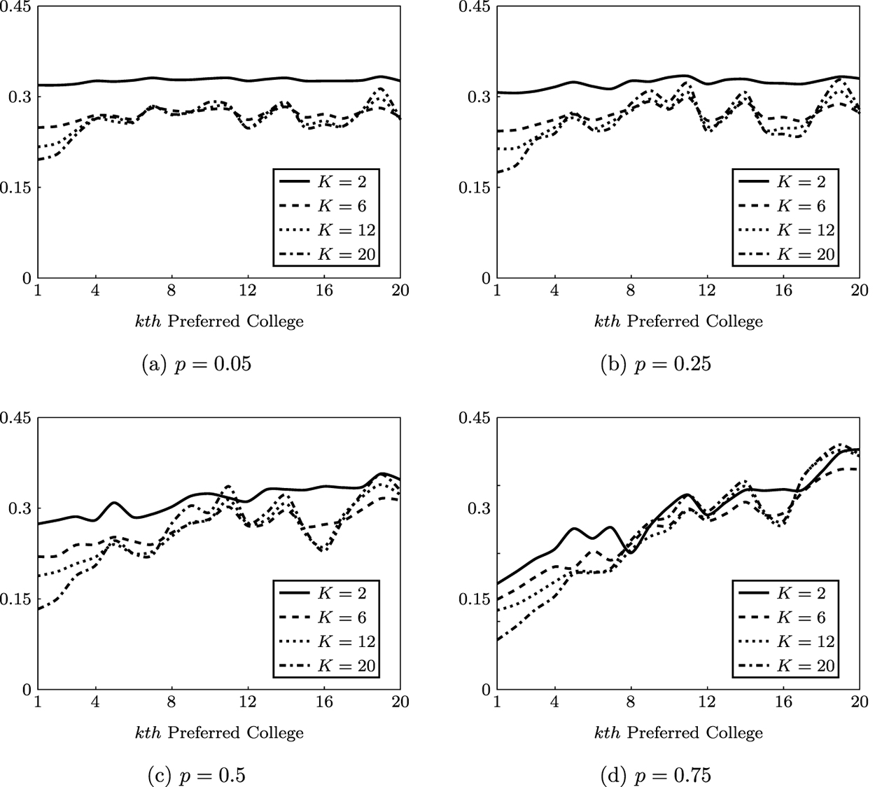
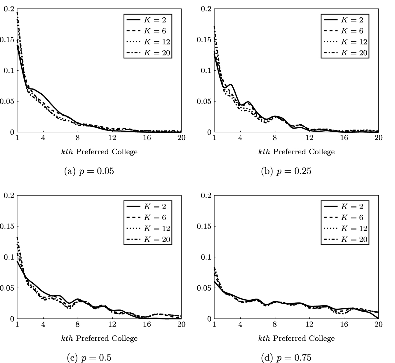
Ex-post probabilities of assignment for all ranked choices. The figure shows the average ex-post probability of assignment for each kth-preferred college. Fixing ρ = 1, panels (Figure 7a)–(Figure 7d) vary the probability of drawing the pivotal type p. The panels shows the ex-post probability for different risk-aversion levels.

Figure 8:

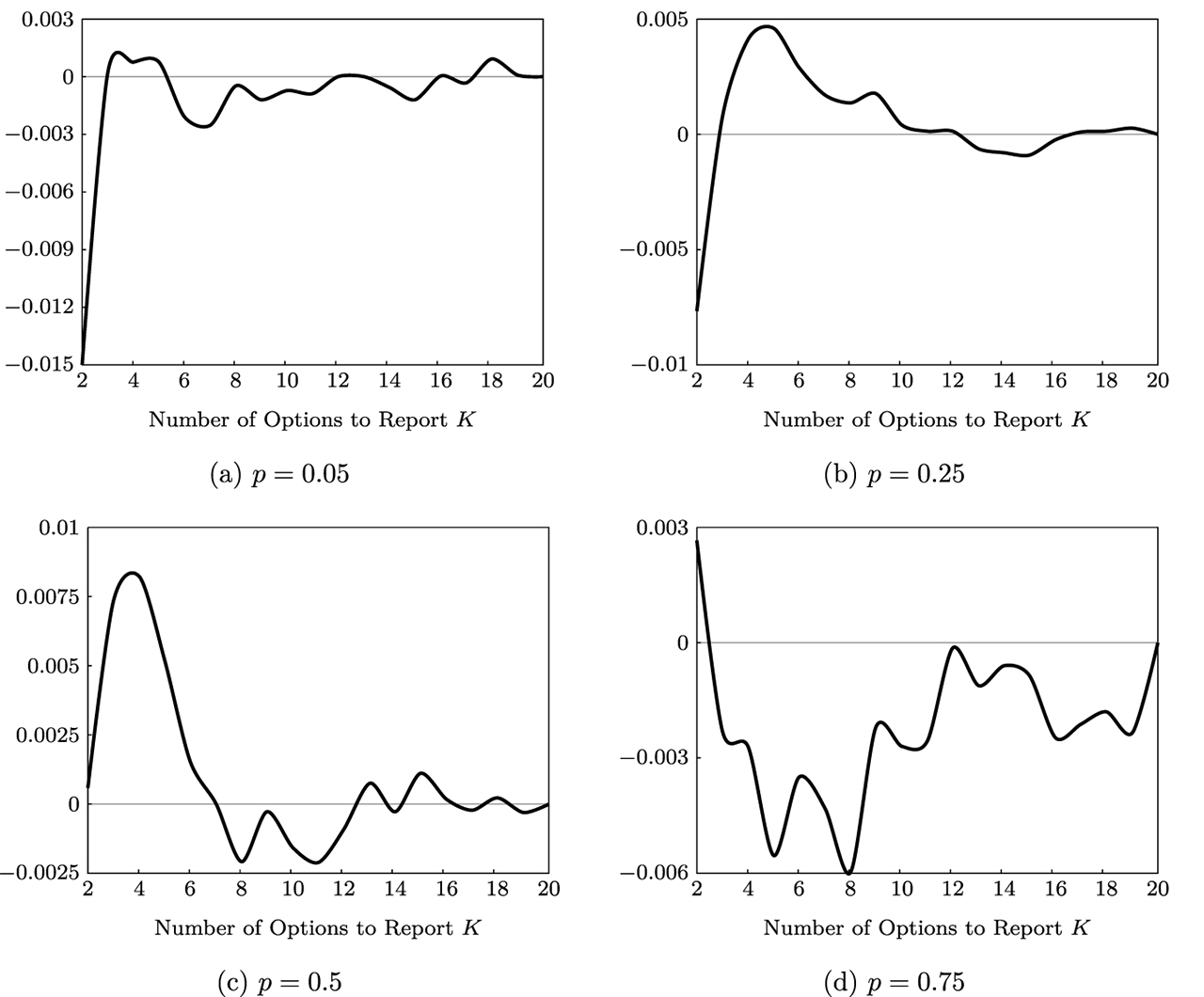
Relative Aggregate Welfare. The panels shows the average aggregate welfare relative to K = 20 for different probabilities of the pivotal profile.

References

Abdulkadiroğlu, A., Y.-K. Che, and Y. Yasuda. 2011. “Resolving Conflicting Preferences in School Choice: The “Boston” Mechanism Reconsidered.” American Economic Review 101 (1): 399–410.10.1257/aer.101.1.399Search in Google Scholar

Abdulkadiroğlu, A., Y.-K. Che, and Y. Yasuda. 2015. “Expanding “Choice” in School Choice.” American Economic Journal: Microeconomics 7 (1): 1–42.10.1257/mic.20120027Search in Google Scholar

Abdulkadiroğlu, A., P. A. Pathak, and A. E. Roth. 2009. “Strategy-Proofness Versus Efficiency in Matching with Indifferences: Redesigning the NYC High School Match.” American Economic Review 99 (5): 1954–78.10.1257/aer.99.5.1954Search in Google Scholar

Abdulkadiroğlu, A., and T. Sönmez. 2003. “School Choice : A Mechanism Design Approach.” American Economic Reivew 93 (3): 729–47.10.1257/000282803322157061Search in Google Scholar

Agarwal, N., and P. Somaini. 2018. “Demand Analysis Using Strategic Reports: An Application to a School Choice Mechanism.” Econometrica 86 (2): 391–444.10.3386/w20775Search in Google Scholar

Azevedo, E. M., and E. Budish. 2018. “Strategy-Proofness in the Large.” The Review of Economic Studies 86 (1): 81–116.10.3386/w23771Search in Google Scholar

Balinski, M., and T. Sönmez. 1999. “A Tale of Two Mechanisms: Student Placement.” Journal of Economic Theory 84 (1): 73–94.10.1006/jeth.1998.2469Search in Google Scholar

Bogomolnaia, A., and H. Moulin. 2001. “A New Solution to the Random Assignment Problem.” Journal of Economic Theory 100 (2): 295–328.10.1006/jeth.2000.2710Search in Google Scholar

Braun, S., N. Dwenger, and D. Kubler. 2010. “Telling the Truth May not Pay Off: An Empirical Study of Centralized University Admissions in Germany.” B.E. Journal of Economic Analysis and Policy 10 (1): 113–22.10.2202/1935-1682.2294Search in Google Scholar

Calsamiglia, C., G. Haeringer, and F. Klijn. 2010. “Constrained School Choice: An Experimental Study.” American Economic Review 100 (4): 1860–74.10.1257/aer.100.4.1860Search in Google Scholar

Chade, H., and L. Smith. 2006. “Simultaneous Search.” Econometrica 74 (5): 1293–307.10.1111/j.1468-0262.2006.00705.xSearch in Google Scholar

Dubins, L. E., and D. A. Freedman. 1981. “Machiavelli and the Gale-Shapley Algorithm.” The American Mathematical Monthly 88 (7): 485–94.10.1080/00029890.1981.11995301Search in Google Scholar

Erdil, A., and H. Ergin. 2008. “What’s the Matter with Tie-Breaking? Improving Efficiency in School Choice.” American Economic Review 98 (3): 669–89.10.1257/aer.98.3.669Search in Google Scholar

Ergin, H. 2002. “Efficient Resource Allocation on the Basis of Priorities.” Econometrica 70 (6): 2489–97.10.1111/1468-0262.00383Search in Google Scholar

Featherstone, C. R., and M. Niederle. 2016. “Boston Versus Deferred Acceptance in an Interim Setting: An Experimental Investigation.” Games and Economic Behavior 100: 353–75.10.1016/j.geb.2016.10.005Search in Google Scholar

Fernández, M., and L. Yariv. 2018 Centralized Matching with Incomplete Information.Search in Google Scholar

Gale, D., and L. S. Shapley. 1962. “College Admissions and the Stability of Marriage.” The American Mathematical Monthly 69 (1): 9–15.10.21236/AD0251958Search in Google Scholar

Haeringer, G., and F. Klijn. 2009. “Constrained School Choice.” Journal of Economic Theory 144 (5): 1921–47.10.1016/j.jet.2009.05.002Search in Google Scholar

Kesten, O. 2006. “On Two Competing Mechanisms for Priority Based Allocation Problems.” Journal of Economic Theory 127 (1): 155–71.10.1016/j.jet.2004.11.001Search in Google Scholar

Kojima, F., and P. Pathak. 2009. “Incentives and Stability in Large Two-Sided Matching Markets.” The American Economic Review 99 (3): 608–27.10.1257/aer.99.3.608Search in Google Scholar

Pais, J., F. Klijn, and M. Vorsatz. 2013. “Preference Intensities and Risk Aversion in School Choice: A Laboratory Experiment.” Experimental Economics 16 (1): 1–22.10.1007/s10683-012-9329-5Search in Google Scholar

Roth, A. E. 1982. “The Economics of Matching: Stability and Incentives.” Mathematics of Operations Research 7 (4): 617–28.10.1287/moor.7.4.617Search in Google Scholar

Roth, A. E. 2002. “The Economist as an Engineer: Game Theory, Experimentation, and Computation as Tools for Design Economics.” Econometrica 70 (4): 1341–78.10.1111/1468-0262.00335Search in Google Scholar

Shapley, L. S., and H. Scarf. 1974. “On Cores and Indivisibility.” Journal of Mathematical Economics 1 (1): 23–37.10.1016/0304-4068(74)90033-0Search in Google Scholar

Troyan, P. 2012. “Comparing School Choice Mechanisms by Interim and Ex-Ante Welfare.” Games and Economic Behavior 75 (2): 936–47.10.1016/j.geb.2012.01.007Search in Google Scholar

Westkamp, A. 2013. “An Analysis of the German University Admission System.” Economic Theory 53 (3): 561–89.10.1007/s00199-012-0704-4Search in Google Scholar

Published Online: 2020-02-19

You are currently not able to access this content.

Articles in the same Issue

https://doi.org/10.1515/bejte-2019-0002

Keywords for this article

college assignment; conditional-alloation effect; consideration effect; constrained choice; private preferences; risk aversion