Collateral Constraints, Wage Rigidity, and Jobless Recoveries
-
Tobias Föll


Abstract
The Great Recession has drawn attention to the importance of macro-financial linkages. In this paper I explore the joint role of imperfections in labor and financial markets for the cyclical adjustment of the labor market. I show that jobless recoveries emerge when, upon exiting a recession, firms are faced with deteriorating credit conditions. On the financial side, collateral requirements affect the cost of borrowing for firms. On the employment side, hiring frictions and wage rigidity increase the need for credit, making the binding collateral constraint more relevant. In a general equilibrium business cycle model with search and matching frictions, I illustrate that tightening credit conditions calibrated from data negatively affect employment adjustments during recovery periods. Wage rigidity substantially amplifies this mechanism, generating empirically plausible fluctuations in employment and output.
1 Introduction
During the 2008 financial crisis, the unemployment rate in the U.S. doubled from 5.0 to 10.0% within only 18 months. While output had fully recovered less than two years after the end of the recession, the unemployment rate took three times as long to reach its pre-crisis level. The marked increase in the unemployment rate was preceded by deteriorating credit conditions and an increase in collateral requirements (cf. Jermann and Quadrini 2012; Garín 2015). As collateral constraints directly affect firms’ hiring decisions, recessions caused by financial frictions might have particularly large adverse effects on the labor market. Motivated by this, I aim to determine the role of disturbances in the financial sector for the U.S. recessions in 1990–1991, 2001, and 2007–2009 and the subsequent jobless recoveries. Following the definition used in, among others, Calvo, Coricelli, and Ottonello (2014), I classify recoveries as jobless if the unemployment rate is above its pre-crisis level by the time output has fully recovered.[1]
Figure 1 depicts the joblessness of the recovery following the Great Recession. After the end of the Great Recession in June 2009 it took slightly less than two years for output to fully recover. At the point of output recovery the unemployment rate had only recovered by about 15% and was still about four percentage points above its pre-crisis level.

Jobless recovery during the Great Recession.
The unemployment rate is the quarterly average of the seasonally adjusted monthly unemployment series constructed by the BLS from the Current Population Survey (CPS). Output is the seasonally adjusted quarterly real GDP from the Bureau of Economic Analysis. For both series the value in 2007Q4 is normalized to 100.
In order to determine the role of financial frictions for jobless recoveries, I add a financial market friction to the standard DSGE model with search and matching frictions, whereby firms need to provide capital as collateral in order to take on loans. Labor and capital are treated asymmetrical, with capital serving a dual role as production factor and as collateral. These elements generate diverging output and employment dynamics during recovery periods and contribute to the emergence of jobless recoveries.
The key interaction in the model arises from the need for funding: due to a cash flow mismatch, firms are required to finance their working capital requirements, including vacancy posting costs, by taking on loans. The presence of financial frictions makes hiring more costly for constrained firms, as they have to cut investment or dividend payouts to finance their wage bill. This implies that the degree to which firms are affected by wage rigidity also varies with credit tightness.
The model is calibrated to U.S. data and simulated using technology and credit shocks, where credit shocks are meant to capture variation in credit conditions. I compare the model dynamics to business cycle statistics for the U.S. between 1964 and 2004. The simulated model with only two shocks can account for nearly 50% of the variation in unemployment, roughly 80% of the fluctuations in vacancies, about 65% of the variation in labor market tightness, and over 90% of the fluctuations in the job-finding rate.
I find that after a negative technology or credit shock, the initial increase in the unemployment rate is stronger and steeper because wage rigidity keeps firms’ borrowing needs high. Financial frictions are responsible for flatter decreases in the unemployment rate: following an increase in productivity, firms prioritize investment into capital as this increases their collateralizable assets. Thus, the initial increase in vacancies and hiring during a recovery period is lower compared to models with perfect credit markets.
The interaction of financial frictions and wage rigidity generates asymmetric unemployment dynamics. I illustrate that the combined effect of these frictions on unemployment dynamics is larger than the sum of the separate effects of financial frictions or wage rigidity. This allows for an amplification of shocks in the model that is close to what is found in the data. In contrast to the results obtained in similar models without financial frictions, even a small and empirically plausible amount of wage rigidity is sufficient to generate highly volatile labor market variables once collateral constraints are taken into account.
Despite the asymmetry in the unemployment rate generated by the combination of a collateral constraint and wage rigidity, recoveries in the model are not jobless unless there is a concomitant erosion of credit conditions. The reason is that credit conditions directly affect the marginal value of an additional worker and thereby the number of hires and the unemployment rate. When credit conditions deteriorate while total factor productivity recovers, unemployment remains above its pre-crisis level. Since capital can be used as production factor and as collateral, the capital stock and output are almost entirely driven by total factor productivity and not by credit conditions. Consequently, recovering total factor productivity, combined with worsening credit conditions, causes jobless recoveries.
This mechanism is consistent with empirical evidence. Analyzing credit conditions during recessions and subsequent recovery periods in the U.S. between 1964 and 2010, I find that prior to 1990 credit conditions started to improve immediately after the end of recessions. During the recent jobless recoveries, credit conditions deteriorated for several quarters after the end of the recessions and the unemployment rate only began to recover once credit conditions had stabilized.
My analysis suggests that low credit availability matters for the occurrence of jobless recoveries after recent recessions. This has important policy implications. Policies aimed at reducing transitional unemployment through reemployment services, such as the $47 billion dollar spent i.a. on job training in the American Recovery and Reinvestment Act of 2009, might not be as effective as hoped: in a model with perfect credit markets, increasing the matching efficiency on the labor market reduces the unemployment rate by twice as much compared to a model with financial frictions. Thus, alternative policies could be aimed at reducing uncertainty on the credit market in order to facilitate job creation.
The remainder of the paper is organized as follows. Previous research is discussed in the next section. The model outline is presented in Section 3. In Section 4 the quantitative analysis is described in detail. Jobless recoveries are discussed in Section 5. To conclude, the results are summarized in Section 6.
2 Related Literature
This paper adds to the literature trying to understand the role of financial conditions for macroeconomic dynamcis (cf. Miao and Wang 2018; Perri and Quadrini 2018; Petrosky-Nadeau and Wasmer 2015; Schwartzman 2012). First steps in this direction have been taken by Kiyotaki and Moore (1997). Wasmer and Weil (2004) introduce search frictions into the credit market and find that the presence of financial frictions increases macroeconomic volatility. Jermann and Quadrini (2012) estimate financial shocks and show that they contribute siginificantly to the dynamics of real and financial variables. Favilukis, Lin, and Zhao (2020) illustrate the importance of labor markets for understanding credit markets, arguing that precommitted labor payments increase the default risk on other committed payments. Drechsel (2021) focuses on the macroeconomic effects of earnings-based borrowing constraints and thus on the connection between a firm’s current earnings and its access to credit. While all of these approaches provide interesting insights, I choose to follow Garín (2015) who introduces financial frictions in the style of Kiyotaki and Moore (1997) into a search and matching framework, which provides a direct link between collateral requirements and asset prices and allows for changes in credit availability to directly affect firms’ job creation decision.
Closely related to this work are Schoefer (2016) and Moiseeva (2018) who both study the interaction of financial frictions and wage rigidity in a search and matching framework. However, neither of the models presented in these papers is able to generate jobless recoveries. In Moiseeva (2018), since the financial costs of hiring are high in recessions, firms delay hiring until the recession has passed. While this mechanism amplifies fluctuations in labor market variables, the rapid increase in hiring after a recession stands in sharp contrast to the observation of jobless recoveries. Schoefer (2016) explores a channel similar to the one presented here, through which wage rigidity and financial frictions influence a firm’s job creation decision. Since labor is the only production factor in Schoefer (2016), any asymmetry in unemployment mechanically spills over to output dynamics as long as technology shocks are symmetric. Thus, after a recession, employment will have fully recovered at the point of output recovery.
Finally, this paper adds to the literature that studies the role of financial conditions for jobless recoveries.[2] Schott (2013) distinguishes between incumbent firms and startups and argues that low credit availibility for young firms is responsible for the lack of job creation. Wesselbaum (2019) emphasizes the role of financial frictions under match efficiency shocks. Calvo, Coricelli, and Ottonello (2014) make the case that jobless recoveries are caused by the interaction of financial frictions and wage rigidity. To illustrate their empirical findings, they analyze a stylized competitive model of the labor market with an ad-hoc borrowing constraint. In their model, productivity growth leads to jobless recoveries when the borrowing constraint binds and wages are rigid. I demonstrate that these conditions are not sufficient for the emergence of jobless recoveries in a general equilibrium framework with an endogenous borrowing constraint. Additionally, since the labor market in Calvo, Coricelli, and Ottonello (2014) is assumed to be competitive, wage rigidity is essential in generating jobless recoveries. My findings suggest that while wage rigidity amplifies the extent of jobless recoveries, it is not a prerequisite for their occurrence.
3 A Model with Financial Frictions and Wage Rigidity
In this section, I introduce wage rigidity into a simple version of the model presented in Garín (2015).[3] The model economy is populated by two types of agents: workers and capitalists. Capitalists own the firms, which produce a homogenous good y t using labor n t and physical capital k t . All dividends d t are transferred to the capitalists. Households consist of a continuum of workers, are assumed to perfectly share all risks, and have access to a one-period riskless bond a t that is issued by capitalists and used for consumption smoothing.
The labor market is subject to search frictions in the sense of Mortensen and Pissarides (1994): hiring workers entails vacancy posting costs that are paid by the firms. Wages are determined by standard Nash bargaining over the entire surplus of a worker-firm match.
Due to a cash-flow mismatch, firms need to raise funds via intra-period loans l t in order to finance their working capital requirements. Since contract enforcement is costly, these loans require collateral.
3.1 The Labor Market
The number of matches on the labor market is determined by
At the beginning of each period, a fraction x of all existing worker-firm matches is exogenously separated. Newly separated workers immediately begin searching for a new job and have the same job-finding rate as all other unemployed workers. Employment evolves according to
and at the end of each period
workers remain unemployed. Since search is costless from the household perspective, all non-employed workers search for a job.
Posting a vacancy entails costs of
3.2 Households
The setup allows for the existence of a representative household, consisting of a continuum of workers of measure one. The household aims at maximizing lifetime utility by allocating consumption optimally across all members:
where c t is consumption, β h is the discount factor of the household, φ is the disutility from work, and n t is the share of workers that is employed at time t.[5] The household’s flow of funds constraint is given by
Employed workers earn wages w t and unemployed workers receive benefits s. The benefits are financed through a lump-sum tax T t = (1 − n t )s. The one-period riskless bond a t pays an interest rate of R t and is used for consumption smoothing.[6]
The representative household chooses consumption and the number of bonds in order to maximize the expected discounted lifetime utility over consumption and leisure. Since it takes the job-finding rate as given, employment evolution from the household perspective can be described by
The complete household maximization problem is given in Appendix A. Combining the first order conditions with respect to consumption and bonds results in the standard Euler equation
Intuitively, the household invests into bonds until the marginal utility of today’s consumption is equal to the discounted marginal utility of consuming tomorrow, weighted by the rental rate R t .
3.3 Financial Markets
Due to a cash-flow mismatch firms need to raise funds via intra-period loans l t in order to finance their working capital requirements.[7] Wage payments, dividend payouts, investment, current debt, and vacancy posting costs all accrue before the realization of revenues. Since contract enforcement is costly, firms are subject to a collateral requirement. Following a default, financial intermediaries cannot seize production. Only the installed capital stock can be recovered and sold at η t q k,t k t , where q k,t is the marginal Tobin’s Q and η t captures uncertainty regarding the tightness of the credit market. As is standard in the literature, financial intermediaries are assumed to have no bargaining power in the debt renegotiation and they do not value the stock of workers in the firm (cf. Garín 2015; Perri and Quadrini 2018). η t is interpreted as an exogenous collateral shock following the stochastic process
with
The derivation of the enforcement constraint follows the derivation in Garín (2015). Referring to the respective optimization problem, the value of a firm can be written as
where the vector
With the possibility of default before the loan is due and after production is realized, the value of not defaulting is
In the case of default, firms and lenders renegotiate. If an agreement is reached, firms pay lenders a fraction ν t of the continuation value. Therefore, the value of a successful renegotiation is
where firms continue to produce, get another loan l t , but have to pay a part of the continuation value to the lenders. As production cannot be seized by lenders in the case of default, the value of an unsuccessful renegotiation for the firm is simply ν f,u = l t . Consequently, the net value of an agreement is given by
From the perspective of a lender, the value of a successful renegotiation is
In the case that no agreement is reached, lenders cannot seize production. As they do not value the stock of workers in the firm, the value of an unsuccessful renegotiation is
from the lender’s point of view. This results in the net value of an agreement for the lender of
The joint surplus of renegotiating is the sum of the net values of the firm and the lender. Since financial intermediaries have no bargaining power in the renegotiation of debt, the firm gets the value
in case of a default. This value is equal to its liquidity plus the joint surplus of renegotiating the debt. In order to rule out defaults, the value of not defaulting for the firm has to be at least as large as the value of defaulting. Using this inequality and rearranging terms results in the enforcement constraint
which constrains a firm’s ability to borrow below the value of the fraction of the physical capital stock that lenders can recuperate after default.
3.4 Firms
Capitalists are risk-averse and derive utility from the consumption of dividend payouts. They can only access the financial market through the firm and are assumed to be more impatient than households, i.e. β h > β c , where β c is the discount factor of the firm.[8] Thus, capitalists’ expected lifetime utility is a function of dividends,
As firms are owned by capitalists, the objective of a firm is to maximize the expected future stream of discounted dividends. Firms own the capital stock k
t
and use it together with labor n
t
to produce a homogenous good with
subject to the budget constraint
the law of motion for the capital stock
the law of motion for employment,
and the borrowing constraint
where the loan l t is replaced by the working capital requirements. Denoting the multipliers on the budget constraint, the law of motion for the capital stock, the law of motion for employment, and the borrowing constraint with μ c,t , μ k,t , μ e,t , and μ b,t , respectively, and taking derivatives results in the following first order conditions:
where q k is the ratio of the Lagrange multipliers μ k,t and μ c,t . As is standard in the literature, q k,t represents the value of the installed capital relative to its replacement costs.
The marginal value of an additional worker for the firm
where
Proposition 1
The effect of wage rigidity on the hiring decision is larger for a financially constrained firm.
Proof
The elasticity of the marginal value of an additional worker with respect to the wage rate is given by
The absolute value of this elasticity increases with μ b,t . As the marginal value of relaxing the borrowing constraint increases proportionally with collateral requirements, the elasticity of the marginal value of an additional worker with respect to changes in the wage increases with collateral requirements, too. □
This implies that the marginal benefit of hiring an additional worker reacts more strongly to changes in the wage rate compared to standard search and matching models. Consequently, even a small amount of wage rigidity has large effects on labor market variables in my model.
3.5 Wage Bargaining and Wage Rigidity
As is standard in most of the search and matching literature, wages are determined as the solution of a generalized Nash bargaining problem. The production function exhibits constant returns to scale, which greatly simplifies the bargaining problem, as models with diminishing returns are subject to the critique by Stole and Zwiebel (1996). Moreover, I assume that firms first hire workers, subsequently bargain about wages, and only then choose the capital stock, which further simplifies the bargaining problem (cf. Cahuc and Wasmer 2001). The wage equation is thus given by[9]
Since the model economy is subject to two kinds of shocks, wage rigidity in the style of Blanchard and Galí (2010) or Michaillat (2012) is not feasible. Instead, as in Hall (2005) and Krause and Lubik (2007), wage rigidity is introduced through a backward-looking wage norm that limits the adjustment capability of wages
where
Proposition 2
Assume that the wage schedule is given by Eq. (15). Wages are privately efficient if the wage schedule satisfies
Proof
See Appendix E. □
This proposition implies that no worker-firm match generating a positive bilateral surplus is separated because of wage rigidity as long as the actual wage remains within the postulated bounds. Thus, the wage schedule in Eq. (15) is not subject to the Barro (1977) critique that bargaining workers and firms should be able to exploit all possible bilateral gains in long-term worker-firm relationships with reoccuring wage renegotiations. Due to constant returns in production, the model is also not affected by the critique of Brügemann (2017) concerning wage rigidity in search and matching models with diminishing returns.
3.6 Equilibrium
With the model completely described, I define the equilibrium.
Definition 1
A recursive equilibrium is defined as a set of (i) firm’s policy functions d(ω c ; Ω), b(ω c ; Ω), k(ω c ; Ω), n(ω c ; Ω), i(ω c ; Ω), and v(ω c ; Ω); (ii) household’s policy functions c(ω h ; Ω), n(ω h ; Ω), and a(ω h ; Ω); (iii) a lump sum tax T(Ω), (iv) prices w(Ω) and R(Ω); and (v) a law of motion for the aggregate states, Ω′ = Ψ(Ω), such that: (i) the firm’s policies satisfy the firm’s first order conditions (Eqs. (8)–(12)) and the job creation condition (Eq. (13)); (ii) household’s policy function satisfies the household’s first order condition (Eq. (2)), (iii) the wage is determined by Eq. (15); (iv) R(Ω) clears the market for riskless assets such that a(Ω) = b(Ω); (v) labor demand equals labor supply; (vi) the law of motion Ψ(Ω) is consistent with individual decisions and with the stochastic processes for z and η, and (vii) the government has a balanced budget such that s(1 − n) = T.
4 Quantitative Analysis
In this section, I calibrate all parameters discussed above to match different aspects of quarterly U.S. data for the time period between the first quarter of 1964 and the fourth quarter of 2004.[10] I use the calibrated model to simulate time series of all variables. The model performance is evaluated along several dimensions, most importantly with respect to unemployment dynamics.
4.1 Calibration
Table 1 lists the exact parameter values as well as the source that encourages the specific choice. The discount factors are set to β h = 0.996 and β c = 0.983. The assumption β h > β c implies that the annual interest rate will be lower than the annual return on equity. The specific choices match an annual interest rate of 1.6% and an annual return on equity of 7%.
Calibration of the model parameters.
| Symbol | Interpretation | Value | Source/target |
|---|---|---|---|
| β h | Household’s discount factor | 0.996 | Annual interest rate of 1.6% |
| β c | Firms’ discount factor | 0.983 | Annual return on equity of 7% |
| x | Separation rate | 0.1 | Shimer (2005) |
|
|
Recruiting costs | 0.18 | Michaillat (2012) |
| ν | Matching efficiency | 0.651 | Job-finding rate of 0.8 |
| γ | Unemployment-elasticity of matching | 0.5 | Petrongolo and Pissarides (2001) |
| s | Unemployment benefits | 0.4 | Replacement rate of 0.2 |
| φ | Disutility of labor | 0.85 | Unemployment rate of 11% |
| τ | Renegotiation probability | 0.25 | Taylor (1999); Gottschalk (2005) |
| ξ | Investment adjustment cost | 0.050 | Lower end of literature values |
|
|
Steady state credit market tightness | 0.2923 | Debt-to-output ratio of 1.59 |
| σ | Agents relative risk aversion | 2 | Standard in the literature |
| φ | Worker’s bargaining power | 0.4 | Midpoint of literature values |
| α | Marginal returns to labor | 0.66 | Labor share of 0.66 |
| ρ z | Autocorrelation of technology shocks | 0.9524 | Solow residual |
| σ z | Standard deviation of technology shocks | 0.0080 | Solow residual |
| ρ η | Autocorrelation of credit shocks | 0.9340 | Midpoint of literature values |
| σ η | Standard deviation of credit shocks | 0.0116 | Volatility debt-to-output ratio |
| δ | Capital depreciation rate | 0.025 | Jermann and Quadrini (2012) |
Next, I calibrate the labor market variables. For the separation rate, I choose a conventional value of 0.1 (cf. Shimer 2005). Regarding vacancy posting costs, there is a relatively wide range of admissable values in the literature. Silva and Toledo (2009) estimate recruitment costs equal to 3.6% of a worker’s monthly wage. Using microdata by Barron, Berger, and Black (1997), Michaillat (2012) estimates the costs of posting a vacancy at 9.8% of a worker’s steady state wage. Vacancy costs calibrated to match the latter value imply steady state vacancy posting costs of 0.28% of the total wage bill and 0.17% of GDP in Michaillat (2012). I calibrate κ/2 to 0.18, which is slightly more than 9% of a worker’s steady state wage. Given this value, steady state vacancy posting costs account for 0.31% of the total wage bill and 0.2 % of GDP.
The efficiency of the matching function is chosen to match a quarterly job-finding rate of 0.8 and the elasticity of the matching function with respect to unemployment to match empirical evidence from Petrongolo and Pissarides (2001). Unemployment benefits are set to 0.4. This value implies a steady state replacement rate of about 0.2, which is at the lower end of the values found in the literature and implies a ratio of unemployment benefits to consumption of 0.23. The parameter φ, governing the disutility of labor, is set to match a steady state unemployment rate of 11%.[11]
Next, I calibrate the parameter governing wage rigidity based on the interpretation of the wage schedule arising from a staggered Nash bargaining setting as in Gertler and Trigari (2009). Equation (15) is the equivalent of the wage equation in Gertler and Trigari (2009) under financial frictions if neither firms nor workers take into account that they might not be able to renegotiate wages in the subsequent periods. With this calibration strategy, τ can be interpreted as representing an upper bound on wage rigidity. Taylor (1999) argues that medium sized and large firms typically readjust wages anually. Additional evidence is provided by Gottschalk (2005), who finds that wage adjustments are most common one year after the last change. Thus, I set τ to 0.25, implying an average renegotiation frequency of once per year.
Since investment adjustment costs can potentially generate asymmetric unemployment dynamics, they are cautiously set to ξ = 0.05, a value at the very low end of the values found in the literature.[12]
Using the dataset constructed by Jermann and Quadrini (2012), the parameters for the persistence and standard deviation of the technology shocks are calculated using an approach similar to the one used to calculate Solow residuals. The parameters for the mean, persistence, and standard deviation of the credit shocks are calibrated to capture important aspects of the data. The mean of the credit shock process,
4.2 Simulated Moments
I compare the simulated moments of the model to business cycle statistics for U.S. data. For the vacancy series I take data from Michaillat (2012), who merged the Job Openings and Labor Turnover Survey (JOLTS) for 2001–2004 with the Conference board help-wanted advertising index for 1964–2001. Unemployment data is taken from the Bureau of Labor Statistics (BLS) and labor market tightness is calculated as the ratio of vacancies to unemployment. For each of these series I take the quarterly average. The real wage estimates are average hourly earnings in the nonfarm business sector constructed by the BLS Current Employment Statistics. Output is quarterly real output from the BLS Major Sector Productivity and Costs program. In order to isolate business cylce fluctuations, I use a Hodrick-Prescott filter with smoothing parameter 100.000 as recommended in Shimer (2005).[13]
I simulate 264 quarters of data corresponding to the empirical sample size of 1964:I to 2004:IV.[14] The data is detrended using the same HP filter. The simulation is repeated 500 times and each repetition provides an estimate of the means of the simulated data. While the technology and credit shock processes are calibrated to match the empirical data, all other simulated moments are outcomes of the mechanics of the model. All simulations are performed using a second-order perturbation method. Since I am interested in asymmetric unemployment dynamics, a first order approximation is obviously not feasible. As the results remain virtually unchanged when using third- or fourth-order approximations, a second-order approximation seems to capture most of the relevant dynamics.
Table 2 displays the second order moments for key labor market variables both for U.S. data and for the simulated model. The model performs well along most dimensions that a model without financial frictions and without wage rigidity fails to capture.[15] While the standard deviation of unemployment is still too low compared to U.S. data, it is about four times the standard deviation of output. In addition, the model accounts for roughly 65% of the volatility of labor market tightness, 80% of the volatility in vacancies, and over 90% of the fluctuations in the job-finding rate. Robustness exercises in the form of business cycle statistics for a model with financial frictions but without wage rigidity and for a model with wage rigidity but without financial frictions are provided in Appendix F. These simulations confirm that the interaction between wage rigidity and financial frictions, and not only the sum of the separate effects, plays an important role in matching business cycle statistics and in explaining unemployment dynamics.
Data versus model simulation.
| Quarterly U.S. data, 1964–2004 | ||||||
|---|---|---|---|---|---|---|
| u | v | θ | w | y | z | |
| Standard deviation | 0.166 | 0.186 | 0.339 | 0.021 | 0.030 | 0.020 |
| Autocorrelation | 0.918 | 0.946 | 0.934 | 0.949 | 0.902 | 0.890 |
| Correlation | 1 | −0.888 | −0.968 | −0.114 | −0.820 | −0.514 |
| 1 | 0.975 | 0.162 | 0.762 | 0.488 | ||
| 1 | 0.140 | 0.810 | 0.514 | |||
| 1 | 0.499 | 0.639 | ||||
| 1 | 0.883 | |||||
| 1 | ||||||
| Model with financial frictions and wage rigidity τ= 0.25 | ||||||
| u | v | θ | w | y | z | |
| Standard deviation | 0.077 | 0.153 | 0.214 | 0.012 | 0.021 | 0.016 |
| Autocorrelation | 0.827 | 0.416 | 0.570 | 0.960 | 0.859 | 0.842 |
| Correlation | 1 | −0.791 | −0.888 | −0.523 | −0.844 | −0.756 |
| 1 | 0.974 | 0.250 | 0.635 | 0.591 | ||
| 1 | 0.358 | 0.736 | 0.679 | |||
| 1 | 0.836 | 0.800 | ||||
| 1 | 0.975 | |||||
| 1 | ||||||
-
All data are seasonally adjusted. The sample period is 1964:I – 2004:IV. The unemployment rate u is the quarterly average of the monthly series constructed by the BLS from the CPS. Vacancies are taken from Michaillat (2012) and constructed as detailed in the text. Labor market tightness θ is the ratio of vacancies to unemployment. For the real wage I use quarterly average hourly earnings in the nonfarm business sector constructed by the BLS Current Employment Statistics program and deflated by the quarterly average of the monthly Consumer Price Index for all urban households, constructed by the BLS; y is the quarterly real output in the nonfarm business sector constructed by the BLS Major Sector Productivity and Costs dataset; ln(z) is constructed as a residual. Following Haefke, Sonntag, and van Rens (2013), fluctuations in the capital stock are ignored. Simulation results are obtained by simulating the model with stochastic technology and credit tightness with a second-order perturbation method. All variables are log deviations from an HP trend with smoothing parameter 105.
Shocks are amplified considerably in the model: a 1% decrease in productivity increases unemployment by 3.6%, decreases vacancies by 5.7%, and decreases labor market tightness by 9.1%.[16] In the data, a 1% decrease in productivity increases unemployment by 4.2%, decreases vacancies by 4.5%, and decreases labor market tightness by 8.6%. The response of vacancies and labor market tightness is a bit higher in the model than in the data, which might be due to a lower elasticity of wages with respect to changes in technology. Haefke et al. (2013) find an elasticity of about 0.7, while the presented business cycle statistics for the U.S. suggest a value of 0.65. The simulated elasticity is a bit lower with a value of 0.6.
Comparing the elasticity of unemployment to technology in this model with the elasticity in a model with perfect credit markets, I find that the effect of wage rigidity is six times larger when firms are constrained in their ability to borrow. Additionally, the effect of financial frictions on the elasticity of unemployment to technology is more than twice as large under wage rigidity compared to a model with flexible wages. As they reinforce each other, the combined effect of wage rigidity and financial frictions is two times larger than the sum of the two separate effects.
Next, I turn to the asymmetric behavior of the cyclical component of the unemployment rate documented and analyzed in, for example, McKay and Reis (2008), Barnichon (2010), and Atolia, Gibson, and Marquis (2018). Following Sichel (1993), I measure asymmetry in unemployment dynamics with the skewness coefficient.[17] For U.S. data in the time period between 1964 and 2004, the skewness of the unemployment rate is 0.72 in levels and 1.30 in changes.[18] These values suggest that the unemployment rate is characterized by short periods of sharp increases and long periods of flat decreases.
Figure 2 illustrates the asymmetry of the unemployment rate in the model based on the impulse response functions. The absolute value of the deviation of the unemployment rate from its steady state following a positive one standard deviation shock to technology is subtracted from the deviation of the unemployment rate from its steady state following a negative shock to technology of the same size. A value larger than zero implies that the deviation of the unemployment rate is larger after a negative shock. The asymmetry is most pronounced for the model with financial frictions and wage rigidity. In contrast, the impulse response functions for output are almost completely symmetric.
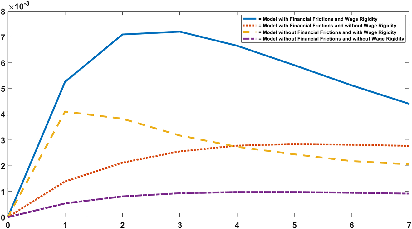
Asymmetric impulse response functions: unemployment.
This figure plots the difference between the deviation of the unemployment rate from its steady state following a negative one standard deviation shock to technology and the absolute value of the deviation of the unemployment rate from its steady state following a positive one standard deviation shock to technology.
Table 3 displays the skewness of the simulated unemployment rate in levels and in changes for different amounts of wage rigidity.[19] A standard search and matching model with symmetric shocks is unable to match these observations despite the inherent asymmetry resulting from costly vacancy posting, which is frequently emphasized in the literature (cf. Petrosky-Nadeau, Zhang, and Kuehn 2018; Hairault, Langot, and Osotimehin 2010). The simulated unemployment series in a benchmark model without financial frictions and without wage rigidity displays a skewness of 0.12 in levels and 0.02 in changes, explaining only about 17 and 2% of the respective skewness in the data.[20] In the model with financial frictions and wage rigidity, the skewness of the simulated unemployment series is 0.49 in levels and 0.27 in changes. About 75% of the skewness in levels and nearly 25% of the skewness in changes in the data can be explained by combining both frictions in a search and matching framework.[21]
Skewness of the simulated unemployment rate.
| τ = 1 | τ = 0.5 | τ = 0.25 | ||
|---|---|---|---|---|
| With financial frictions | Levels | 0.33 | 0.38 | 0.49 |
| Changes | 0.22 | 0.24 | 0.27 | |
| Without financial frictions | Levels | 0.12 | 0.13 | 0.18 |
| Changes | 0.02 | 0.03 | 0.05 |
-
The amount of wage rigidity τ implies an average renegotiation frequency of three months, six months, and twelve months, respectively.
As with the elasticity of unemployment to technology shocks, financial frictions and wage rigidity reinforce their respective effects. The combined effect of wage rigidity and financial frictions on the skewness in levels is 48% larger than the sum of the two separate effects. For the skewness in changes the combined effect is 9% larger.[22]
5 Jobless Recoveries
In this section, I first illustrate the ability of the model to generate jobless recoveries. Simulating the model for the time period between 1964 and 2010, I confirm that it generates jobless recoveries following the recessions in 1999–1991, 2001, and 2007–2009, whereas prior to 1990 employment is predicted to have fully recovered at the point of output recovery after recessions. Subsequently, the model performance is evaluated against the data, comparing the predictions on unemployment dynamics, employment growth, investment, and the capital-labor-ratio to their empirical counterparts.
Having established that the model is able to generate jobless recoveries, I take a detailed look at the underlying mechanism. Analyzing the impulse response functions to technology and credit shocks, I illustrate that despite the considerable skewness in the simulated unemployment rate, neither a pure technology shock nor a pure credit shock is followed by a jobless recovery in the model. I argue that jobless recoveries emerge when credit conditions continue to erode during recovery periods while total factor productivity already recovers. Finally, I provide empirical evidence for the proposed mechanism.
5.1 Simulated Recoveries
In a first step, I demonstrate that a DSGE model with frictional labor and financial markets is able to generate jobless recoveries. Technology and credit shock series are calibrated to match the behavior of output during the Great Recession. The resulting series for output and unemployment are depicted in Figure 3. Negative shocks to credit tightness and to technology cause a recession in which output decreases by 4% during the first four quarters. Technology recovers but credit conditions continue to deteriorate. Firms invest into capital and output fully recovers after six to seven quarters. At the point of output recovery the unemployment rate has only recovered by around 31% relative to its peak (compared to a recovery by 15% after the Great Recession) and is two percentage points above its pre-crisis level (compared to four percentage points after the Great Recession).

Simulated Great Recession.
The jobless recovery is generated using series of technology and credit shocks in the simulated model with financial frictions and wage rigidity. The shock series are calibrated to match the behavior of output during the Great Recession. The pre-recession levels of unemployment and output are normalized to 100.
The model does not rely on wage rigidity to generate jobless recoveries. This stands in sharp contrast to the results obtained by Calvo, Coricelli, and Ottonello (2014) using a competitive labor market model. Nonetheless, the joblessness of the recovery period is more pronounced under wage rigidity. Without wage rigidity, the unemployment rate would have recovered by about 45% at the point of output recovery.
Next, I consider the ability of the model to account for jobless recoveries given technology and credit shocks estimated from the data. To that end I use the dataset provided by Jermann and Quadrini (2012) to estimate credit and technology shock series for the time period between 1964 and 2010.[23] The estimated shock series are depicted in Figure 4.
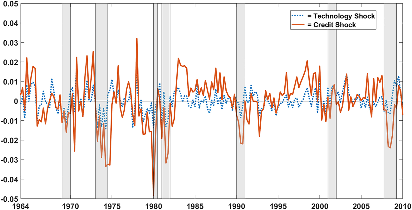
Estimated technology and credit shock series, 1964–2010.
The technology shock and credit shock series are estimated from the dataset to Jermann and Quadrini (2012). Periods classified as recessions by the National Bureau of Economic Research (NBER) are highlighted in gray.
Figure 5 plots the simulated series for unemployment and output. In line with U.S. data, the model only predicts jobless recoveries following the recessions after 1990. At the point of output recovery after the recessions in 1990–1991, 2001, and 2007–2009, the simulated unemployment rate has only recovered by 62, 38, and 68%, respectively, compared to its peak.[24] In all simulated recoveries following recessions prior to 1990, the unemployment rate has fully recovered at the point of output recovery. Overall, the simulated model is able to account for 64% of the variation in the unemployment rate over the considered time period.
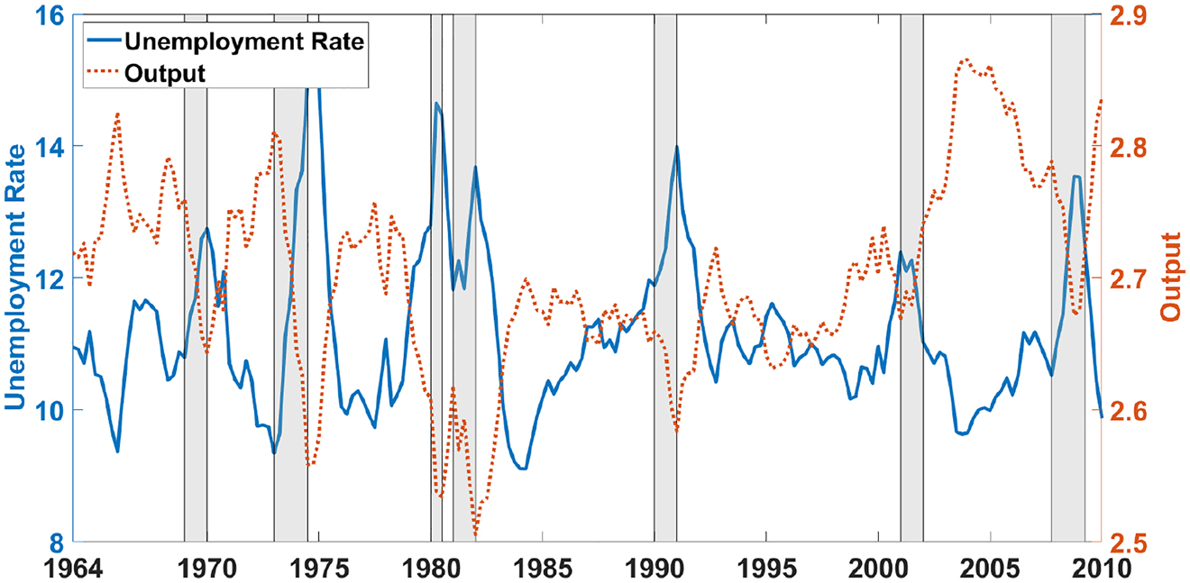
Simulated unemployment and output, 1964–2010.
Output and unemployment are simulated using technology shock and credit shock series estimated from the dataset to Jermann and Quadrini (2012). Periods classified as recessions by the NBER are highlighted in gray.
Turning to the initial capital deepening commonly observed in the U.S. during recessionary periods, the model predicts an increase of 1.6% in the capital-labor-ratio during the recession in 1990–1991, 2.6% during the recession in 2001, and 2.6% during the recession in 2007–2009, explaining between 66 and 90% of the increase observed in the data.[25] Moreover, both in the model and in the data, the capital-labor-ratio peaks slightly after the end of the recessions.
Table 4 displays the development of output and employment in the model and in the data for the three U.S. recessions after 1990. In line with the data, the model predicts employment to be below its peak value two years after the peak for all three recessions. Comparing the recent recessions with recessions prior to 1990, lower employment after two years is a unique feature of jobless recoveries.[26]
5.2 Impulse Response Functions
In this section, I present the impulse response functions of several variables to a negative one standard deviation shock to total factor productivity and a negative one standard deviation shock to credit tightness. The scale represents log deviations from steady state.
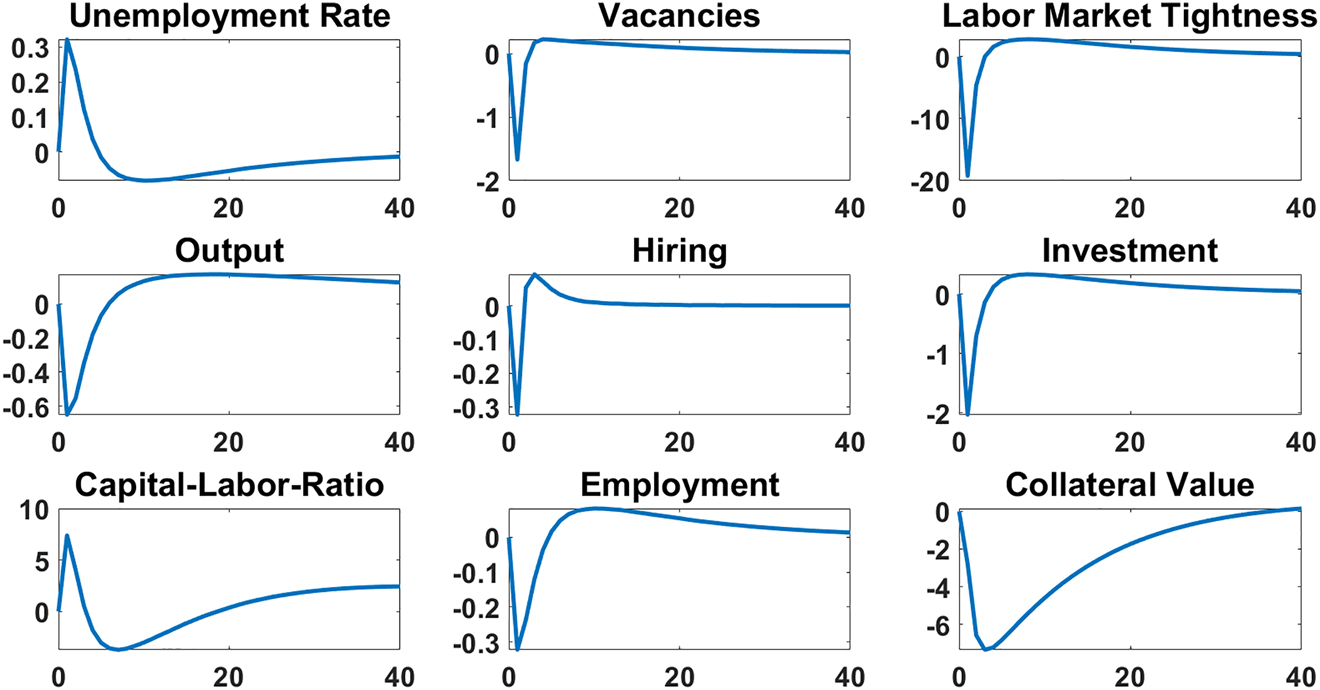
The impulse response functions for a negative shock to technology depicted in Figure 6 comply with the literature. Following a negative shock, firms decrease hiring with vacancies dropping by nearly 9% on impact. The unemployment rate increases, leading to an even larger decrease in labor market tightness. The marginal value and the collateral value of the capital stock drop, which triggers the decrease in investment. As the initial decrease in hiring is larger compared to the initial increase in investment, the capital-labor-ratio increases on impact and only drops below its steady state value after several periods. The hump-shaped response of both the unemployment rate and investment is generated by the respective adjustment costs.[27]
Impulse response functions: negative technology shock.
The scale represents percentage deviations from the steady state. The size of the technology shock is one standard deviation.
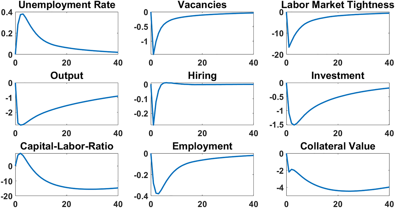
Figure 7 depicts the response of the model to a negative one standard deviation shock to credit market tightness. Firms are immediately able to borrow less against their collateral and respond by sharply cutting hiring and investment on impact. This lowers the future capital stock and further tightens the credit constraint. The drop in vacancies, however, is not persistent. Lower expenditures reduce working capital requirements and the capital-labor-ratio increases, which relaxes the borrowing constraint and allows firms to increase investment and vacancies again in the following periods. Still, the initial drop in vacancies is large enough to generate a persistent increase in the unemployment rate. After dropping on impact, hiring increases above its steady state value long before output has recovered.[28]
Impulse response functions: negative credit shock.
The scale represents percentage deviations from the steady state. The size of the credit shock is one standard deviation.
Note that neither technology nor credit shocks are able to generate dynamics in the unemployment rate that are more persistent than output dynamics. Therefore, and in contrast to the results obtained by Calvo, Coricelli, and Ottonello (2014) in a competitive model of the labor market, neither a simple shock to credit tightness nor a simple shock to total factor productivity is able to induce a jobless recovery in a DSGE model with labor market frictions, rigid wages, and an endogenous borrowing constraint.
5.3 Mechanism
In my model, regardless of whether the recession is caused by a technology or by a credit shock, output and unemployment behave very similarly as long as only one shock drives the economy. Jobless recoveries emerge when credit conditions continue to erode while total factor productivity recovers. They are jobless because worsening credit conditions are an important driver of unemployment dynamics and keep unemployment high, but play only a minor role for fluctuations in output. In the variance decomposition exercise in Table 5, over 30% of the fluctuations in unemployment are caused by credit shocks, while virtually all of the fluctuations in output are due to productivity shocks.[29]
Changes in employment and output: model versus data.
| Output | Employment | ||||
|---|---|---|---|---|---|
| Data | Model | Data | Model | ||
| 1990–1991 recession | 1 year | −0.7% | −2.8% | −1.1% | −1.6% |
| 2 years | 2.3% | 0.3% | −0.5% | −0.5% | |
| 2001 recession | 1 year | 1.5% | −1.1% | −1.2% | −1.7% |
| 2 years | 3.3% | 2.1% | −0.3% | −0.3% | |
| 2007–2009 recession | 1 year | −3.3% | −2.4% | −1.7% | −2.0% |
| 2 years | −3.8% | −0.7% | −5.5% | −0.8% | |
-
The growth rates are calculated by comparing peak output and employment at the start of the recession (or within one quarter) with output and employment one and two years later. Employment is total nonfarm payroll employment from the BLS Current Employment Statistics. Output is the seasonally adjusted quarterly real GDP from the Bureau of Economic Analysis.
Figure 8, which depicts the effect of a positive one standard deviation shock to technology on the ratio of investment to hiring, illustrates this mechanism. With financial frictions, a positive technology shock tightens the credit constraint as it increases working capital requirements. Rather than to increase hiring, firms invest into the asset used as collateral, as this puts less strain on the borrowing constraint. The increase in employment is delayed and the decrease in unemployment is flatter compared to standard search and matching models. Relative to the increase in hiring, the increase in investment is most pronounced in the model with financial frictions and wage rigidity, reflecting the preference of firms to invest into the asset used as collateral after a positive technology shock.
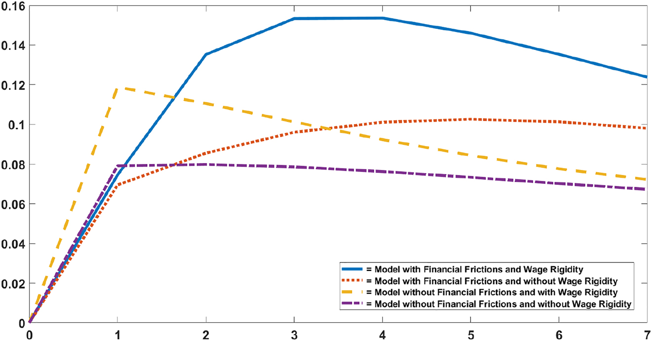
Impulse response functions: investment/hiring.
This figure plots the impulse response function of the ratio of investment to hiring (i/m) following a one standard deviation positive technology shock.
The mechanism is also evident in the first order conditions of the firm. Credit conditions directly affect the marginal value of an additional worker. A tightening of future credit conditions increases μ b,t+1, the Lagrange multiplier on the borrowing constraint, and thus the marginal value of relaxing this constraint. The increase in credit tightness reduces the marginal value of an additional worker by
Now consider the effect of the same increase in credit tightness on the marginal value of an additional unit of capital
As for the marginal value of an additional worker, the increase in credit tightness reduces the marginal value of the capital stock in the production process. However, capital can also be used as collateral, the value of which increases with credit tightness. Thus, the effect of credit shocks on unemployment is larger than the effect of credit shocks on capital and output.[30] When total factor productivity recovers after a recession, firms increase their capital stock which in turn increases production. If this recovery is accompanied by tightening credit conditions, the marginal value of an additional worker stays low and at the point of output recovery the unemployment rate will be above its pre-crisis level.
5.4 Empirical Evidence
Evidence for deteriorating credit conditions during jobless recoveries can be found in the dataset provided by Jermann and Quadrini (2012) as well as in the Senior Loan Officer Opinion Survey on Bank Lending Practices from FRED.
Table 6, which displays the average size of credit shocks following the end of a recession estimated from the dataset provided by Jermann and Quadrini (2012), is used to gauge the development of credit conditions following recessionary periods in the U.S. A negative value implies a tightening of credit conditions. Prior to the two jobless recoveries in 1990–1991 and in 2001, credit conditions remained virtually constant immediately after the end of a recession.[31] Following the end of the recessions in 1990–1991 and in 2001, credit conditions continued to worsen with the credit shocks amounting to −1.4 and −0.82 times a standard deviation of the estimated credit shock series on average.
Variance decomposition.
| y | u | v | θ | w | |
|---|---|---|---|---|---|
| TFP shocks | 97.04 | 68.41 | 52.19 | 58.38 | 98.53 |
| Credit shocks | 2.96 | 31.59 | 47.81 | 41.62 | 1.47 |
-
The variance decomposition is used to assess the relative importance of technology and credit shocks for generating volatility in the simulated model.
Credit shocks during recoveries.
| Average Credit Shock | |
|---|---|
| Recessions prior to 1990 | −0.00248 |
| 1990–1991 recession | −1.3968 |
| 2001 recession | −0.8237 |
-
I define the average credit shock after a recessionary period as the average size of the credit shocks in the four quarters following the end of a recession normalized by the standard deviation of the credit shock series. The credit shock series for the time period between 1964 and 2010 is estimated from the dataset provided by Jermann and Quadrini (2012). The recession in 1980 is left out of the sample as the recovery period is overlaid by the start of the recession in 1981. The Great Recession is left out as the dataset only covers the time period up to the first quarter of 2010.
A tightening of credit conditions during the recent recoveries, including the recovery after the Great Recession, is also reported in the Senior Loan Officer Opinion Survey on Bank Lending Practices from FRED depicted in Figure 9.[32] Credit market tightness is calculated as the fraction of surveyed banks reporting to tighten credit standards minus the fraction of banks reporting to lower their standards. A positive value therefore implies a tightening of credit conditions.
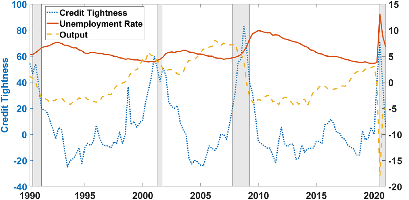
Unemployment rate, output, and credit market tightness, 1990–2021.
The unemployment rate is the quarterly average of the seasonally adjusted monthly unemployment series constructed by the BLS from the CPS. Credit market tightness is measured as the Net Percentage of Domestic Respondents Tightening Standards for Commercial and Industrial Loans for Medium and Large Firms obtained from the Senior Loan Officer Opinion Survey on Bank Lending Practices from FRED. Output is the quarterly, detrended real gross domestic product in billions of chained 2012 dollars from FRED. Periods classified as recessions by the NBER are highlighted in gray.
Two observations are striking. First, following the end of all three recessions, credit conditions continued to deteriorate – for several months after the recessions in 1990–1991 and in 2007–2009, and for nearly two years after the recession in 2001. Second, following the end of the recessions, the unemployment rate only began to decrease after credit conditions had stabilized.
Further evidence for the mechanism is provided in Figure 10, which depicts gross real investment and the unemployment rate. After the recessions in 1990–1991 and 2001, investment had recovered by 26.7 and 47.7%, respectively, before unemployment even began to recover. Two years after the Great Recession, at the point of output recovery, investment had recovered by over 78% while unemployment had only recovered by 15%.
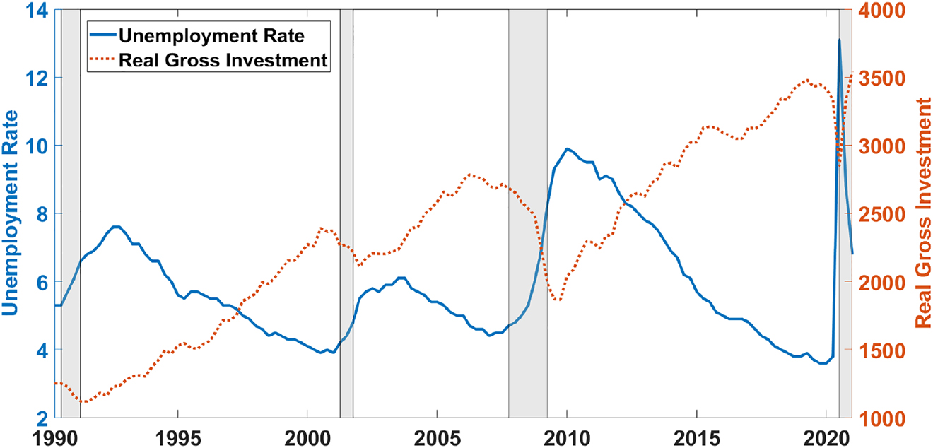
Unemployment rate and real gross investment, 1990–2021.
The unemployment rate is the quarterly average of the seasonally adjusted monthly unemployment series constructed by the BLS from the CPS. Real gross investment is measured as the seasonally adjusted FRED Real Gross Private Domestic Investment series measured in billions of chained 2012 dollars. Periods classified as recessions by the NBER are highlighted in gray.
Finally, Figure 11 displays the unemployment rate for different industries between 2000 and 2021. In line with the model predictions, industries that exhibit large working capital requirements and rely heavily on collateralized borrowing, like the construction and manufacturing industries, have experienced a lot steeper increases in the unemployment rates during the Great Recession compared to, for example, the telecommunications industry or other service industries.[33] Moreover, Jaimovich and Siu (2020) point out that the manufacturing and construction industries have been exceptionally affected by the recessions in 1990–1991, 2001, and 2007–2009 and that subsequent recoveries have been jobless in both industries, whereas in prior recovery periods manufacturing and construction employment displayed strong cyclical rebounds. This suggests a high relevance of the proposed mechanism for those industries that heavily rely on collateralized borrowing at the very least.[34]
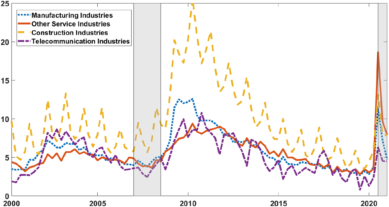
Unemployment rate by industries, 2000–2021.
The unemployment rates by industries are taken from the Labor Force Statistics from the CPS provided by the BLS. The data series is available from 2000 onward. The other services sector consists of the repair and maintenance industry, the personal and laundry services industry, service industries labeled as religious, grantmaking, civic, professional, and similar organizations, as well as private household services. Periods classified as recessions by the NBER are highlighted in gray.
6 Conclusion
Incorporating financial frictions and wage rigidity considerably improves the performance of the standard search and matching model. Besides increasing the volatility of key labor market variables, the interaction of the two frictions facilitates the replication of important aspects of unemployment dynamics.
The simulated model with only technology and credit shocks can account for nearly 50% of the variation in unemployment, roughly 80% of the fluctuations in vacancies, about 65% of the variation in labor market tightness, and over 90% of the fluctuations observed in the job-finding rate. I find that wage rigidity is responsible for the steeper increase in the unemployment rate after negative shocks, whereas credit constraints ensure that decreases after positive shocks are flatter. Jobless recoveries are induced by eroding credit conditions during recovery periods.
While the explored mechanism provides an easy way to add important dynamics to search and matching models, it might also be able to reconcile models with endogenous separations with the highly negative correlation between unemployment and vacancies, i.e. the Beveridge curve. In models with endogenous separations, the unemployment pool increases disproportionately after a negative technology shock due to the large inflow of separated workers. This decreases the labor market tightness and makes hiring in recessions cheap. Most models with endogenous separations therefore entail on-the-job search in order to reconcile the model with the data. In a model with endogenous separations and financial frictions, unemployment will also increase disproportionately after a negative credit shock. However, the incentive to post vacancies is reduced by a tightening of the borrowing constraint. It is an interesting task for further research to explore whether this mechanism is strong enough to generate a highly negative vacancy-unemployment correlation.
Appendix A: Household’s Maximization Problem
Having defined the state vectors in Section 3, the household maximization problem can be written as
subject to
where the vector
Appendix B: Wage Bargaining
In order to derive the wage schedule, I first define the value functions
and
where λ
t
is the Lagrange multiplier on the household’s budget constraint. The marginal value of a match,
where
With both value functions defined, the wage that solves the bargaining problem can be expressed as
where ϕ is the bargaining power of the worker. Taking the first derivative results in the standard first order condition
that can be rewritten as
In the next step I define the total surplus of the match
Using
In the last step I replace
Appendix C: Role of Investment Adjustment Costs
In this section I deviate from the conservative choice of investment adjustment costs in the main text. A parameter value at the lower end of the range found in the literature was chosen for the quantitative analysis because higher investment adjustment costs increase the incentive for firms to keep fluctuations in investment low. This increases the volatility of labor market variables and strengthens the asymmetric behavior of unemployment.
To asses the theoretical ability of the model mechanisms to generate positive skewness in the unemployment rate, the investment adjustment costs are increased by a factor 10 to the value used in an early version of Perri and Quadrini (2018), ξ = 0.5. Under the new parametrization, the skewness of the unemployment rate increases to 0.86 in levels (0.72 in the data) and 0.61 in changes (1.30 in the data). All of the skewness in levels and nearly 50% of the skewness in changes is explained by financial frictions in conjunction with wage rigidity under high investment adjustment costs.
Even though investment adjustment costs can generate skewed unemployment dynamics in my model, I confirm that they are not the main driving force behind the results in this paper. Setting the adjustment costs to zero reduces the skewness of the simulated unemployment rate by less than 5%. This implies that a value of ξ = 0.05 is already small enough as not to blur the emphasized mechanism.
Appendix D: Benchmark Model
The model described in this section exhibits perfect credit markets and flexible wages. It acts as a benchmark in the quantitative analysis in order to gauge the performance of the complete model with financial frictions and wage rigidity. The benchmark model is based on the appendix to Garín (2015). The labor market and the household sector are unchanged by the introduction of financial frictions. Therefore, the first two subsections from Section 3 hold for this model as well.
D.1 Firms
Under the same assumptions as in Section 3, the maximization problem of the firm can be expressed as
subject to the budget constraint
the law of motion for the capital stock
and the law of motion for employment
Denoting the multipliers on the budget constraint, the law of motion for the capital stock, and the law of motion for employment, with μ c,t , μ k,t , and μ e,t respectively, and taking derivatives results in the following first order conditions:
Under these specifications, the marginal value of an additional worker for the firm is given by
The first term is the net return of an additional worker for the firm. The second term is the discounted benefit of having an additional worker in the next period. Combining the marginal value with Eq. (D.5) yields the job creation condition
Again, the firm hires additional workers until the marginal costs of hiring equal the marginal benefits. In contrast to the model in Section 3, the job creation condition does not depend on financial conditions.
D.2 Wage Bargaining
Since the financial frictions introduced in Section 3 only affect the firm side, the marginal value of the match for the household is the same as in the model with financial frictions. With both value functions defined, the wage that solves the bargaining problem can be expressed as
where ϕ is a parameter that governs the bargaining power of the worker and the firm. Taking the first derivative results in the standard first order condition
that can be rewritten as
As a next step I define the total surplus of the match
where I use that λ
t
= u′(c
t
). Next, I use Eq. (B.1),
In the last step I replace
D.3 Equilibrium
With the model completely described, I define the equilibrium.
Definition 2
A recursive equilibrium is defined as a set of (i) firm’s policy functions d(ω c ; Ω), k(ω c ; Ω), n(ω c ; Ω), i(ω c ; Ω), and v(ω c ; Ω); (ii) household’s policy functions c(ω h ; Ω) and n(ω h ; Ω); (iii) a lump-sum tax T(Ω), (iv) prices w(Ω) and R(Ω); and (v) a law of motion for the aggregate states, Ω′ = Ψ(Ω), such that: (i) firm’s policies satisfy the firm’s first order conditions (Eqs. (D.4)–(D.8)) and the job creation condition (Eq. (D.10)); (ii) household’s policy function satisfies the household’s first order condition (Eq. (2)), (iii) the wage is determined by Eq. (D.11); (iv) labor demand equals labor supply; (v) the law of motion Ψ(Ω) is consistent with individual decisions and with the stochastic process for technology z, and (vi) the government has a balanced budget such that s(1 − n) = T.
D.4 Simulation Results
The model without financial frictions and without wage rigidity is calibrated to match the same steady state values as the complete model. Simulation results are given in Table D.7 and are strikingly close to the results obtained by Shimer (2005) in the simulation of a model with only labor productivity shocks. While the model performance is good along several important dimensions, it is unable to match the high volatility of the key labor market variables unemployment, vacancies, and labor market tightness. The volatiliy of vacancies and labor market tightness is even lower than in Shimer (2005), as the presence of capital and bonds in the benchmark model gives firms more possibilities to adjust to technology shocks.
Simulated moments – flexible wages and perfect credit markets.
| u | v | θ | w | y | z | |
|---|---|---|---|---|---|---|
| Standard deviation | 0.009 | 0.014 | 0.023 | 0.014 | 0.016 | 0.015 |
| Autocorrelation | 0.940 | 0.792 | 0.865 | 0.839 | 0.845 | 0.830 |
| Correlation | 1 | −0.891 | −0.958 | −0.941 | −0.947 | −0.933 |
| 1 | 0.983 | 0.970 | 0.974 | 0.994 | ||
| 1 | 0.985 | 0.991 | 0.996 | |||
| 1 | 0.999 | 0.990 | ||||
| 1 | 0.992 | |||||
| 1 |
-
Results from simulating the model with stochastic technology with a second-order perturbation method. All variables are log deviations from an HP trend with smoothing parameter 105.
Appendix E: Private Efficiency of Wages
Proof
The proof draws from the proof of private efficiency in the online appendix to Michaillat (2012). The goal of the proof is to derive necessary and sufficient conditions under which positive bilateral gains from the match ensure that neither firms nor workers have any incentive to separate. In a first step, I illustrate that as long as wages lie above the threshold that ensures higher utility than the value of unemployment, workers do not quit. In a second step, I derive the conditions under which firms hire additional workers, freeze hiring, and lay off workers. In the third and final step, I argue that as hiring freezes in a symmetric equilibrium drive the hiring costs to zero, each individual firm has an incentive to be the only firm hiring. Thus, hiring freezes are ruled out and the condition for avoiding layoffs is identical to the upper bound that ensures private efficiency of wages.
The first part of the proof is relatively straightforward. For the household side private efficiency implies that the marginal value of an additional matched worker has to be positive:
This equation can be rearranged to give
The household has no incentive to have the last worker separated from the match if the wage plus the continuation value of the match is larger than unemployment benefits plus the utility value of leisure. Since I focus only on symmetric equilibria, all firms pay equal wages and no worker has an incentive to switch firms.
For the second part of the proof, let the marginal revenue of an additional worker be defined by
which is the highest marginal product the firm can receive in a given period without laying off workers. Assume that there exist marginal costs
if
if
if
subject to
and
where
and
where L
t+1 is the value function of the firm as seen from period t + 1.
where
Using the value function, it follows that
and
Next, note that in a symmetric environment hiring freezes occur with a probability of zero. As the environment is symmetric, if one firm decides to freeze hiring all firms will do so. However, when all firms freeze hiring, θ is equal to zero, as there are no vacancies. This implies
Using this equation, a necessary and sufficient condition to avoid layoffs is
which is equal to the equation in Proposition 2.
Appendix F: Further Business Cycle Statistics
In this section, I evaluate the business cycle statistics for the benchmark model with wage rigidity and for the model with financial frictions but without wage rigidity. This robustness exercise emphasizes the importance of the interaction between wage rigidity and financial frictions, not only for explaining unemployment dynamics, but also for explaining business cycle statistics. I strengthen this point by showing that neither the benchmark model with wage rigidity nor the model with financial frictions and without wage rigidity is able to generate volatility in labor market variables comparable to the data. The results are displayed in Table F.8.
Further business cycle statistics.
| Financial frictions and τ = 0 | ||||||
|---|---|---|---|---|---|---|
| u | v | θ | w | y | z | |
| Standard deviation | 0.049 | 0.106 | 0.145 | 0.013 | 0.018 | 0.016 |
| Autocorrelation | 0.785 | 0.297 | 0.458 | 0.848 | 0.867 | 0.842 |
| Correlation | 1 | −0.780 | −0.884 | −0.496 | −0.637 | −0.445 |
| 1 | 0.977 | 0.370 | 0.469 | 0.350 | ||
| 1 | 0.433 | 0.548 | 0.401 | |||
| 1 | 0.981 | 0.972 | ||||
| 1 | 0.959 | |||||
| 1 | ||||||
| Benchmark model and τ = 0.25 | ||||||
| u | v | θ | w | y | z | |
| Standard deviation | 0.012 | 0.024 | 0.037 | 0.012 | 0.017 | 0.015 |
| Autocorrelation | 0.888 | 0.610 | 0.726 | 0.949 | 0.849 | 0.830 |
| Correlation | 1 | −0.837 | −0.929 | −0.798 | −0.947 | −0.967 |
| 1 | 0.979 | 0.499 | 0.817 | 0.865 | ||
| 1 | 0.630 | 0.899 | 0.938 | |||
| 1 | 0.904 | 0.857 | ||||
| 1 | 0.993 | |||||
| 1 | ||||||
-
Results from simulating the model with stochastic technology and credit tightness with a second-order perturbation method. All variables are log deviations from an HP trend with smoothing parameter 105.
Without wage rigidity, the volatility of the key labor market variables drops sharply. The volatility of unemployment decreases by 37%, the volatility of vacancies by 31%, and the volatility of labor market tightness by 32%. The response of unemployment, vacancies and labor market tightness to a 1% percent decrease in productivity is lower: unemployment increases by 1.4%, vacancies decrease by 2.3%, and labor market tightness decreases by 3.6%.
For the benchmark model, the introduction of wage rigidity increases the volatility of unemployment by 45%, the volatility of vacancies by 71%, and the volatility of labor market tightness by 61%. Despite the large relative increases, the absolute values remain small. Even with larger wage rigidity than in the model with financial frictions, the benchmark model does not generate enough amplification to match the empirical volatility of the key labor market variables or the amplification of shocks in the data.
References
Atolia, M., J. Gibson, and M. Marquis. 2018. “Asymmetry and the Amplitude of Business Cycle Fluctuations: A Quantitative Investigation of the Role of Financial Frictions.” Macroeconomic Dynamics 22 (2): 279–306. https://doi.org/10.1017/s1365100516000171.Search in Google Scholar
Barnichon, R. 2010. “The Lumpy Job Separation Rate: Reconciling Search Models with the Ins and Outs of Unemployment.” Working Paper.10.17016/FEDS.2009.24Search in Google Scholar
Barro, R. J. 1977. “Long-term Contracting, Sticky Prices, and Monetary Policy.” Journal of Monetary Economics 3 (3): 305–16. https://doi.org/10.1016/0304-3932(77)90024-1.Search in Google Scholar
Barron, J. M., M. C. Berger, and D. A. Black. 1997. “Employer Search, Training and Vacancy Duration.” Economic Inquiry 35 (1): 167–92. https://doi.org/10.1111/j.1465-7295.1997.tb01902.x.Search in Google Scholar
Berger, D. 2012. “Countercyclical Restructuring and Jobless Recoveries.” Working Paper.Search in Google Scholar
Blanchard, O., and P. Diamond. 1990. “The Cyclical Behavior of the Gross Flows of U.S. Workers.” Brookings Papers on Economic Activity 1990 (21): 85–156. https://doi.org/10.2307/2534505.Search in Google Scholar
Blanchard, O., and J. Galí. 2010. “Labor Markets and Monetary Policy: A New Keynesian Model with Unemployment.” American Economic Journal: Macroeconomics 2 (2): 1–30. https://doi.org/10.1257/mac.2.2.1.Search in Google Scholar
Brügemann, B. A. 2017. “Privately Efficient Wage Rigidity under Diminishing Returns.” Working Paper.Search in Google Scholar
Cahuc, P., and E. Wasmer. 2001. “Does Intrafirm Bargaining Matter in the Large Firms Matching Model.” Macroeconomic Dynamics 5 (5): 742–7. https://doi.org/10.1017/s1365100501031042.Search in Google Scholar
Calvo, G. A. 2015. “The Liquidity Approach to Bubbles, Crises, Jobless Recoveries, and Involuntary Unemployment.” Journal Economía Chilena 18 (3): 4–27.Search in Google Scholar
Calvo, G. A., Coricelli, F., and Ottonello, P. 2014. “Labor Market, Financial Crises and Inflation: Jobless and Wageless Recoveries.” NBER Working Paper No. 18480.Search in Google Scholar
Chugh, S. K. 2013. “Costly External Finance and Labor Market Dynamics.” Journal of Economic Dynamics and Control 37 (12): 2882–912. https://doi.org/10.1016/j.jedc.2013.08.005.Search in Google Scholar
DeNicco, J. P. 2015. “Employment-at-will Exceptions and Jobless Recovery.” Journal of Macroeconomics 45: 245–57. https://doi.org/10.1016/j.jmacro.2015.05.003.Search in Google Scholar
Drechsel, T. 2021. “Earnings-based Borrowing Constraints and Macroeconomic Fluctuations.” Working Paper.Search in Google Scholar
Elsby, M. W., R. Michaels, and G. Solon. 2009. “The Ins and Outs of Cyclical Unemployment.” American Economic Journal: Macroeconomics 1 (1): 84–110. https://doi.org/10.1257/mac.1.1.84.Search in Google Scholar
Erickson, T., and T. M. Whited. 2012. “Treating Measurement Error in Tobin’s Q.” Review of Financial Studies 25 (4): 1286–329. https://doi.org/10.1093/rfs/hhr120.Search in Google Scholar
Favilukis, J., X. Lin, and X. Zhao. 2020. “The Elephant in the Room: The Impact of Labor Obligations on Credit Markets.” The American Economic Review 110 (6): 1673–712. https://doi.org/10.1257/aer.20170156.Search in Google Scholar
Fujita, S., and G. Ramey. 2006. “The Cyclicality of Job Loss and Hiring.” In Working Papers 06-17. Federal Reserve Bank of Philadelphia.10.21799/frbp.wp.2006.17Search in Google Scholar
Galí, J., F. Smets, and R. Wouters. 2012. “Slow Recoveries: A Structural Interpretation.” Journal of Money, Credit, and Banking 44 (2): 9–30. https://doi.org/10.1111/j.1538-4616.2012.00552.x.Search in Google Scholar
Garín, J. 2015. “Borrowing Constraints, Collateral Fluctuations, and the Labor Market.” Journal of Economic Dynamics and Control 57: 112–30. https://doi.org/10.1016/j.jedc.2015.05.007.Search in Google Scholar
Garín, J., M. J. Pries, and E. R. Sims. 2011. “Reallocation and the Changing Nature of Economic Fluctuations.” Working Paper.Search in Google Scholar
Gertler, M., and A. Trigari. 2009. “Unemployment Fluctuations with Staggered Nash Bargaining.” Journal of Political Economy 117 (1): 38–86. https://doi.org/10.1086/597302.Search in Google Scholar
Gottschalk, P. 2005. “Downward Nominal Wage Flexibility: Real or Measurement Error.” The Review of Economics and Statistics 87 (3): 556–68. https://doi.org/10.1162/0034653054638328.Search in Google Scholar
Groshen, E., and S. Potter. 2003. “Has Structural Change Contributed to a Jobless Recovery?” Current Issues in Economics and Finance - Federal Reserve Bank of New York 9: 1–7.Search in Google Scholar
Haefke, C., M. Sonntag, and T. van Rens. 2013. “Wage Rigidity and Job Creation.” Journal of Monetary Economics 60 (8): 887–99. https://doi.org/10.1016/j.jmoneco.2013.09.003.Search in Google Scholar
Hairault, J., F. Langot, and S. Osotimehin. 2010. “Matching Frictions, Unemployment Dynamics and the Cost of Business Cycles.” Review of Economic Dynamics 13 (4): 759–79. https://doi.org/10.1016/j.red.2010.05.001.Search in Google Scholar
Hall, R. E. 2005. “Employment Fluctuations with Equilibrium Wage Stickiness.” The American Economic Review 95 (1): 50–65. https://doi.org/10.1257/0002828053828482.Search in Google Scholar
Hayashi, F. 1982. “Tobin’s Marginal Q and Average Q: A Neoclassical Interpretation.” Econometrica 50 (1): 213–24. https://doi.org/10.2307/1912538.Search in Google Scholar
Jaimovich, N., and H. E. Siu. 2020. “The Trend Is the Cycle: Job Polarization and Jobless Recoveries.” The Review of Economics and Statistics 102 (1): 129–47. https://doi.org/10.1162/rest_a_00875.Search in Google Scholar
Jermann, U. J., and V. Quadrini. 2012. “Macroeconomic Effects of Financial Shocks.” The American Economic Review 102 (1): 238–71. https://doi.org/10.1257/aer.102.1.238.Search in Google Scholar
Kaas, L., and P. Kircher. 2015. “Efficient Firm Dynamics in a Frictional Labor Market.” The American Economic Review 105 (10): 3030–60. https://doi.org/10.1257/aer.20131702.Search in Google Scholar
Kiyotaki, N., and J. Moore. 1997. “Credit Cycles.” Journal of Political Economy 105 (2): 211–48. https://doi.org/10.1086/262072.Search in Google Scholar
Krause, M. U., and T. Lubik. 2007. “The (Ir)relevance of Real Wage Rigidity in the New Keynesian Model with Search Frictions.” Journal of Monetary Economics 54 (3): 706–27. https://doi.org/10.1016/j.jmoneco.2005.12.001.Search in Google Scholar
Lin, X., C. Wang, N. Wang, and J. Yang. 2018. “Investment, Tobin’s Q, and Interest Rates.” Journal of Financial Economics 130 (3): 620–40. https://doi.org/10.1016/j.jfineco.2017.05.013.Search in Google Scholar
McKay, A., and R. Reis. 2008. “The Brevity and Violence of Contractions and Expansions.” Journal of Monetary Economics 55 (4): 738–51. https://doi.org/10.1016/j.jmoneco.2008.05.009.Search in Google Scholar
Meltzer, A. 2003. “Jobless Recovery.” The Wallstreet Journal, Also available at https://www.wsj.com/articles/SB106453705442294900.Search in Google Scholar
Merz, M., and E. Yashiv. 2007. “Labor and the Market of the Firms.” The American Economic Review 97 (4): 1419–31. https://doi.org/10.1257/aer.97.4.1419.Search in Google Scholar
Miao, J., and P. Wang. 2018. “Asset Bubbles and Credit Constraints.” The American Economic Review 108 (9): 2590–628. https://doi.org/10.1257/aer.20160782.Search in Google Scholar
Michaillat, P. 2012. “Do matching Frictions Explain Unemployment? Not in Bad Times.” The American Economic Review 102 (4): 1721–50. https://doi.org/10.1257/aer.102.4.1721.Search in Google Scholar
Moiseeva, Y. 2018. “The Interaction between Credit and Labour Market Frictions.” Working Paper.Search in Google Scholar
Mortensen, D. T., and C. A. Pissarides. 1994. “Job Creation and Job Destruction in the Theory of Unemployment.” The Review of Economic Studies 61 (3): 397–415. https://doi.org/10.2307/2297896.Search in Google Scholar
Perri, F., and V. Quadrini. 2018. “International Recessions.” The American Economic Review 108 (4-5): 935–84. https://doi.org/10.1257/aer.20140412.Search in Google Scholar
Petrongolo, B., and C. A. Pissarides. 2001. “Looking into a Black Box: A Survey of the Matching Function.” Journal of Economic Literature 39 (2): 390–431. https://doi.org/10.1257/jel.39.2.390.Search in Google Scholar
Petrosky-Nadeau, N. 2014. “Credit, Vacancies and Unemployment Fluctuations.” Review of Economic Dynamics 17: 191–205. https://doi.org/10.1016/j.red.2013.10.001.Search in Google Scholar
Petrosky-Nadeau, N., and E. Wasmer. 2015. “Macroeconomic Dynamics in a Model of Goods, Labor, and Credit Market Frictions.” Journal of Monetary Economics 72: 97–113. https://doi.org/10.1016/j.jmoneco.2015.01.006.Search in Google Scholar
Petrosky-Nadeau, N., L. Zhang, and L.-A. Kuehn. 2018. “Endogenous Disasters.” The American Economic Review 108 (8): 2212–45. https://doi.org/10.1257/aer.20130025.Search in Google Scholar
Schmitt-Grohé, S., and M. Uribe. 2017. “Liquidity Traps and Jobless Recoveries.” American Economic Journal: Macroeconomics 9 (1): 165–204. https://doi.org/10.1257/mac.20150220.Search in Google Scholar
Schoefer, B. 2016. “The Financial Channel of Wage Rigidity.” Working Paper.Search in Google Scholar
Schott, I. 2013. “Startups, Credit, and the Jobless Recovery.” Working Paper.Search in Google Scholar
Schwartzman, F. F. 2012. “When Do Credit Frictions Matter for Business Cycles?” FRB Economic Quarterly 98 (3): 209–30.Search in Google Scholar
Shimer, R. 2005. “The Cyclical Behavior of Equilibrium Unemployment and Vacancies.” The American Economic Review 95 (1): 25–49. https://doi.org/10.1257/0002828053828572.Search in Google Scholar
Shimer, R. 2012. “Wage Rigidities and Jobless Recoveries.” Journal of Monetary Economics 59: 65–77. https://doi.org/10.1016/j.jmoneco.2012.10.024.Search in Google Scholar
Sichel, D. E. 1993. “Business Cycle Asymmetry: A Deeper Look.” Economic Inquiry 31 (2): 224–36. https://doi.org/10.1111/j.1465-7295.1993.tb00879.x.Search in Google Scholar
Silva, J. I., and M. Toledo. 2009. “Labor Turnover Costs and the Cyclical Behavior of Vacancies and Unemployment.” Macroeconomic Dynamics 13 (S1): 76–96. https://doi.org/10.1017/s1365100509080122.Search in Google Scholar
Stock, J. H., and M. W. Watson. 1999. “Forecasting Inflation.” Journal of Monetary Economics 44 (2): 293–335. https://doi.org/10.1016/s0304-3932(99)00027-6.Search in Google Scholar
Stole, L. A., and J. Zwiebel. 1996. “Intra-firm Bargaining under Non-binding Contracts.” The Review of Economic Studies 63 (3): 375–410. https://doi.org/10.2307/2297888.Search in Google Scholar
Tauringana, V., and G. A. Afrifa. 2013. “The Relative Importance of Working Capital Management and its Components to SMEs Profitability.” Journal of Small Business and Enterprise Development 20 (3): 453–69. https://doi.org/10.1108/jsbed-12-2011-0029.Search in Google Scholar
Taylor, J. B. 1999. “Staggered Price and Wage Setting in Macroeconomics.” Handbook of Macroeconomics 1: 1009–50. https://doi.org/10.1016/s1574-0048(99)10023-5.Search in Google Scholar
Waddle, A. 2019. “Globalization and Jobless Recoveries.” Journal of Macroeconomics 62: 103138. https://doi.org/10.1016/j.jmacro.2019.103138.Search in Google Scholar
Wasmer, E., and P. Weil. 2004. “The Macroeconomics of Credit and Labor Market Imperfections.” The American Economic Review 94 (4): 944–63. https://doi.org/10.1257/0002828042002525.Search in Google Scholar
Wesselbaum, D. 2019. “Jobless Recoveries: The Interaction between Financial and Search Frictions.” Journal of Macroeconomics 61: 103126. https://doi.org/10.1016/j.jmacro.2019.103126.Search in Google Scholar
Supplementary Material
The online version of this article offers supplementary material (https://doi.org/10.1515/bejm-2020-0221).
© 2021 Walter de Gruyter GmbH, Berlin/Boston
Articles in the same Issue
- Frontmatter
- Advances
- Uncertainty, Financial Markets, and Monetary Policy over the Last Century
- Collateral Constraints, Wage Rigidity, and Jobless Recoveries
- Revisiting the Link between House Prices and Monetary Policy
- Front-Loading Agricultural Subsidies: Quantifying Public Savings
- Contributions
- Equilibrium Tax Rates under Ex-ante Heterogeneity and Income-dependent Voting
- Financial Reforms and Consumption Smoothing
- The Government in SNA-Compliant DSGE Models
- Accounting for the International Great Depression: Efficiency, Distortions and Factor Utilization during the Interwar Period
- Assessing the Role of Sentiment in the Propagation of Fiscal Stimulus
- Fiscal Decentralization and Fiscal Multiplier in China
- Effect of Feed-In Tariff with Deregulation on Directed Technical Change in the Energy Sector
- Pay-as-You-Go Social Security and Educational Subsidy in an Overlapping Generations Model with Endogenous Fertility and Endogenous Retirement