Predicting Recidivism of Juvenile Offenders
-
David E. Kalist


Abstract
This study uses a large data set to analyze and predict recidivism of juvenile offenders in Pennsylvania. We employ a split-population duration model to determine the effect of covariates on (1) the probability of failure, defined as a second referral to juvenile court, and (2) the time to failure, given that it occurs. A test of the predictive power of our estimates finds a false positive rate of 18.5% and a false negative rate of 20.7%, which compares favorably to the performance of other models in the literature.
1 Introduction
Juvenile crime is a matter of great concern in the United States, both for its own sake and because many adult criminals began their criminal careers as juveniles (Farrington 1992). In 2008 juveniles accounted for 16% and 26% of all arrests for violent crime and property crime, respectively (Puzzanchera 2009). The link between adolescent delinquency and adult criminal behavior is well documented[1] (Paternoster, Brame, and Farrington 2001), and studies have shown a link between recidivism and the seriousness of crimes (e.g. assault, auto theft) committed by juvenile offenders (Archwamety and Katsiyannis 1998; Dembo et al. 1998; Myner et al. 1998). One could argue that juvenile recidivism deserves more attention than adult recidivism, because youths tend to be more malleable and more easily redirected into productive behavior.
This paper analyzes juvenile recidivism, examining how and whether various characteristics of the juvenile offender, his family situation, his community, and the juvenile justice system affect recidivism. We do out-of-sample testing to determine how well our findings can predict recidivism of juveniles. A test of the predictive power of our estimates finds a false positive rate of 18.5% and a false negative rate of 20.7%, which compares quite favorably to the performance of other models in the literature. These results suggest that estimates from this model could be taken into account in sentencing, and in deciding how to monitor and follow up on the juveniles predicted to have the highest probabilities of recidivism. Other things equal, a false positive rate of a given amount may be less troubling when predictions are used in sentencing of juveniles as opposed to adults, since juvenile sanctions are limited in duration, and juvenile records may often be expunged.
2 The literature
Most of the empirical research on juvenile recidivism has analyzed three issues: first, factors that may predict repeated delinquency, including age, race, sex, severity of offense, prior record, drug use, family contact during incarceration, personality traits, academic skills, and the like; second, the effectiveness of intervention programs; and third, the issues concerning transfer of juveniles to adult courts. Archwamety and Katsiyannis (1998), analyzing a small sample of delinquent females committed to a state correctional facility, found that factors such as age at first offense and first commitment, seriousness of offense, and inadequate academic skills (mathematics in particular) were associated with recidivism. In a subsequent study of a sample of delinquent males, Archwamety and Katsiyannis (2000) confirmed the link between academic skills and recidivism rates. The connection between education and recidivism seems to apply to adult criminals as well. Using data on adult New York state inmates, for example, Nuttall, Hollmen, and Staley (2003) found that inmates who earned a General Equivalency Diploma while incarcerated had a significantly lower recidivism rate than those who did not.
In a study of a sample of 90 youths released from a long-term residential care facility in Michigan, Ryan and Yang (2005) found that juveniles who had frequent and substantial contacts with their family through campus visits, home visits, and telephone conversations had lower rates of recidivism. Mbuba (2004) using juvenile custody and release data from Louisiana found that factors such as age, duration of incarceration, drug use, and peer influence, but not race, were the most significant predictors of juvenile recidivism. Using a sample from South Australia, Putnins (2003) found that the use of alcohol and inhalants, rather than “hard drugs,” was a significant predictor of subsequent offenses.
Another line of research has developed new statistical and econometric methods to analyze recidivism (Schmidt and Witte 1989; Rhodes 1989; Bunday and Kiri 1992; Pezzin 1995; Escarela, Francis, and Soothill 2000; Brame, Bushway, and Paternoster 2003; Koopman et al. 2008; Berk et al. 2009, Tollenaar and van der Heijden 2013). Escarela, Francis, and Soothill (2000) developed an exponential mixture model for competing risks to analyze the risk of three different types of recidivism, in a model that allowed for the presence of desisters; their data covered a period of 32 years. Brame, Bushway, and Paternoster (2003) analyzed data on adult police contacts between the ages of 18 and 27 for youths who had offended as juveniles. They considered the relative merit of various split-population models positing different propensities for criminal behavior, including groups who would never offend again (true desisters). Tollenaar and van der Heijden (2013) compared the ability to predict three types of criminal recidivism using (1) modern statistical techniques (data mining and machine learning) or (2) classical statistical methods (logistic regression and linear discriminant analysis). They found that classical methods did as well or better than modern techniques.
3 Estimation
Recidivism is defined here as the time between the juvenile’s first and second referral to the juvenile justice system. The first and second referral must have led to a substantiated charge; therefore, this study explores recidivism on the basis of reconviction, one of the most commonly used measures of recidivism (Mbuba 2005).
Our study uses a split-population duration model, following the work of Schmidt and Witte (1989), Rhodes (1989), and others. A split-population model differs from a standard duration model in that it is explicitly recognized that some fraction of the population will never fail; in our context, that some fraction of the juveniles will never have a second referral to juvenile court. This is important, because it enables us to make different statements about the effect of explanatory variables on the event of recidivism and on its timing, given that it will occur, and avoids the distortion involved in assuming that all individuals will eventually fail, when that is known to be untrue. We use two different specifications, each of which determines the effect of various variables on (1) whether or not the juvenile reverts to delinquent behavior, as indicated by a second referral to juvenile court; and (2) if there was a second referral, how long did it take for the juvenile to relapse? Observations are right censored if the juvenile did not have a second referral by December 31, 2005, the last day of the data window, or by the date the individual turned 18, whichever was earlier. After an individual turns 18, in the event of an arrest for criminal activity he would be referred to an adult court rather than the juvenile justice system. Because of privacy laws we could not obtain data on a youth’s contacts with the adult criminal justice system after he reached the age of 18. Although our period of observation is restricted, our data set has an offsetting advantage by providing unusually detailed information on the juvenile’s age, race, ethnicity, family status, living arrangements, experience with the juvenile justice system, and the characteristics of his community
Our first specification, following Schmidt and Witte (1989), posits (1) a logit model for eventual recidivism and (2) an individual lognormal model for the duration of time to recidivism if it occurs. There is an unobservable binary variable
We further assume the distribution of time to recidivism
where n is the number of observations,
Our alternative specification, following Douglas and Hariharan (1994) and Forster and Jones (2001), uses a probit specification to model whether or not the juvenile will have a second referral and a log-logistic distribution to model the duration of time from first to second referral, given that there was a second referral. Continuing the notation used above, the probability that the individual will ever have a second referral is
The probability density function
The two distributions that we employ to model duration, the lognormal and the log-logistic, imply a hazard that can rise and then fall, as it does in our recidivism data. The hazard will always rise and fall for a lognormal distribution and will do so for the log-logistic distribution if the scale parameter
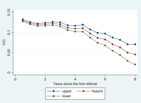
Kaplan–Meier hazard function with 95% confidence intervals
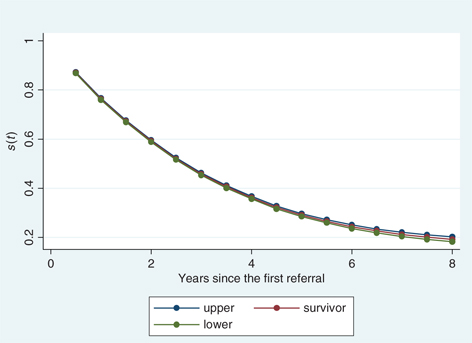
Kaplan–Meier survivor function with 95% confidence intervals
4 Data
This study used a large database of juvenile activity for Pennsylvania collected and maintained by the Center for Juvenile Justice Training and Research (CJJTR). The CJJTR is part of the Juvenile Court Judges’ Commission (JCJC), created in 1959 by the Pennsylvania Legislature. The JCJC is responsible for advising juvenile courts on court procedures and care of delinquents, overseeing administrative practices in probation offices, and collecting and reporting juvenile court statistics. For each year, the CJJTR collects and compiles data, which are initially entered by the juvenile court in each of Pennsylvania’s 67 counties, on each juvenile referred to the juvenile court system of Pennsylvania.[3] A juvenile may be referred to the court by police, school, probation officer, relative, social agency, another juvenile court, or district justice.
For every juvenile record, there was information on charges filed, whether the charges were substantiated, and outcome at disposition. Along with these variables there was information on juvenile’s race, age, ethnicity (Hispanic or non-Hispanic), county of residence, family status (whether the juvenile’s parents were currently married, divorced, separated, never married, or one or both deceased), and living arrangements (whether the juvenile was living with both parents, mother, father, relative, father and stepmother, mother and stepfather, or foster parents). We supplemented the original data set with variables on the juvenile’s county of residence that may affect recidivism: the number of police officers per capita, real income per capita, welfare payments per capita,[4] and population density.
The period of analysis was 1997–2005, with the data set containing 74,684 observations. The mean age of first referral to the juvenile court system was 15.4 for males and 15.6 for females. The minimum age was as low as 10.5 for males and 8.6 for females. 49.8% of male juveniles, and 31.7% of females in our data set were observed to have a second referral. This is not unusual; Cottle, Lee, and Heilbrun (2001), in a meta-analysis of 17 studies of juvenile recidivism, found that the mean recidivism rate was 48%, and a report by the Justice Department states that the conditional probability of a second referral was 59%.[5] The average time between the first and second referrals was 1.32 years for females and 1.34 years for males. Our explanatory variables, consisting primarily of dummy variables, include race and gender (white, black, and male), the age of the juvenile at the time of his first referral, his family characteristics (whether he lived with his mother, whether at least one parent was deceased), whether he was in school at the time of his first referral, and if so, the type of school, with dummy variables for special education and alternative education. Being male has been found to be a stable predictor of recidivism (Cottle, Lee, and Heilbrun 2001), although a trend of increasing offenses by females has been reported (Cottle, Lee, and Heilbrun 2001; Office of Juvenile Justice 2006); accordingly, we included an interaction term for male and year of first referral. Juveniles not attending school may have less supervision and more opportunities to commit crime. Students in special education programs who are gifted or handicapped may have lower rates of recidivism, while students in alternative education programs may have higher rates of recidivism in view of their past behavioral problems.
Other variables indicated the characteristics and judicial outcome of the first offense (whether the offense was a felony, and the severity of the punishment: whether the outcome of the case was merely a warning, or at the other extreme, a decision that the juvenile should be placed outside his home). A juvenile offender who receives only a warning may be more likely to commit another crime. On the other hand, the judge may have determined that it was appropriate to give the juvenile a warning because he is remorseful, and less likely to commit another offense. Conversely, a judicial decision that the juvenile should be placed outside his home, a relatively severe penalty, may deter him from future crimes. On the other hand, the severity of the sanction, or a conviction of a felony, could indicate that the juvenile’s first offense was more serious, suggesting that he is more likely to revert to antisocial behavior. Another variable indicated whether the juvenile was represented by a private attorney at the time of the first offense. Juveniles represented by private attorneys generally come from more prosperous households, which may affect recidivism. We included variables for the characteristics of the juvenile’s community: the real income per capita of his county of residence, welfare payments per capita, police per capita, a dummy variable for Philadelphia, the largest city in the state, and whether the county was classified as rural.[6] Counties with more police per capita might be more effective in deterring delinquent behavior, on the one hand, or more likely to apprehend offenders, on the other. Finally, we included variables for the year of the juvenile’s first referral and its square, in order to capture any trend in delinquent behavior. Table 1 shows the mean and standard deviation of these variables.
Mean of variables (n = 74,684)
| Variable | Mean |
| Were observed to have a second referral | 0.4564 (0.498) |
| In school | 0.788 (0.408) |
| Special education | 0.0046 (0.0676) |
| Alternative education | 0.0035 (0.0591) |
| At least one deceased parent | 0.0481 (0.214) |
| Lived with mother | 0.441 (0.497) |
| Had a private attorney at first referral | 0.0796 (0.271) |
| County real income per capita/100,000 | 0.3293 (0.0730) |
| Court disposition = warning | 0.081 (0.273) |
| Age at time of first referral | 15.45 (1.85) |
| White | 0.5967 (0.491) |
| Black | 0.3588 (0.480) |
| Male | 0.7723 (0.419) |
| Court disposition = placement outside the home | 0.0889 (0.285) |
| Felony | 0.1684 (0.374) |
| County of residence is rural | 0.2288 (0.420) |
| Philadelphia | 0.177 (0.382) |
| Year* = (year – 1997)/10 | 0.5234 (0.262) |
| Year* squared | 0.3424 (0.236) |
| Total police per capita × 1,000 | 2.19 (1.29) |
| Male × year* | 0.3905 (0.316) |
| Temporary Assistance to Needy Families per capita/100 | 0.6348 (0.733) |
| Time to second referral in years, if there was one | 1.340 (1.186) |
| Period of observation in years | 1.623 (1.368) |
5 Results
Results are set forth in Tables 2 and 3. Table 2 shows the effects of variables on the probability that a second referral will occur, while Table 3 shows their effects on the time to the second referral, conditional on the occurrence of that event. Some variables are significant in determining both the event of a second referral and the duration of time from first to second referral; some are significant in neither respect, and some are significant in one respect but not the other. These results are quite robust across the two specifications. The log-likelihood statistics indicate that the alternative model, positing a log-logistic distribution for the time to the second referral, fits the data somewhat better. However since the estimated coefficients of the two models are quite similar, we focus on the Schmidt–Witte specification, since that seems to have been used more often in studies of recidivism. To compute marginal effects, we used the Schmidt–Witte estimates in column 2. With regard to the estimates for the alternative model in column 5, note that gamma is estimated to be 0.6263, confirming that the underlying hazard of the log-logistic model rises and then falls. As to why it rises, it could be that a juvenile is less likely to commit an offense for some time after his first referral because of its deterrent effect, which may fade with time. The explanation cannot be that the juvenile is incarcerated, because as Table 1 shows, less than 9% of juveniles are sentenced to placement outside the home.
Effect of variables on a second referral (n = 74,684)
| Variable | Schmidt–Witte model | Alternative model | ||||
| Coefficient | Standard error | P-Value | Coefficient | Standard error | P-Value | |
| Intercept | 23.6076 | 0.4180 | 0.0000 | 13.4392 | 0.2254 | <0.0001 |
| In school | –0.5069 | 0.0386 | <0.0001 | –0.2780 | 0.0212 | <0.0001 |
| Special education | –1.2109 | 0.3476 | 0.0005 | –0.6896 | 0.1862 | 0.0002 |
| Alternative education | –0.1187 | 0.2578 | 0.6543 | –0.0989 | 0.1449 | 0.4948 |
| At least one deceased parent | 0.5667 | 0.0778 | <0.0001 | 0.3305 | 0.0435 | <0.0001 |
| Lives with mother | 0.2170 | 0.0330 | <0.0001 | 0.1198 | 0.0182 | 0.000 |
| Had private attorney | –0.3560 | 0.0599 | <0.0001 | –0.1933 | 0.0330 | <0.0001 |
| Real income per capita | –2.7273 | 0.2913 | <0.0001 | –1.3003 | 0.1590 | <0.0001 |
| Disposition warning | 0.0243 | 0.0600 | 0.6860 | 0.0460 | 0.0333 | 0.1678 |
| Age at first referral | –1.2174 | 0.0201 | <0.0001 | –0.6956 | 0.0107 | <0.0001 |
| White | 0.9220 | 0.0733 | <0.0001 | 0.5270 | 0.0404 | <0.0001 |
| Black | 0.5828 | 0.0747 | <0.0001 | 0.3431 | 0.0414 | 0.000 |
| Male | 0.8044 | 0.1239 | <0.0001 | 0.4977 | 0.0697 | <0.0001 |
| Disposition placement | 0.5984 | 0.0581 | <0.0001 | 0.3726 | 0.0334 | <0.0001 |
| Felony | 0.4074 | 0.0441 | <0.0001 | 0.2373 | 0.0248 | <0.0001 |
| Rural county of residence | –0.2282 | 0.0506 | <0.0001 | –0.1023 | 0.0276 | 0.0002 |
| Philadelphia | –0.9778 | 0.1511 | <0.0001 | –0.4506 | 0.0836 | <0.0001 |
| Year | –11.5708 | 0.5023 | <0.0001 | –6.9160 | 0.2836 | <0.0001 |
| Year squared | 6.1150 | 0.4728 | <0.0001 | 3.8183 | 0.2660 | <0.0001 |
| Total police per capita | 0.0696 | 0.0319 | 0.0292 | 0.0302 | 0.0169 | 0.0750 |
| Male × year | –0.1749 | 0.2247 | 0.4364 | –0.2146 | 0.1233 | 0.0818 |
| Welfare per capita | 0.5188 | 0.0815 | <0.0001 | 0.2826 | 0.0456 | <0.0001 |
Effect of variables on time to second referral, conditional on that event (n = 74684)
| Variable | Schmidt–Witte model | Alternative model | ||||
| Coefficient | Std error | P-Value | Coefficient | Std error | P-Value | |
| Intercept | 4.2947 | 0.0889 | <0.0001 | 4.4448 | 0.0790 | <0.0001 |
| In school | –0.1146 | 0.0164 | <0.0001 | –0.0984 | 0.0142 | <0.0001 |
| Special education | 0.2772 | 0.1471 | 0.0595 | 0.2159 | 0.1259 | 0.0863 |
| Alternative education | –0.3298 | 0.1125 | 0.0034 | –0.2870 | 0.0994 | 0.0039 |
| At least one deceased parent | –0.0661 | 0.0276 | 0.0165 | –0.0416 | 0.0241 | 0.0838 |
| Lives with mother | –0.0442 | 0.0138 | 0.0013 | –0.0470 | 0.0120 | 0.0001 |
| Had private attorney | 0.0399 | 0.0265 | 0.1325 | 0.0502 | 0.0228 | 0.0276 |
| Real income per capita | –0.5106 | 0.1378 | 0.0002 | –0.0985 | 0.1191 | 0.4081 |
| Disposition warning | –0.2942 | 0.0254 | <0.0001 | –0.2005 | 0.0227 | <0.0001 |
| Age at first referral | –0.2525 | 0.0038 | <0.0001 | –0.2707 | 0.0034 | <0.0001 |
| White | 0.0421 | 0.0363 | 0.2468 | 0.0543 | 0.0319 | 0.0889 |
| Black | –0.0213 | 0.0360 | 0.5535 | –0.0027 | 0.0315 | 0.9330 |
| Male | –0.0239 | 0.0330 | 0.4682 | –0.0209 | 0.0288 | 0.4675 |
| Disposition placement | 0.0206 | 0.0216 | 0.3380 | 0.1309 | 0.0190 | <0.0001 |
| Felony | –0.0956 | 0.0170 | <0.0001 | –0.0676 | 0.0148 | <0.0001 |
| Rural county of residence | –0.1223 | 0.0223 | <0.0001 | –0.0671 | 0.0194 | 0.0005 |
| Philadelphia | –0.0161 | 0.0615 | 0.7940 | 0.2061 | 0.0533 | 0.0001 |
| Year | –0.6847 | 0.1207 | <0.0001 | –0.5121 | 0.1065 | <0.0001 |
| Year squared | 1.3517 | 0.1340 | <0.0001 | 0.9596 | 0.1206 | <0.0001 |
| Total police per capita | –0.0410 | 0.0149 | 0.0058 | –0.0460 | 0.0126 | 0.0003 |
| Male × year | 0.0325 | 0.0769 | 0.6726 | –0.0180 | 0.0688 | 0.7933 |
| Welfare per capita | –0.0998 | 0.0262 | 0.0001 | –0.1287 | 0.0232 | <0.0001 |
| Gamma | 0.6263 | 0.0110 | <0.0001 | |||
| Sigma | 1.2116 | 0.00003 | <0.0001 | |||
| n | 74,684 | 74,684 | ||||
| Mean log-likelihood | –0.993662 | –0.873394 | ||||
Table 2 indicates that a juvenile who was in school, or in special education, at the time of his first offense, is less likely to revert to crime than one who was not in school. Others have found that school attendance has a negative effect on recidivism (Myner et al. 1998, Towberman 1994). We find that being in special education reduces the probability of a second referral by 26.1%, evaluating other variables at the mean. This finding conflicts with previous research finding that a history of special education increased the likelihood of recidivism (Archwamety and Katsiyannis 1998; Katsiyannis and Archwamety 1997). Moreover, it seems unlikely that this is attributable to different definitions of special education, since we find that alternative education does not have a significant effect.
A juvenile with at least one deceased parent, or who lives with his mother but without a father or stepfather, is more likely to have a second referral. Wadsworth (1979) found that delinquency was linked with the early loss of a parent through death or separation, and others have found such an effect of having a single parent (Cottle, Lee, and Heilbrun 2001). An individual from a relatively prosperous county, as measured by income per capita, or is represented by a private attorney, which suggests a higher family income, is less likely to revert to crime. Conversely, residence in a county with more welfare payments per capita increases the likelihood of recidivism. A second referral is more likely for juveniles in counties with more police per capita, presumably because the probability of apprehension is greater. Being younger at the time of first referral substantially increases one’s chance of recidivism, in accordance with the findings of many studies (Dembo et al. 1991; Ganzer and Sarason 1973; Hanson et al. 1984; Wierson and Forehand 1995; Tolan and Lorion 1988; Myner et al. 1998). Our estimates indicate that being a year older than the mean age of 15.4 years reduces the probability of a second referral by 26.3%, ceteris paribus. Being male increases the risk of recidivism by 13.1%. The estimates indicated that whites were more likely to have a relapse than others (blacks and the reference category, the aggregate of Hispanic and “other” races). Indeed the conditional probability of a second referral for whites was 16.1% greater than the reference category. Since this result was unexpected from the literature, we re-estimated the full model, but with the racial variables black, Hispanic, and “other races,” leaving white as the reference category. This yielded highly significant coefficients of –0.3052 for blacks, 0.5192 for Hispanics, and –1.059 for other races. Thus Hispanics are more likely to have a second referral than whites.
Living in a rural county reduces the risk of recidivism, but on the other hand so does residence in Philadelphia, the state’s biggest city. Thus recidivism seems to be most likely in suburbs and smaller cities. The estimated coefficients on the year of the first referral and year squared indicate that the probability of a second referral declined between 1997 and 2005, suggesting that Pennsylvania youths who entered the juvenile court system became more susceptible to rehabilitation over time, either because of a change in their characteristics or because methods of rehabilitation improved. With regard to the judicial outcome variables, placement outside the home seems to have had a perverse effect of increasing recidivism relative to other dispositions (a fine, probation, consent decree, transfer to adult criminal court, or informal resolution), but this may simply reflect sample selection bias. However Moore and Arthur (1989) suggested that out-of-home placement could lead to recidivism. A felony conviction at the first referral also increases one’s risk, which is consistent with the notion that more serious offenses are more likely to lead to future crimes. Severity of crime has often been cited as predicting recidivism (see, e.g. Wierson and Forehand 1995).
Table 3 shows the effects of variables on the time to the second referral, conditional on the occurrence of that event. Some variables that are estimated to increase the probability of a second referral also reduce the time to that event; this holds true for a felony conviction, having at least one deceased parent, living with one’s mother, and residence in a county with a higher incidence of welfare payments or more police per capita. As one would expect, a variable (special education) that reduces the probability of a second referral also increases the time to a second referral. However, some variables that reduce the probability of a second referral are estimated to reduce the time to that event, given that it occurs; this holds for the juvenile’s age at first referral, being in school, real income per capita, and living in a rural area. The coefficients on the age to first referral indicate that a youth who has his first referral when older is less likely to have a relapse, but also that he will get in trouble again sooner, given that he does so eventually. This does not seem unreasonable, given that older children have more mobility and freedom. Similarly, youths in school are less likely to revert to criminal behavior, but if they do, the close monitoring of them makes it likely that they will return to the juvenile justice system sooner.
6 Prediction of recidivism
After obtaining estimates from the full data set, following the practice of Schmidt and Witte (1989) and Berk et al. (2009), we split the sample into an analysis or estimation sample, used to obtain estimates of parameters, and a validation sample, used to test predictions of the model. The analysis sample and the validation sample have 70,641 and 4,043 observations, respectively. The estimation sample was chosen via application of a random number generator. Since one of our aspirations is to assist juvenile court judges by identifying those juveniles with the greatest risk of recidivism ex ante (before the judge’s determination), we eliminated the two variables indicating the judge’s decision (disposition warning and disposition placement). The idea is that the judge who is about to sentence a juvenile knows, or in principle could know, the values of all the variables in Tables 2 and 3 except the two variables for the disposition made by the court. The judge cannot know them because that decision has not yet been made; that is the decision he himself must make when he sentences the juvenile.
The coefficient estimates, which are quite similar to those derived from the full data set, are reported in Tables 6 and 7 in the Appendix. Thus the difference between Tables 2 and 3 and Tables 6 and 7 is that the latter (1) exclude 4,043 observations which are used to test their predictions and (2) do not include the two variables disposition warning and disposition placement.
In the analysis sample of 70,641 observations in Tables 6 and 7, there were 32,282 juveniles who had a second referral, or 45.7%. Again following Schmidt and Witte, we predict recidivism via the logit estimates for the same proportion of juveniles in the validation sample, 1,848 of 4,043 observations. Accordingly we took the top 1,848 observations in terms of probability of eventual failure, to learn how many of them were observed to have a second referral. It turns out that 1,434 of them, or 77.6%, did. Of the remaining 2,195, who would logically be predicted not to fail, only 371 did in fact fail. Thus our estimates have a false positive rate of 22.4% and a false negative rate of 16.9%. This is quite respectable. Schmidt and Witte, predicting recidivism of adult offenders in North Carolina with different variables, had a false positive rate of 47.2% and a false negative rate of 27.7%, which was far more accurate than the predictions of other models at the time. We also examined the top 20% of all observations in the validation sample in terms of predicted probability of eventual failure. We found that 748 of the 809 in this group, or 92.5%, were observed to have a second referral. Of the remainder, the failure rate was 32.7%. Finally, we examined the top 5% of observations in terms of predicted probability of eventual failure. We found that 171 of the 202 in this group, or 84.7%, were observed to have a second referral, and 42.5% of the remainder failed. Thus the model’s predictions did not strictly improve with the percentile of the sample.
| Recidivists | Non-recidivists | False positive rate (%) | False negativerate (%) | |
| Entire validation sample | 1,434 | 414 | 22.4 | 16.9 |
| Top 20% of predicted failures | 748 | 61 | 7.5 | 32.7 |
| Top 5% of predicted failures | 171 | 31 | 15.3 | 42.5 |
| Recidivists | Non-recidivists | False positive rate (%) | False negative rate (%) | |
| With race variables | ||||
| Entire validation sample | 17,712 | 5,033 | 22.1 | 18.5 |
| Top 20% of predicted failures | 9,243 | 714 | 7.2 | 33.8 |
| Top 5% of predicted failures | 2,201 | 288 | 11.6 | 43.4 |
| Without race variables | ||||
| Entire validation sample | 17,660 | 5,085 | 22.4 | 18.7 |
| Top 20% of predicted failures | 9,226 | 731 | 7.3 | 33.9 |
| Top 5% of predicted failures | 2,197 | 292 | 11.7 | 43.4 |
We considered that there might be legal difficulties – in particular claims of discrimination – if judges or other personnel in the juvenile justice system used personal demographic characteristics as a factor in predicting recidivism and thus in sentencing.[7] Accordingly we eliminated racial characteristics from the Schmidt–Witte model to see how that would affect its predictive power. Accordingly, we tested the predictive power of two models: one which employs the variables used in Table 1, but instead of just two racial variables has dummy variables for black, Hispanic, and “other race,” i.e. race other than black, white or Hispanic; and another model which is identical except that it has no variables for race. The parameters of both models were estimated on an analysis sample of 24,895 observations, and their predictions were tested on a validation sample of 49,787 observations. Since this analysis sample had 11,373 recidivists, we assumed that the number of failures in the validation sample would be approximately 45.7% of 49,787, or 22,745. The estimates of these models are presented in Tables 8 and 9 in the Appendix. They will be seen to be very similar to the estimates of Tables 6 and 7. Table 5 summarizes their predictive accuracy alternatively for (1) the entire validation sample, (2) those persons whose estimated probability of recidivism was in the highest 20%, and (3) those in the highest 5%.[8] The table shows that the false positive rate for out-of-sample prediction without the race variables is only slightly higher than prediction with the race variables, suggesting that race is a relatively insignificant factor in predictions of juvenile recidivism.
7 Summary and conclusion
This study uses a large database to analyze the factors affecting juvenile recidivism. We employ two different specifications of a split-population duration model to determine the effect of covariates on (1) the probability of eventual failure and (2) the time to failure, given that it occurs. The results are quite robust across the two specifications. With regard to the probability of a second offense, our findings generally confirm those of previous studies, with respect to variables like a felony conviction, the age of the juvenile at the time of first referral, being in school, and having a deceased parent. We found that a juvenile with at least one deceased parent, or one who lives with his mother but without a father or stepfather, is more likely to have a second referral. These findings have policy implications; they suggest that special attention should be given to juveniles who live with their mother only or who have at least one deceased parent. More frequent contact with a probation officer may be required because parental oversight for these juveniles may be less than for juveniles living in traditional family arrangements. It may also be helpful to reduce the case loads of probation officers assigned to juveniles who live in nontraditional families so that they can interact more closely with these at-risk juveniles.
Our variables for socioeconomic status are different from those of earlier studies, and perhaps somewhat less subject to criticism for measurement error or for being subjective: the variables for the juvenile’s community being county real income per capita, Temporary Assistance to Needy Families per capita, police per capita, and a variable at the individual level, having a private attorney. All these variables indicate that a juvenile from a more prosperous family, or a more affluent community, is less likely to have a relapse. Two coefficient estimates that are atypical are those of special education, which reduces the probability of recidivism by 26%, and being white, which increases it by 16%.
Finally, we test the predictive power of our estimates from the Schmidt–Witte model. Our estimates have a false positive rate of 18.5% and a false negative rate of 20.7%. We would argue that the accuracy of these results justifies taking estimates from this model into account both in sentencing and in deciding how to monitor and follow up on the juveniles predicted to have the highest probabilities of recidivism. If the false positive rate is considered too high to use the estimates as the basis for a recommended sentence, further research and refinement of this model could make its implementation acceptable.
Appendix I: when juveniles are excluded from juvenile court jurisdiction
Pennsylvania’s Act 33 of 1996 created conditions in which a juvenile under age 18 could be excluded from juvenile court jurisdiction. Prior to Act 33 only juveniles charged with murder were excluded from the juvenile court’s jurisdiction. Under Act 33 juveniles could now be excluded if they were aged 15 or older and charged certain violent crimes (e.g. aggravated assault, rape, murder, robbery, kidnapping). In addition, the juvenile must either have used a deadly weapon or have previously been adjudicated to have committed one of the excluded offenses. Even if there is prima facie case and the exclusion criteria are met, it is possible that some cases may return to juvenile court following a decertification hearing in criminal court whereby a juvenile files a request that the case be tried in juvenile court. As a result of the foregoing exclusions, the data set used in this study did not contain information on juveniles who committed some of the most violent crimes, and this will lead to an underreporting of recidivism, but this omission was a minor problem since the number of juveniles excluded from juvenile court was small. In 1996, only 473 cases were excluded from juvenile jurisdiction, leading to 109 convictions in criminal court.
Appendix II: Tables 6–9
Effect of variables on a second referral (n = 70,641)
| Variable | Schmidt–Witte model | Alternative model | ||||
| Coefficient | Standard error | P-Value | Coefficient | Standard error | P-Value | |
| Intercept | 23.7726 | 0.4323 | <0.0001 | 13.541 | 0.2331 | <0.0001 |
| In school | –0.5106 | 0.0398 | <0.0001 | –0.2795 | 0.0219 | <0.0001 |
| Special education | –1.1231 | 0.3507 | 0.0014 | –0.6413 | 0.1905 | 0.0008 |
| Alternative education | –0.2982 | 0.2623 | 0.2557 | –0.1851 | 0.1484 | 0.2124 |
| At least one deceased parent | 0.5663 | 0.0800 | <0.0001 | 0.3308 | 0.0449 | <0.0001 |
| Lives with mother | 0.2229 | 0.0340 | <0.0001 | 0.1242 | 0.0188 | <0.0001 |
| Had private attorney | –0.3342 | 0.0617 | <0.0001 | –0.1796 | 0.0341 | <0.0001 |
| Real income per capita | –2.8022 | 0.2970 | <0.0001 | –1.3347 | 0.1602 | <0.0001 |
| Age at first referral | –1.2260 | 0.0208 | <0.0001 | –0.7023 | 0.0111 | <0.0001 |
| White | 0.9455 | 0.0758 | <0.0001 | 0.5450 | 0.0419 | <0.0001 |
| Black | 0.6113 | 0.0772 | <0.0001 | 0.3625 | 0.0429 | <0.0001 |
| Male | 0.8268 | 0.1277 | <0.0001 | 0.5228 | 0.0716 | <0.0001 |
| Felony | 0.4984 | 0.0444 | <0.0001 | 0.2923 | 0.0250 | <0.0001 |
| Rural county of residence | –0.2502 | 0.0516 | <0.0001 | –0.1171 | 0.0281 | <0.0001 |
| Philadelphia | –0.9049 | 0.1554 | <0.0001 | –0.4153 | 0.0862 | <0.0001 |
| Year | –11.4907 | 0.5193 | <0.0001 | –6.8248 | 0.2898 | <0.0001 |
| Year squared | 6.0723 | 0.4888 | <0.0001 | 3.7879 | 0.2732 | <0.0001 |
| Total police per capita | 0.0787 | 0.0331 | 0.0174 | 0.0352 | 0.0177 | 0.0468 |
| Male × year | –0.2242 | 0.2311 | 0.3320 | –0.2612 | 0.1270 | 0.0397 |
| Welfare per capita | 0.4792 | 0.0840 | <0.0001 | 0.2627 | 0.0470 | <0.0001 |
Effect of variables on time to second referral, conditional on that event
| Variable | Schmidt–Witte model | Alternative model | ||||
| Coefficient | Standard error | P-Value | Coefficient | Standard error | P-Value | |
| Intercept | 4.2485 | 0.0915 | <0.0001 | 4.3738 | 0.0789 | <0.0001 |
| In school | –0.1002 | 0.0169 | <0.0001 | –0.0823 | 0.0146 | <0.0001 |
| Special education | 0.2763 | 0.1467 | 0.0596 | 0.2268 | 0.1261 | 0.0720 |
| Alternative education | –0.3493 | 0.1156 | 0.0025 | –0.2933 | 0.1025 | 0.0042 |
| At least one deceased parent | –0.0596 | 0.0284 | 0.0357 | –0.0355 | 0.0248 | 0.1529 |
| Lives with mother | –0.0424 | 0.0142 | 0.0028 | –0.0442 | 0.0124 | 0.0003 |
| Had private attorney | 0.0455 | 0.0273 | 0.0954 | 0.0568 | 0.0235 | 0.0157 |
| Real income per capita | –0.3648 | 0.1411 | 0.0097 | –0.0140 | 0.1011 | 0.8897 |
| Age at first referral | –0.2559 | 0.0039 | <0.0001 | –0.2705 | 0.0035 | <0.0001 |
| White | 0.0460 | 0.0378 | 0.2245 | 0.0654 | 0.0343 | 0.0562 |
| Black | –0.0207 | 0.0375 | 0.5812 | 0.0074 | 0.0341 | 0.8283 |
| Male | –0.0184 | 0.0334 | 0.5813 | –0.0115 | 0.0297 | 0.6982 |
| Felony | –0.0686 | 0.0171 | 0.0001 | –0.0315 | 0.0149 | 0.0388 |
| Rural county of residence | –0.1012 | 0.0229 | <0.0001 | –0.0588 | 0.0191 | 0.0021 |
| Philadelphia | 0.0693 | 0.0630 | 0.2715 | 0.2739 | 0.0548 | <0.0001 |
| Year | –0.6761 | 0.1236 | <0.0001 | –0.5133 | 0.1095 | <0.0001 |
| Year squared | 1.3534 | 0.1379 | <0.0001 | 0.9888 | 0.1242 | <0.0001 |
| Total police per capita | –0.0377 | 0.0152 | 0.0135 | –0.0426 | 0.0129 | 0.0010 |
| Male × year | 0.0208 | 0.0776 | 0.7883 | –0.0317 | 0.0706 | 0.6533 |
| Welfare per capita | –0.1301 | 0.0270 | <0.0001 | –0.1544 | 0.0239 | <0.0001 |
| Sigma | 1.2149 | 0.00003 | <0.0001 | |||
| Gamma | 0.62876 | 0.0113 | <0.0001 | |||
| n | 70,641 | 70,641 | ||||
| Mean log-likelihood | –0.99620 | –0.876250 | ||||
Effect of variables on a second referral, with and without race variables (n = 24,895)
| Variable | Schmidt–Witte model with race variables | Schmidt–Witte model without race variables | ||||
| Coefficient | Standard error | P-Value | Coefficient | Standard error | P-Value | |
| Intercept | 22.957 | 0.6686 | <0.0001 | 23.2308 | 0.6719 | <0.0001 |
| In school | –0.5448 | 0.0647 | <0.0001 | –0.5110 | 0.0646 | <0.0001 |
| Special education | –1.6654 | 0.5874 | 0.0046 | –1.6465 | 0.5931 | 0.0055 |
| Alternative education | –0.2230 | 0.4368 | 0.6096 | –0.2357 | 0.4425 | 0.5942 |
| At least one deceased parent | 0.5857 | 0.1258 | <0.0001 | 0.5950 | 0.1257 | <0.0001 |
| Lives with mother | 0.2831 | 0.0556 | <0.0001 | 0.2811 | 0.0552 | <0.0001 |
| Had private attorney | –0.3323 | 0.0995 | 0.0008 | –0.3255 | 0.0995 | 0.0011 |
| Real income per capita | –3.1078 | 0.4813 | <0.0001 | –3.6163 | 0.4731 | <0.0001 |
| Disposition warning | 0.0009 | 0.1154 | 0.9941 | –0.0234 | 0.1024 | 0.8195 |
| Age at first referral | –1.1420 | 0.0319 | <0.0001 | –1.1492 | 0.0319 | <0.0001 |
| Hispanic | 0.5935 | 0.1476 | 0.0001 | |||
| Black | –0.185 | 0.0668 | 0.0056 | |||
| Other race | –1.1211 | 0.1294 | <0.0001 | |||
| Male | 0.7863 | 0.2156 | 0.0003 | 0.8054 | 0.2110 | 0.0001 |
| Disposition placement | 0.6525 | 0.0962 | <0.0001 | 0.6449 | 0.0960 | <0.0001 |
| Felony | 0.3457 | 0.0747 | <0.0001 | 0.3414 | 0.0747 | <0.0001 |
| Rural county of residence | –0.1294 | 0.0863 | 0.1341 | –0.2080 | 0.0853 | 0.0148 |
| Philadelphia | –1.4966 | 0.2531 | <0.0001 | –1.5457 | 0.2525 | <0.0001 |
| Year | –10.9617 | 0.8345 | <0.0001 | –11.1377 | 0.8388 | <0.0001 |
| Year squared | 5.5919 | 0.7716 | <0.0001 | 5.8035 | 0.7785 | <0.0001 |
| Total police per capita | 0.1587 | 0.0534 | 0.0030 | 0.1463 | 0.0530 | 0.0057 |
| Male × year | –0.1077 | 0.3892 | 0.7819 | –0.1136 | 0.3805 | 0.7653 |
| Welfare per capita | 0.6206 | 0.1378 | <0.0001 | 0.5687 | 0.1366 | <0.0001 |
Effect of variables on time to second referral, conditional on that event: with and without race variables
| Variable | Schmidt–Witte model with race variables | Schmidt–Witte model without race variables | ||||
| Coefficient | Standard error | P-Value | Coefficient | Standard error | P-Value | |
| Intercept | 4.4027 | 0.1374 | <0.0001 | 4.4314 | 0.1378 | <0.0001 |
| In school | –0.1333 | 0.0280 | <0.0001 | –0.1329 | 0.0280 | <0.0001 |
| Special education | 0.3197 | 0.2279 | 0.1607 | 0.3230 | 0.2277 | 0.1560 |
| Alternative education | –0.4209 | 0.1984 | 0.0339 | –0.4127 | 0.1981 | 0.0372 |
| At least one deceased parent | –0.1114 | 0.0457 | 0.0148 | –0.1131 | 0.0458 | 0.0135 |
| Lives with mother | –0.0252 | 0.0236 | 0.2864 | –0.0315 | 0.0235 | 0.1789 |
| Had private attorney | 0.0497 | 0.0447 | 0.2660 | 0.0520 | 0.0448 | 0.2456 |
| Real income per capita | –0.6521 | 0.2322 | 0.0050 | –0.7942 | 0.2288 | 0.0005 |
| Disposition warning | –0.2438 | 0.0435 | <0.0001 | –0.2447 | ||
| Age at first referral | –0.2577 | 0.0064 | <0.0001 | –0.2557 | –0.2557 | <0.0001 |
| Hispanic | 0.0351 | 0.0522 | 0.501 | |||
| Black | –0.0695 | 0.0286 | 0.5812 | |||
| Other race | –0.1141 | 0.0657 | 0.0826 | |||
| Male | –0.0043 | 0.0561 | 0.9395 | –0.0024 | 0.0024 | 0.9673 |
| Disposition placement | –0.0022 | 0.0370 | 0.9530 | –0.0018 | 0.0369 | 0.9606 |
| Felony | –0.0415 | 0.0292 | 0.1559 | –0.0430 | 0.0293 | 0.1420 |
| Rural county of residence | –0.1122 | 0.0384 | 0.0035 | –0.1185 | 0.0381 | 0.0019 |
| Philadelphia | –0.0921 | 0.1043 | 0.3774 | –0.0679 | 0.1036 | 0.5121 |
| Year | –0.7785 | 0.2048 | 0.0001 | –0.7740 | 0.2061 | 0.0002 |
| Year squared | 1.3042 | 0.2269 | <0.0001 | 1.3140 | 0.2267 | <0.0001 |
| Total police per capita | –0.0189 | 0.0249 | 0.4462 | –0.0322 | 0.0244 | 0.1866 |
| Male × year | 0.0914 | 0.1322 | 0.4893 | 0.0915 | 0.1345 | 0.4964 |
| Welfare per capita | –0.0813 | 0.0444 | 0.0674 | –0.0994 | 0.0440 | 0.0239 |
| Sigma | 1.1896 | 0.0043 | <0.0001 | 1.1927 | 0.0043 | <0.0001 |
| n | 24,895 | 24,895 | ||||
| Mean log-likelihood | –0.99237 | –0.994057 | ||||
References
Archwamety, T., and A.Katsiyannis. 1998. “Factors Related to Recidivism Among Delinquent Females in a State Correctional Facility.” Journal of Child and Family Studies7(1):59–67.10.1023/A:1022960013342Search in Google Scholar
Archwamety, T., and A.Katsiyannis. 2000. “Academic Remediation, Parole Violations, and Recidivism Rates among Delinquent Youths.” Remedial and Special Education21(3):161–70.10.1177/074193250002100306Search in Google Scholar
Berk, R., L.Sherman, G.Barnes, E.Kurtz, and L.Ahlman. 2009. “Forecasting Murder within a Population of Probationers and Parolees: A High Stakes Application of Statistical Learning.” Journal of Royal Statistical Society (Series A)172(1):1–21.10.1111/j.1467-985X.2008.00556.xSearch in Google Scholar
Box-Steffensmeier, J. M., and B. S.Jones. 2004. Event History Modelling: A Guide for Social Scientists. New York: Cambridge University Press.10.1017/CBO9780511790874Search in Google Scholar
Brame, R., S. D.Bushway, and R.Paternoster. 2003. “Examining the Prevalence of Criminal Desistance.” Criminology41(2):423–48.10.1111/j.1745-9125.2003.tb00993.xSearch in Google Scholar
Bunday, B. D., and V. A.Kiri. 1992. “Analysis of Censored Recidivism Data Using a Proportional Hazards-Type Model.” The Statistician41(1):85–96.10.2307/2348639Search in Google Scholar
Cohen, L. E., and B. J.Vila. 1996. “Self-Control and Social-Control: An Exposition of the Gottfredson-Hirschi/Sampson-Laub Debate.” Studies on Crime and Crime Prevention5:125–50.Search in Google Scholar
Cottle, C. C., R. J.Lee, and K.Heilbrun. 2001. “The Prediction of Criminal Recidivism in Juveniles: A Meta-Analysis.” Criminal Justice and Behavior28(3):367–94.10.1177/0093854801028003005Search in Google Scholar
Dembo, R., L.Williams, J.Schmeidler, A.Getreu, and E.Berry. 1991. “Recidivism among High-Risk Youths: A 2 1/2-Year Follow-Up of a Cohort of Juvenile Detainees.” International Journal of the Addictions26:1197–221.10.3109/10826089109062155Search in Google Scholar
Dembo, R., L.Williams, J.Schmeidler, B.Nini-Gough, C. C.Sue, P.Borden, and D.Manning. 1998. “Predictors of Recidivism to a Juvenile Assessment Center: A Three-Year Study.” Journal of Child and Adolescent Substance Abuse7:57–77.10.1300/J029v07n03_03Search in Google Scholar
Douglas, S., and G.Hariharan. 1994. “The Hazard of Starting Smoking: Estimates From a Split Population Duration Model.” Journal of Health Economics13:213–30.10.1016/0167-6296(94)90024-8Search in Google Scholar
Escarela, G., B.Francis, and K.Soothill. 2000. “Competing Risks, Persistence, and Desistance in Analyzing Recidivism.” Journal of Quantitative Criminology16(4):385–414.10.1023/A:1007586031274Search in Google Scholar
Farrington, D. P. 1992. “Criminal Career Research in the United Kingdom.” British Journal of Criminology32:521–36.10.1093/oxfordjournals.bjc.a048255Search in Google Scholar
Forster, M., and A. M.Jones. 2001. “The Role of Tobacco Taxes in Starting and Quitting Smoking: Duration Analysis of British Data.” Journal of the Royal Statistical Society Series a (Statistics in Society)164(3):517–47.10.1111/1467-985X.00217Search in Google Scholar
Ganzer, V. J., and I. G.Sarason. 1973. “Variables Associated with Recidivism Among Juvenile Delinquents.” Journal of Consulting and Clinical Psychology40:1–5.10.1037/h0034012Search in Google Scholar
Hanson, C. L., S. W.Henggeler, W. F.Haefele, and J. D.Rodick. 1984. “Demographic, Individual and Family Relationship Correlates of Serious and Repeated Crime among Adolescents and Their Siblings.” Journal of Consulting and Clinical Psychology52:528–38.10.1037/0022-006X.52.4.528Search in Google Scholar
Katsiyannis, A., and T.Archwamety. 1997. “Factors Related to Recidivism Among Delinquent Youths in a State Correctional Facility.” Journal of Child and Family Studies6:43–55.10.1023/A:1025068623167Search in Google Scholar
Koopman, S. J., M.Ooms, A.Lucas, K.van Montfort, and V.van der Guest. 2008. “Estimating Systematic Continuous-Time Trends in Recidivism Using a Non-Gaussian Panel Datamodel.” Statistica Neerlandica62(1):104–30.10.1111/j.1467-9574.2007.00375.xSearch in Google Scholar
Mbuba, J. M. 2004. “Juvenile Recidivism: An Analysis of Race and Other Socio-Demographic Predictors within Three Intervention Modalities in the State of Louisiana.” Unpublished Ph.D. dissertation.Search in Google Scholar
Mbuba, J. M. 2005. “A Refutation of Racial Differentials in the Juvenile Recidivism Rate Hypothesis.” African Journal of Criminology & Justice Studies1(2):51–68.Search in Google Scholar
Moore, D. R., and J. L.Arthur. 1989. “Juvenile Delinquency.” In Handbook of Child Psychopathology, edited by T. H. Olendick and M. Hersen, 2nd ed., 197–217. New York: Plenum.10.1007/978-1-4757-1162-2_9Search in Google Scholar
Myner, J., J.Santman, G. G.Cappelletty, and B. F.Perlmutter. 1998. “Variables Related to Recidivism Among Juvenile Offenders.” International Journal of Offender Therapy and Comparative Criminology42(1):65–80.10.1177/0306624X98421006Search in Google Scholar
Nuttall, J., L.Hollmen, and E. M.Staley. 2003. “The Effect of Earning a GED on Recidivism Rates.” Journal of Correctional Education54(3):90–4.Search in Google Scholar
Office of Juvenile Justice and Delinquency Prevention, National Center for Juvenile Justice. 2006. Juvenile Offenders and Victims: 2006 National Report. Pittsburgh, PA.Search in Google Scholar
Paternoster, R., R.Brame, and D. P.Farrington. 2001. “On the Relationship between Adolescent and Adult Conviction Frequencies.” Journal of Quantitative Criminology17(3):201–25.10.1023/A:1011007016387Search in Google Scholar
Pezzin, L. 1995. “Earnings Prospects, Matching Effects, and the Decision to Terminate a Criminal Career.” Journal of Quantitative Criminology33(3):29–50.10.1007/BF02221299Search in Google Scholar
Putnins, A. 2003. “Substance Use and the Prediction of Young Offender Recidivism.” Drug Alcohol Review22(4):401–8.10.1080/09595230310001613912Search in Google Scholar
Puzzanchera, C. 2009. Juvenile Arrests 2008. Juvenile Justice. Bulletin. Washington, DC: Office of Juvenile Justice and. Delinquency Prevention).Search in Google Scholar
Rhodes, W. 1989. “The Criminal Career: Estimates of the Duration and Frequency of Crime Commission.” Journal of Quantitative Criminology5:3–32.10.1007/BF01066259Search in Google Scholar
Ryan, J. P., and H.Yang. 2005. “Family Contact and Recidivism: A Longitudinal Study of Adjudicated Delinquents in Residential Care.” Social Work Research29:31–39.10.1093/swr/29.1.31Search in Google Scholar
Schmidt, P., and A. D.Witte. 1989. “Predicting Criminal Recidivism Using ‘Split-Population’ Survival Time Models.” Journal of Econometrics40:141–59.10.1016/0304-4076(89)90034-1Search in Google Scholar
Tolan, P. H., and R. P.Lorion. 1988. “Multivariate Approaches to the Identification of Delinquency Proneness in Adolescent Males.” American Journal of Community Psychology16:547–61.10.1007/BF00922770Search in Google Scholar
Tollenaar, N., and P. G. M.van der Heijden. 2013. “Which Method Predicts Recidivism Best?: A Comparison of Statistical, Machine Learning and Data Mining Predictive Models.” Journal of the Royal Statistical Society: Series a (Statistics in Society176(2):565–84.10.1111/j.1467-985X.2012.01056.xSearch in Google Scholar
Towberman, D.1994. “Psychosocial Antecedents of Chronic Delinquency.” In Young victims, young offenders: Current issues in policy and treatment, edited by N. J.Pallone, 151–64. New York: Haworth.10.4324/9781315792897-10Search in Google Scholar
Wadsworth, M.. 1979. Roots of Delinquency. New York: Barnes and Noble).Search in Google Scholar
Wierson, M., and R.Forehand. 1995. “Predicting Recidivism in Juvenile Delinquents: The Role of Mental Health Diagnoses and the Qualification of Conclusions by Race.” Behavior Research and Therapy33:63–67.10.1016/0005-7967(94)E0001-YSearch in Google Scholar
Wolfgang, M. E., R. M.Figlio, and T.Sellin. 1972. Delinquency in a Birth Cohort. Chicago: The University of Chicago Press.Search in Google Scholar
©2015 by De Gruyter
Articles in the same Issue
- Frontmatter
- Advances
- Systematic Bailout Guarantees and Tacit Coordination
- On Cross-Border Mergers and Product Differentiation
- Contributions
- Fostering Household Formation: Evidence from a Spanish Rental Subsidy
- Parental Preferences for Primary School Characteristics
- Health Care Use, Out-of-Pocket Expenditure, and Macroeconomic Conditions during the Great Recession
- The Signaling Role of Subsidies
- Spillover Effects of Drug Safety Warnings on Preventive Health Care Use
- How Should Cartels React to Entry Triggered by Demand Growth?
- Topics
- Intergenerational Income Mobility in Taiwan: Evidence from TS2SLS and Structural Quantile Regression
- Pricing of First-Run Movies in Small U.S. Metropolitan Areas: Multimarket Contact and Chain Effects
- Minimum Wages: Do They Really Hurt Young People?
- Predicting Recidivism of Juvenile Offenders
- Religious Participation, Trust and Reciprocity: Evidence from Six Latin American Cities
- Vocational Training and Labor Market Outcomes in Brazil
- Do Charitable Subsidies Crowd Out Political Giving? The Missing Link between Charitable and Political Contributions