AlgDiff: an open source toolbox for the design, analysis and discretisation of algebraic differentiators
-
Amine Othmane

 and
Joachim Rudolph
and
Joachim Rudolph

Abstract
Algebraic differentiators have attracted much interest in recent years. Their simple implementation as classical finite impulse response digital filters and systematic tuning guidelines may help to solve challenging problems, including, but not limited to, nonlinear feedback control, model-free control, and fault diagnosis. This contribution introduces the open source toolbox AlgDiff for the design, analysis and discretisation of algebraic differentiators.
Zusammenfassung
Algebraische Ableitungsschätzer haben in den letzten Jahren großes Interesse erlangt. Dank ihrer einfachen Implementierung als klassische digitale Filter mit endlicher Impulsantwort und der systematischen Parametrierungsansätze können sie zur Lösung anspruchsvoller regelungstechnischer Probleme beitragen. Dieser Beitrag stellt die Open-Source-Toolbox AlgDiff für den Entwurf, die Analyse und die Diskretisierung algebraischer Ableitungsschätzer vor.
1 Introduction
Numerical estimation of derivatives of measured signals is a long-standing and challenging problem because small perturbations in the measurements may yield significant errors in the estimates. Numerous approaches have been proposed to address this problem: frequency-domain digital filter design [1, 2], Tikhonov regularisation [3, 4], observers design [5–9], local least-squares fitting of data by polynomials [10, 11], and differentiation by integration methods [12–14]. Algebraic differentiators have been proposed in [15, 16] and further discussed and extended in [17–25], for example. A detailed introduction to these differentiation techniques, their historical evolution, and links to established methods in the literature are summarised in the free-access survey [26].
Algebraic differentiators may be interpreted as differentiation by integration methods and may be implemented as classical finite impulse response (FIR) digital filters. The design of these differentiators involves the judicious choice of up to five parameters, which can be challenging. For example, it has been pointed out in [15, 16] that accepting a slight but known delay in the estimates reduces the order of the approximation error. In [23], it has been observed that delay-free differentiators may exhibit intolerable gains in their amplitude spectra.
Analysing the effects of the parameters on the frequency-domain properties has been very useful in deriving systematic tuning guidelines. In [21], it has been shown that it is possible to approximate the differentiators as low-pass filters. The tuning parameters can then be determined by specifying the desired cutoff frequency and stopband slope. Further effects of the parameters on the frequency-domain properties have been discussed in [22, 24, 25], for example. The simple implementation of these differentiators and their good robustness with respect to measurement disturbances has motivated their wide use. An extensive list of applications including but not limited to parameter estimation, fault detection and feedback control has been published in [26].
A first version of an open-source toolbox implementing all necessary functions for the design, analysis, and discretisation of algebraic differentiators has been made available with the survey [26]. The toolbox is implemented in Python. Numerous examples show how it can be used in Matlab. The toolbox [27] allows users to specify desired frequency-domain properties and estimating derivatives of signals in very few lines of code, for example. Time-domain and frequency-domain properties are automatically calculated and can be easily accessed. In the current contribution a step-by-step tutorial is provided for algebraic differentiators using this toolbox. Relevant properties are recalled and demonstrated. Discretisation effects and a special parametrisation for the exact annihilation of harmonic signals first discussed in [21] are also addressed using simple examples. The source code of the latter examples is made freely available in the toolbox repository for Python and Matlab.
This tutorial-like article is structured as follows. Section 2 describes the main features of the toolbox. Section 3 recalls the basics of algebraic differentiators required for the remaining parts. Section 4 constitutes the main part of this work and recalls the properties of algebraic differentiators in the light of the toolbox. Example code snippets are used to show how the different functions can be used. A short conclusion is provided in Section 5. Appendices A–E summarise explicit mathematical expressions related to algebraic differentiators that are provided for the sake of completeness.
2 The toolbox AlgDiff
The toolbox contains an implementation in Python for all necessary functions for the design, analysis, and discretisation of algebraic differentiators. The toolbox is available under the BSD-3-Clause License, making it suitable for academic and industrial/commercial use. An interface to Matlab is included in the package, and several use cases are documented. The repository also contains detailed documentation of the Python class and its methods. The prerequisites for using the toolbox are described in detail.
The repository also includes a graphical user interface (GUI) that further simplifies the design of algebraic differentiators. The GUI enables specifying desired time-domain and frequency-domain properties for the filters. Relevant properties like the approximation delay, the discretisation error, the cutoff frequency, and the filter window length are displayed. Numerical values for amplitude spectra, step responses, impulse responses, and filter coefficients can be exported. Different approaches can be used to discretise the differentiators. Measurement data can be loaded into the GUI and derivatives can then be easily computed. Figure 1 shows a screenshot of the GUI for a specific algebraic differentiator.
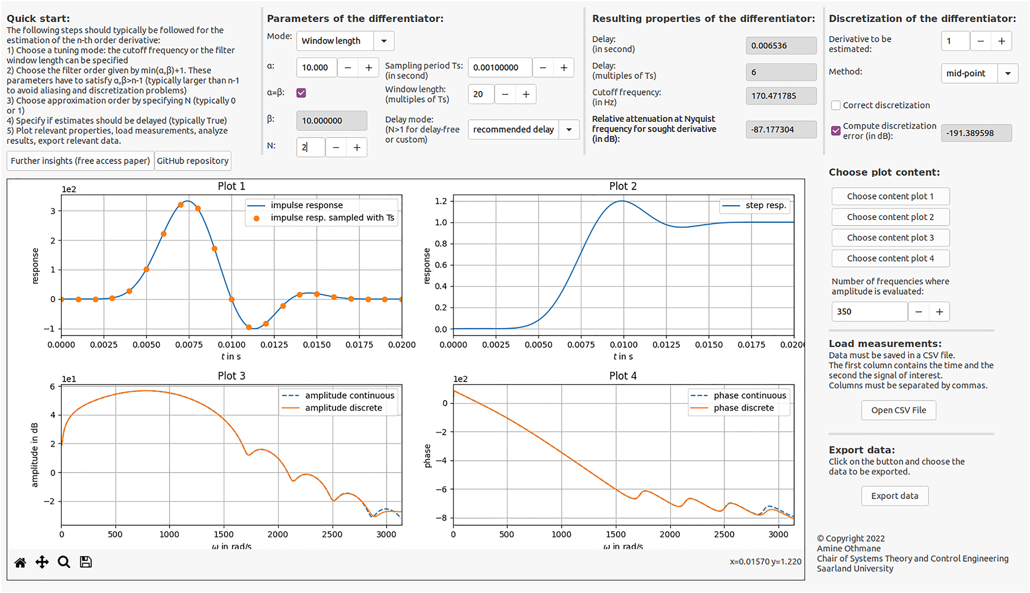
Screenshot of the GUI for a specific parametrisation of algebraic differentiators.
3 Background material on algebraic differentiators
This section provides a brief summary of the fundamentals of algebraic differentiators, which were originally developed in [15, 16]. A comprehensive survey on the existing results, interpretations, relationships to established methods, tuning guidelines, and applications can be found in [26].
3.1 Derivative estimation
While the early works [15, 16] use differential algebraic manipulations and operational calculus to derive the differentiators, later ones such as [20], [21], [22, 25, 28] use time-domain derivations. This shall be briefly recalled.
Let
with
The estimate
If ϑ corresponds to a zero of the polynomial
3.2 Interpretations
As discussed in [26], different interpretations can be attached to algebraic differentiators. Two important ones are recalled in Table 1. The approximation-theoretic interpretation stems from the time-domain derivation of the differentiators. It is helpful for the analysis of the approximation error and delays. The systems-theoretic interpretation is a direct consequence of the definition of the approximated derivative in (1): The estimate is the output of a linear time invariant filter where the kernel is the nth order derivative of
Extract from [26]: interpretations of
| Context | Interpretation | Practical usage |
|---|---|---|
| Approximation-theoretic | Polynomial approximation of derivative using a Hilbert reproducing kernel | Analysis of estimation properties and relation to established differentiation methods |
| Systems-theoretic | Linear time-invariant filtering of the sought derivative: | Analysis of filter properties and parametrisation |

|
||
| Linear time-invariant filtering of the measured signal: | Discretisation and implementation | |

|
4 Algebraic differentiators in the light of AlgDiff
This section reviews the properties of algebraic differentiators in the time and frequency domains and shows how the toolbox can be used to analyse these filters. First, the continuous-time differentiators are considered. Then, discretisation issues are discussed and functions of the toolbox that can be used to ensure that the discrete-time filter preserves the properties of the continuous-time ones are introduced. Finally, the estimation of the derivative of an example signal is considered. The code snippets provided in this section are written in Python to adhere to the open-source philosophy of the package. However, the repository contains the same examples also written for Matlab.
4.1 Impulse and step responses
The impulse and step responses of an algebraic differentiator
Example 1
(Impulse and step responses). The impulse and step responses of an algebraic differentiator with parameter α = 4, β = 4, N = 0, and T = 0.1 can be computed using the toolbox as shown in Code snippet 1.
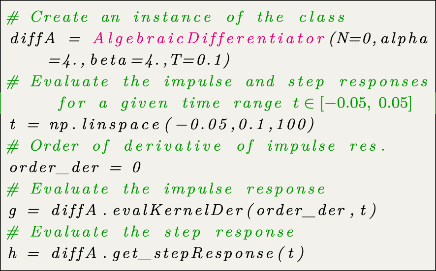
Evaluation of the impulse and step responses of an algebraic differentiator.
Figure 2 shows the impulse and step responses of algebraic differentiators for N = 0 and different values of α and β. It can be observed that increasing β and keeping α constant causes a stronger weighting of the impulse response towards 0. This increase implies a stronger weighting of more recent values of the sought derivative and corresponds to the reduction of the estimation delay. In contrast, increasing α and keeping β constant yields a stronger weighting of the impulse response in the direction of T, which leads to a stronger weighting of older values of the sought derivative and, thus, to an increase of the estimation delay. The effects of the parameters on the delay has been analysed analytically in [16, 20, 25, 26], for example.
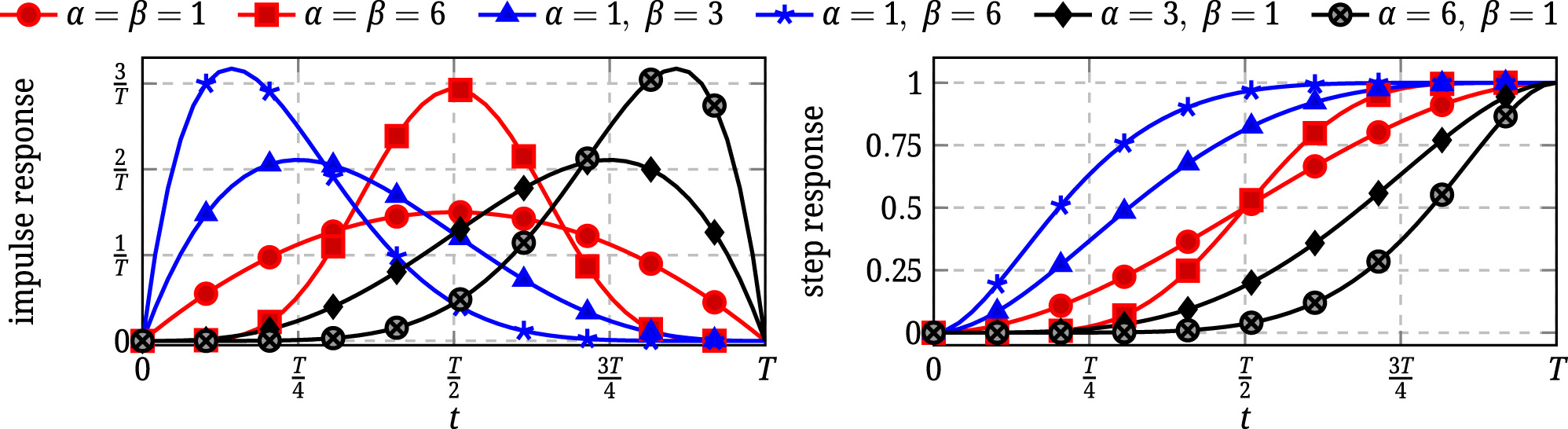
Impulse and step responses of algebraic differentiators with parameters α, β ∈ {1, 3, 6}, and N = 0.
The analytical properties of the impulse response and its derivatives can be used to derive tuning guidelines for fault detection algorithms, for example. Approaches have been developed and experimentally validated in [21, 22, 28, 30], for example.
4.2 Frequency-domain properties
By recalling that the estimate of the nth order derivative of y is a convolution product of the signal and the nth order derivative of the differentiator
with
Analysing
of the amplitude spectrum of an algebraic differentiator has been proposed in [21], where ω
c is defined in (A.11) and μ = 1 + min{α, β}. It follows that
Tuning guidelines proposed in [21, 22] can then be inferred from (2): A desired cutoff frequency ω c and a desired filter order, i.e., the stopband slope given by 20μ dB, can be specified. Then, the filter window length can be computed from (A.11).
It has been shown in [24–26] that increasing N increases the sensitivity to noise. It has also been shown in [24] that the choice α = β yields differentiators with maximum robustness to noise. In addition, according to [22, 25], and [26], choosing α ≠ β reduces stopband ripples in the amplitude spectrum.
Example 2 shows how a differentiator can be designed from desired frequency-domain properties using the toolbox. The computation of the amplitude and phase spectra is also demonstrated. Example 3 compares and discusses the amplitude spectrum of differentiators with and without delay.
Example 2
(Specifying frequency-domain properties). An algebraic differentiator with an amplitude spectrum asymptotically decreasing by 40 dB per decade, i.e., min{α, β} = 1, and a cutoff frequency ω
c = 100 rad s−1 can be designed as described in Code snippet 2. The example also shows how the toolbox can be used to compute the amplitude spectrum, its approximation (2), and to return the resulting window length T. To increase the robustness with respect to corrupting noises the choices N = 0 and α = β are made. Additionally, upper and lower bounds for
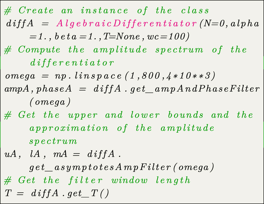
Design of an algebraic differentiator from desired frequency-domain properties.
The amplitude spectrum, the approximation, the bounds, and the phase spectrum are given in Figure 3. Note that for this parametrisation the amplitude spectrum has infinitely many zeros. Thus, its lower bound is equal to zero (see also [22]).
![Figure 3:
Amplitude and phase spectra of the differentiator from Code snippet 2. The approximation (2) and the upper bound from [22, 25] are also given.](/document/doi/10.1515/auto-2023-0035/asset/graphic/j_auto-2023-0035_fig_003.jpg)
Amplitude and phase spectra of the differentiator from Code snippet 2. The approximation (2) and the upper bound from [22, 25] are also given.
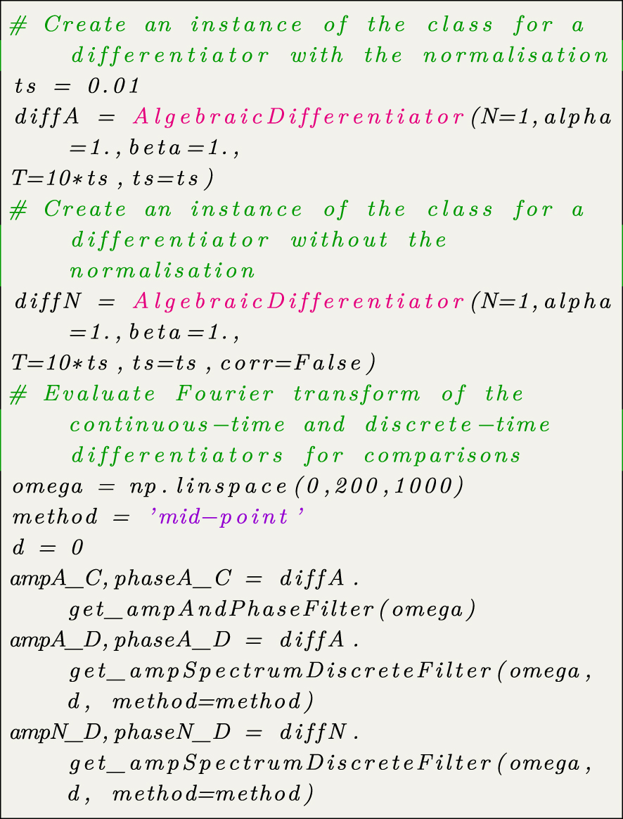
Example 3
(Differentiators with and without delay). As discussed in Section 3, algebraic differentiators can also be parametrised such that the estimated derivative is delay-free. This is done in Code snippet 3 for a differentiator with N = 1 and α = β = 1. Its amplitude spectrum is also computed. For a comparison a differentiator with delay but the same parameters α, β, and N is also considered.
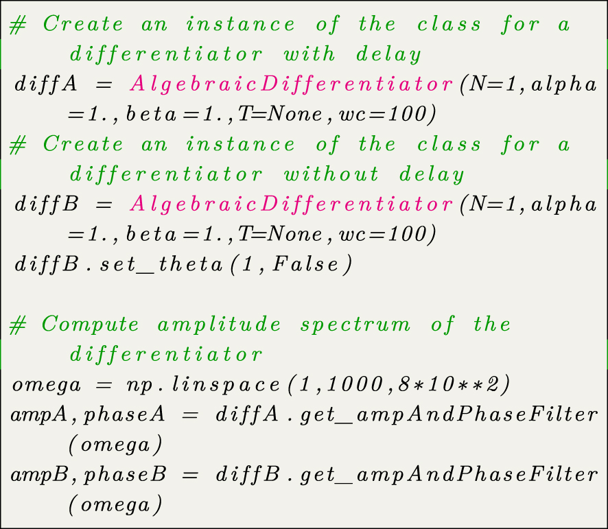
Comparison of amplitude spectra for differentiators with and without delay.
Figure 4 shows the amplitude spectra of both differentiators from the latter example. The delay-free differentiator shows a significant overshoot. Thus, the resulting estimated derivative might not be usable. The decrease in the estimation quality of these differentiators has been remarked in [31]. The overshoots in the amplitude spectra of delay-free differentiators have first been observed in [23].
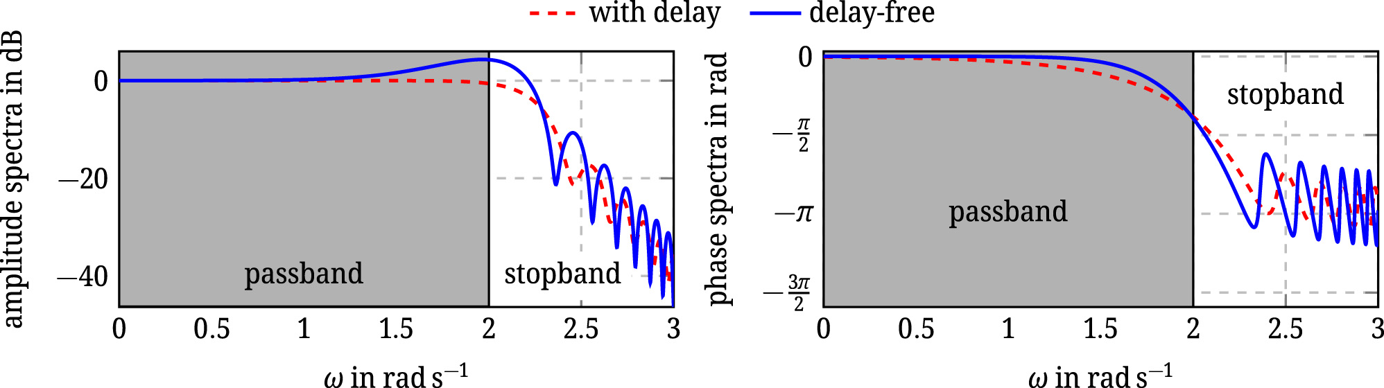
Amplitude and phase spectra of the differentiators with and without delay from Code snippet 3.
It has been observed in [21, 22] that the Fourier transform
where Γ denotes the Gamma Function and
Example 4
(Exact annihilation of frequencies). Assume that the signal the derivative of which has to be estimated is corrupted by a harmonic signal of known frequency ω
0. Choosing the window length T such that ω
0
T = 2j
k
, with j
k
the kth zero of the Bessel function of the first kind and order α + 1/2 yields
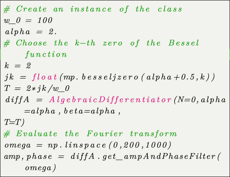
Parametrisation of a differentiator to annihilate a known frequency.
Figure 5 shows the amplitude and phase spectra of this differentiator and confirms the exact annihilation of the disturbing harmonic with frequency ω 0. However, choosing an appropriate zero and a numerical value for α remain as the degrees of freedom for every specific application. The works [21, 22, 29, 30, 33] have proposed an approach where these parameters are chosen such that a satisfying compromise between disturbance rejection and tolerable window length can be achieved. The size T of the window lengths is a crucial parameter since it influences the estimation delay, the computational burden, and the memory requirements of the implemented differentiators. Available hardware may imply constraints on the latter properties.
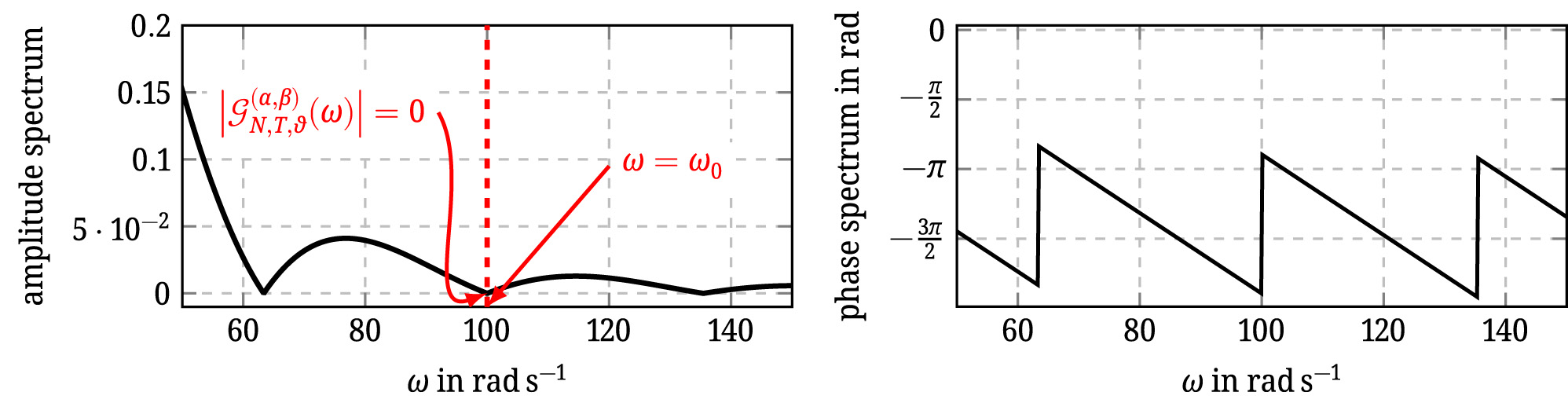
Amplitude and phase spectrum of the differentiator from Code snippet 4 for the annihilation of a harmonic disturbance with angular frequency ω 0.
4.3 Discrete-time implementation
In most applications, the measured signal is available at discrete time instants only and the integral (1) must be approximated by an appropriate quadrature method. Thus, the estimated derivatives are outputs of digital FIR filters.
From the Nyquist–Shannon sampling theorem, it follows that when discretising a continuous-time filter, the gain at the Nyquist frequency must be sufficiently small to keep aliasing effects low. As proposed in [22], a possibility to avoid these effects is to specify the weakest relative attenuation
of an algebraic differentiator
Example 5
(Specifying the relative attenuation k N,min). To achieve at least a desired relative attenuation of k N,min for a given cutoff frequency ω c, the parameters α and β have to be chosen such that
A differentiator is designed in Code snippet 5 for the approximation of a first order derivative with the cutoff frequency equal to 90 rad s−1 and a relative attenuation equal to 10−3 = −30 dB. The considered sampling period is equal to 10 ms, the parameters α and β are chosen equal, and N = 0.
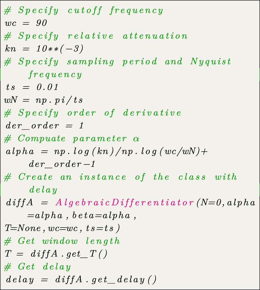
Design of a differentiator with a specified relative attenuation.
The resulting differentiator has a filter window length equal to 100 ms, i.e., 10 sampling periods. The parameters α and β are equal to 5.53. The estimation delay is equal to 5 sampling periods.
In the following, it is assumed that the window length T is an integral multiple of the sampling period, i.e., T = n
s
t
s, and equidistant sampling is considered for simplicity. The abbreviation y
k
= y(kt
s),
of (1) can be achieved. Therein, θ, L, and w
i
depend on the numerical integration method used as discussed in [22, 26, 28]. For example, the mid-point rule yields
Example 6
(Effect of the normalisation factor). Per default, the toolbox implements the normalisation presented in (3). The code in Code snippet 6 demonstrates the effects of the normalisation by comparing the amplitude spectra of two differentiators: The first one is discretised with the normalisation and the second is without.
Discretisation of differentiators with and without normalisation.
Figure 6 shows the spectra of two continuous-time differentiators discretised with and without the normalisation factor. It can be seen that the DC component is only preserved when the normalisation is used.
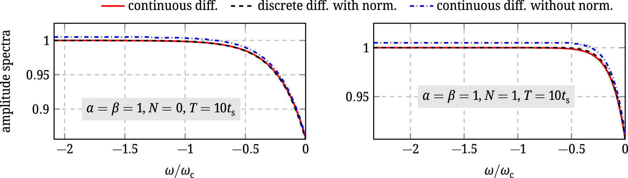
Amplitude of two continuous-time differentiators compared to those of discretised ones with and without normalisation.
Algebraic differentiators and their tuning guidelines have been discussed in the continuous-time domain. Thus, the discretised ones have to preserve the specified properties. Since most tuning guidelines discussed here rely on the frequency-domain interpretation of the differentiators, the analyses of the discretisation effects can be performed by comparing the Fourier transform of the continuous and discrete differentiators. This can be done using the cost function
introduced in [22] (see also [26, 28]), where Ω has to be chosen according to the frequency interval of interest. In the latter cost function,
The cost function
Example 7
(Discretisation error). The cost function (4) is computed in Code snippet 7 for a differentiator with the parameters α = β = 7, N = 0, and T = 20t s.
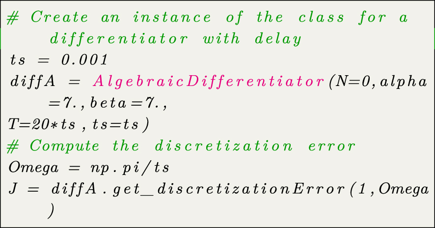
Evaluation of the discretisation error.
The resulting cost
4.4 Estimation of derivatives using AlgDiff
Example 8 demonstrates the numerical differentiation of a given signal using the implemented functions and a differentiator with desired frequency-domain properties.
Example 8
(Numerical differentiation). An algebraic differentiator with the cutoff frequency ω
c = 20 rad s−1 and a desired relative attenuation k
N, min = 10−3 shall be designed for the estimation of the first order derivative of a signal sampled with a sampling period equal to 20 ms. As in Example 2, the choice N = 0 and α = β is made to increase the robustness with respect to disturbances. The resulting differentiator has the parameters α = β = 3.35 and a window length equal to 14t
s. The estimation delay corresponds to 7t
s. The cost function
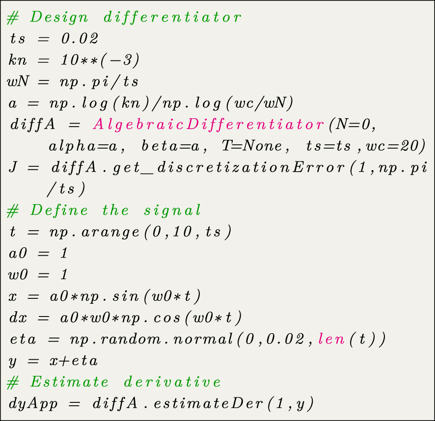
Approximation of a derivative of a given signal using a differentiator designed with desired frequency-domain properties.
The estimation results are shown in Figure 7 and compared to the results of a simple forward difference method. For a comparison with more advanced methods the reader is referred to [25, 34, 35]. This example shows the advantages of algebraic differentiators and their systematic tuning guidelines. Furthermore, it highlights the user friendliness of the toolbox AlgDiff.
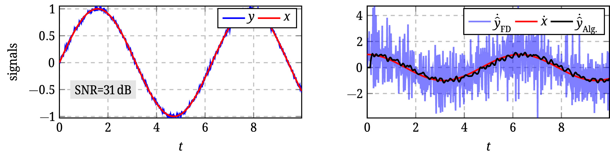
Estimation of the first order derivative
5 Conclusions
This contribution discusses algebraic differentiators and the use of the toolbox AlgDiff. Properties of the differentiators are recalled and the use of the functions implemented in AlgDiff was shown. The design of differentiators with desired frequency-domain properties and the analysis of discretisation issues are addressed with AlgDiff and the results are discussed and illustrated. It is shown that with few lines of code, efficient differentiators can be designed and used for the numerical differentiation of signals. Further works where the systematic tuning of the differentiators are discussed in detail are [21, 22, 25, 26, 28, 30, 33, 36], for example. An extensive list of applications and more examples for the tuning of the differentiators are provided in [26].
About the authors

Amine Othmane received a bachelor’s degree in Mechatronik from Saarland University and a master’s degree in Engineering Cybernetics from the University of Stuttgart. He was a visiting student at the University of Alberta in Edmonton, Canada, and the Norwegian University of Science and Technology in Trondheim, Norway. He received his doctoral degree in 2022 from Saarland University and Université Paris-Saclay, France, in the context of a joint international doctoral supervision (“cotutelle”). Since 2023 he has been working with Prof. Kathrin Flaßkamp (Systems Modeling and Simulation, Saarland University) on combining physics-based and data-based approaches for wind energy systems. He received the best presentation award at the 57. Regelungstechnisches Kolloquium in Boppard. His main research topics are numerical differentiation, parameter estimation, fault diagnosis, model-free control, numerical methods, and physics-based AI methods.

Joachim Rudolph received the doctorate degree from Université Paris XI, Orsay, France, in 1991, and the Dr.-Ing. habil. degree from Technische Universität Dresden, Germany, in 2003. Since 2009, he has been the Head of the Chair of Systems Theory and Control Engineering at Saarland University, Saarbrücken, Germany. His current research interests include controller and observer design for non-linear and infinite dimensional systems, algebraic systems theory, and the solution of demanding practical control problems.
-
Author contributions: All the authors have accepted responsibility for the entire content of this submitted manuscript and approved submission.
-
Research funding: None declared.
-
Conflict of interest statement: The authors declare no conflicts of interest regarding this article.
Appendix A: Jacobi polynomials
The Jacobi polynomial
where
Appendix B: Kernel of algebraic differentiators
The kernel
with θ
T
(t) = 1 − 2t/T and
Appendix C: Impulse and step responses
The impulse and step responses of an algebraic differentiator
respectively, with
Appendix D: Fourier transform
G
N
,
T
,
ϑ
(
α
,
β
)
Closed forms of the Fourier transform
with
where
Appendix E: Cutoff frequency ω c
Let μ = 1 + min{α, β},
where
References
[1] C.-K. Chen and J.-H. Lee, “Design of high-order digital differentiators using L1 error criteria,” IEEE Trans. Circuits Syst. II. Analog Digit. Signal Process., vol. 42, no. 4, pp. 287–291, 1995. https://doi.org/10.1109/82.378044.Search in Google Scholar
[2] C. M. Rader and L. B. Jackson, “Approximating noncausal IIR digital filters having arbitrary poles, including new Hilbert transformer designs, via forward/backward block recursion,” IEEE Trans. Circuits Syst. I Regul. Pap., vol. 53, no. 12, pp. 2779–2787, 2006. https://doi.org/10.1109/TCSI.2006.883877.Search in Google Scholar
[3] D. A. Murio, The Mollification Method and the Numerical Solution of Ill-Posed Problems, New York, Santa Barbara, London, Sydney, Toronto, John Wiley & Sons, 2011.Search in Google Scholar
[4] J. Cullum, “Numerical differentiation and regularization,” SIAM J. Numer. Anal., vol. 8, no. 2, pp. 254–265, 1971. https://doi.org/10.1137/0708026.Search in Google Scholar
[5] A. Levant, “Robust exact differentiation via sliding mode technique,” Automatica, vol. 34, no. 3, pp. 379–384, 1998. https://doi.org/10.1016/S0005-1098(97)00209-4.Search in Google Scholar
[6] A. M. Dabroom and H. K. Khalil, “Numerical differentiation using high-gain observers,” in Proc. of the 36th IEEE Conf. on Decision and Control, vol. 5, San Diego, CA, USA, IEEE, 1997, pp. 4790–4795.10.1109/CDC.1997.649776Search in Google Scholar
[7] A. M. Dabroom and H. K. Khalil, “Discrete-time implementation of high-gain observers for numerical differentiation,” Int. J. Control, vol. 72, no. 17, pp. 1523–1537, 1999. https://doi.org/10.1080/002071799220029.Search in Google Scholar
[8] A. Levant, “Higher-order sliding modes, differentiation and output-feedback control,” Int. J. Control, vol. 76, nos. 9–10, pp. 924–941, 2003. https://doi.org/10.1080/0020717031000099029.Search in Google Scholar
[9] Y. Chitour, “Time-varying high-gain observers for numerical differentiation,” IEEE Trans. Automat. Contr., vol. 47, no. 9, pp. 1565–1569, 2002. https://doi.org/10.1109/TAC.2002.802740.Search in Google Scholar
[10] A. Savitzky and M. J. E. Golay, “Smoothing and differentiation of data by simplified least squares procedures,” Anal. Chem., vol. 36, no. 8, pp. 1627–1639, 1964. https://doi.org/10.1021/ac60214a047.Search in Google Scholar
[11] H. Madden, “Comments on the Savitzky–Golay convolution method for least-squares fit smoothing and differentiation of digital data,” Anal. Chem., vol. 50, no. 9, pp. 1383–1386, 1978. https://doi.org/10.1021/ac50031a048.Search in Google Scholar
[12] E. Diekema and T. H. Koornwinder, “Differentiation by integration using orthogonal polynomials, a survey,” J. Approx. Theor., vol. 164, no. 5, pp. 637–667, 2012. https://doi.org/10.1016/j.jat.2012.01.003.Search in Google Scholar
[13] N. Cioranescu, “La généralisation de la première formule de la moyenne,” Enseign. Math., vol. 37, pp. 292–302, 1938.Search in Google Scholar
[14] C. Lanczos, Applied Analysis, Englewood Cliffs, Prentice Hall, Inc., 1956.Search in Google Scholar
[15] M. Mboup, C. Join, and M. Fliess, “A revised look at numerical differentiation with an application to nonlinear feedback control,” in Proc. of the 15th Mediterranean Conf. on Control and Automation, Athen, Greece, IEEE, 2007.10.1109/MED.2007.4433728Search in Google Scholar
[16] M. Mboup, C. Join, and M. Fliess, “Numerical differentiation with annihilators in noisy environment,” Numer. Algorithm., vol. 50, no. 4, pp. 439–467, 2009. https://doi.org/10.1007/s11075-008-9236-1.Search in Google Scholar
[17] J. Reger and J. Jouffroy, “On algebraic time-derivative estimation and deadbeat state reconstruction,” in Proc. of the 48h IEEE Conf. on Decision and Control Held jointly with 2009 28th Chinese Control Conf, Shanghai, China, IEEE, 2009, pp. 1740–1745.10.1109/CDC.2009.5400719Search in Google Scholar
[18] J. Reger and J. Jouffroy, “Algebraische Ableitungsschätzung im Kontext der Rekonstruierbarkeit (Algebraic time-derivative estimation in the context of reconstructibility),” Automatisierungstechnik, vol. 56, no. 6, pp. 324–331, 2008. https://doi.org/10.1524/auto.2008.0711.Search in Google Scholar
[19] D. Y. Liu, O. Gibaru, and W. Perruquetti, “Convergence rate of the causal Jacobi derivative estimator,” in Curves and Surfaces, J.-D. Boissonnat, P. Chenin, A. Cohen, et al.., Eds., Berlin, Heidelberg, Springer, 2010, pp. 445–455.10.1007/978-3-642-27413-8_28Search in Google Scholar
[20] D. Y. Liu, O. Gibaru, and W. Perruquetti, “Error analysis of Jacobi derivative estimators for noisy signals,” Numer. Algorithm., vol. 58, no. 1, pp. 53–83, 2011. https://doi.org/10.1007/s11075-011-9447-8.Search in Google Scholar
[21] L. Kiltz and J. Rudolph, “Parametrization of algebraic numerical differentiators to achieve desired filter characteristics,” in Proc. of the 52nd IEEE Conf. on Decision and Control, Florence, Italy, IEEE, 2013, pp. 7010–7015.10.1109/CDC.2013.6761000Search in Google Scholar
[22] L. Kiltz, “Algebraische Ableitungsschätzer in Theorie und Anwendung,” Doctoral dissertation, Saarland University, Germany, 2017.Search in Google Scholar
[23] M. Mboup and S. Riachy, “A frequency domain interpretation of the algebraic differentiators,” IFAC Proc. Vol., vol. 47, no. 3, pp. 9147–9151, 2014. https://doi.org/10.3182/20140824-6-za-1003.02132.Search in Google Scholar
[24] M. Mboup and S. Riachy, “Frequency-domain analysis and tuning of the algebraic differentiators,” Int. J. Control, vol. 91, no. 9, pp. 2073–2081, 2018. https://doi.org/10.1080/00207179.2017.1421776.Search in Google Scholar
[25] A. Othmane, J. Rudolph, and H. Mounier, “Systematic comparison of numerical differentiators and an application to model-free control,” Eur. J. Control, vol. 62, pp. 113–119, 2021. https://doi.org/10.1016/j.ejcon.2021.06.020.Search in Google Scholar
[26] A. Othmane, L. Kiltz, and J. Rudolph, “Survey on algebraic numerical differentiation: historical developments, parametrization, examples, and applications,” Int. J. Syst. Sci., vol. 53, no. 9, pp. 1848–1887, 2022. https://doi.org/10.1080/00207721.2022.2025948.Search in Google Scholar
[27] A. Othmane, AlgDiff: A Python Package with MATLAB Coupling Implementing All Necessary Tools for the Design, Analysis, and Discretization of Algebraic Differentiators, Version 1.1.1, 2023. Available at: https://github.com/aothmane-control/Algebraic-differentiators.Search in Google Scholar
[28] A. Othmane, “Contributions to numerical differentiation using orthogonal polynomials and its application to fault detection and parameter identification,” Doctoral dissertation, Université Paris-Saclay, Germany, Saarland University, France, 2022, p. 2022.Search in Google Scholar
[29] L. Kiltz, M. Mboup, and J. Rudolph, “Fault diagnosis on a magnetically supported plate,” in Proc. of the 1st International Conf. on Systems and Computer Science, Lille, France, IEEE, 2012.10.1109/IConSCS.2012.6502453Search in Google Scholar
[30] L. Kiltz, C. Join, M. Mboup, and J. Rudolph, “Fault-tolerant control based on algebraic derivative estimation applied on a magnetically supported plate,” Control Eng. Pract., vol. 26, pp. 107–115, 2014. https://doi.org/10.1016/j.conengprac.2014.01.009.Search in Google Scholar
[31] M. Mboup, “Parameter estimation for signals described by differential equations,” Appl. Anal., vol. 88, no. 1, pp. 29–52, 2009. https://doi.org/10.1080/00036810802555441.Search in Google Scholar
[32] M. Abramowitz and I. A. Stegun, Eds. Handbook of Mathematical Functions with Formulas, Graphs, and Mathematical Tables, New York, Dover, 1965.10.1063/1.3047921Search in Google Scholar
[33] L. Kiltz, M. Janocha, and J. Rudolph, “Algebraic estimation of impact times: juggling a ball with a magnetically levitated plate,” in Proc. of the 2nd International Conf. on Systems and Computer Science, France, Villeneuve d’Ascq, 2013, pp. 145–149.10.1109/IcConSCS.2013.6632038Search in Google Scholar
[34] L. Sidhom, “Sur les différentiateurs en temps réel: algorithmes et applications,” Doctoral dissertation, INSA de Lyon, France, 2011.Search in Google Scholar
[35] D. Y. Liu, “Analyse d’erreurs d’estimateurs des dérivées de signaux bruités et applications,” Doctoral dissertation, Université des Sciences et Technologies de Lille – Lille 1, France, 2011.Search in Google Scholar
[36] P. M. Scherer, A. Othmane, and J. Rudolph, “Combining model-based and model-free approaches for the control of an electro-hydraulic system,” Control Eng. Pract., vol. 133, p. 105453, 2023. https://doi.org/10.1016/j.conengprac.2023.105453.Search in Google Scholar
© 2023 Walter de Gruyter GmbH, Berlin/Boston
Articles in the same Issue
- Frontmatter
- Drei Beiträge vom Ausschuss FA 2.13
- Editorial
- Ausgewählte Beiträge der GMA-Fachausschüsse 2.13 und 2.14
- Applications
- Modeling and identification of the hydration process in a CaO/Ca(OH) 2 -based heat storage system
- Anwendungen
- Indirekte Schätzung der Magnettemperatur einer Permanentmagnet-Synchronmaschine
- Tools
- AlgDiff: an open source toolbox for the design, analysis and discretisation of algebraic differentiators
- Drei Beiträge vom Ausschuss FA 2.14
- Survey
- Control of distributed-parameter systems using normal forms: an introduction
- Methoden
- Einbettungsbeobachter für polynomiale Systeme
- Anwendungen
- Flachheitsbasierte Trajektorienfolgeregelung eines pneumatischen Roboters
- Applications
- Semi-automatic assessment of lack of control code documentation in automated production systems
- Survey
- Towards asset administration shell-based continuous engineering in process industries
- Methods
- A workflow towards a strongly typed AutomationML API
- Persönliches
- Prof. Dr.-Ing. Ulrich Epple zum 70. Geburtstag