The Liability Insurance Consumption Spiral: Evidence from Chinese Cities

Douglas Bujakowski

doi:10.1515/apjri-2025-0008

Article

The Liability Insurance Consumption Spiral: Evidence from Chinese Cities

Douglas Bujakowski

Published/Copyright: November 5, 2025

Published by

Become an author with De Gruyter Brill

Submit Manuscript Author Information Explore this Subject

From the journal Asia-Pacific Journal of Risk and Insurance

Abstract

Liability insurance is a vital source of financial protection and risk management for individuals and organizations. However, its widespread adoption carries certain unintended consequences, including the amplification of liability risks for uninsured and underinsured populations. This may result in a liability insurance consumption spiral, where purchases by some incentivize others to follow suit. The current study provides the first empirical tests of the consumption spiral hypothesis. Using data from 280 Chinese cities over an eight-year period (2011–2018), we find evidence that liability insurance purchases influence those in nearby geographic units and subsequent time periods. These knock-on effects are substantial and support the notion that purchase decisions are positively correlated. Additionally, our results reveal a key externality of liability insurance markets and the ways in which consumption diffuses across space and time.

Keywords: spatial model; insurance consumption; spillover effect; China

JEL Classification: G01; G22; E22

Corresponding author: Douglas Bujakowski, Associate Professor, Bowling Green State University, 1001 E Wooster St, Bowling Green, OH 43403, USA, E-mail: dbujak@bgsu.edu

Research ethics: Not applicable.
Informed consent: Not applicable.
Author contributions: The author has accepted responsibility for the entire content of this manuscript and approved its submission.
Use of Large Language Models, AI and Machine Learning Tools: None declared.
Conflict of interest: The author states no conflict of interest.
Research funding: None declared.
Data availability: The data used in this study are publicly available but require a purchase for access. Specifically, the data were obtained from the China Statistical Yearbooks Database (CSYD), maintained by the National Bureau of Statistics of China. This database includes statistical yearbooks focusing on various regions and industries, including the China Insurance Yearbook and the China City Statistical Yearbooks, which were used to construct the variables for this study. Interested researchers can access the CSYD via National Bureau of Statistics of China or through authorized vendors, subject to the database’s purchase and licensing terms.

Appendix

See Tables 1A–11A and Figure 1A.

Table 1A:

Insurance density model estimates – spatial errors.

	Model 1			Model 2			Model 3			Model 4
	Est.	S.E.		Est.	S.E.		Est.	S.E.		Est.	S.E.
Spatial lag (ρ)				0.335	0.027	***				0.415	0.055	***
Spatial error (φ)							0.059	0.006	***	−0.023	0.016
GDP	0.166	0.070	**	0.174	0.067	**	0.265	0.075	***	0.151	0.066	**
Disp. Income	−0.363	0.104	***	−0.335	0.100	***	−0.374	0.107	***	−0.305	0.097	***
Agriculture	−0.253	0.051	***	−0.191	0.050	***	−0.196	0.054	***	−0.188	0.048	***
Manufacturing	0.008	0.074		−0.028	0.072		−0.042	0.075		−0.021	0.070
Loans	−0.040	0.039		−0.020	0.037		−0.027	0.039		−0.011	0.037
HHI	0.214	0.021	***	0.195	0.021	***	0.202	0.021	***	0.194	0.021	***
Edu (Higher Ed)	0.000	0.023		−0.002	0.022		−0.003	0.023		0.000	0.022
Edu (Vocational)	−0.012	0.019		−0.022	0.018		−0.025	0.019		−0.019	0.018
Edu Expend.	0.135	0.048	***	0.125	0.046	***	0.150	0.049	***	0.114	0.045	**
Unemployment	−0.015	0.021		−0.018	0.020		−0.025	0.021		−0.016	0.020
Internet	0.031	0.025		0.014	0.025		0.008	0.026		0.012	0.024
Cell phones	−0.007	0.037		0.018	0.036		0.021	0.038		0.013	0.035
Tourism	0.014	0.006	**	0.010	0.006	*	0.010	0.006	*	0.010	0.006	*
City FE	Yes			Yes			Yes			Yes
Year FE	Yes			Yes			Yes			Yes
Observations	2,240			2,240			2,240			2,240
Log-likelihood	747.2			808.4			794.3			808.7

The table shows estimates of Equation (3) using liability insurance premium density as the dependent variable. Liability insurance premium density is defined as the natural log of real city-level liability insurance premiums written per capita. The sample period is 2011–2018. Models 1–3 are limiting cases of Model 4 in that ρ, φ, or both are constrained to be zero. Model 4 is unconstrained. All models include a constant term, city and year fixed effects, and economic and demographic variables. See Table 1 for variable definitions. ***, **, and * denote significance at the 1 %, 5 %, and 10 % levels, respectively.

Table 2A:

Insurance penetration model estimates – spatial errors.

	Model 1			Model 2			Model 3			Model 4
	Est.	S.E.		Est.	S.E.		Est.	S.E.		Est.	S.E.
Spatial lag (ρ)				0.358	0.025	***				0.434	0.055	***
Spatial error (φ)							0.070	0.005	***	−0.022	0.017
Disp. Income	−0.713	0.103	***	−0.560	0.098	***	−0.625	0.107	***	−0.528	0.097	***
Agriculture	−0.114	0.052	**	−0.053	0.049		−0.044	0.053		−0.056	0.048
Manufacturing	−0.278	0.073	***	−0.251	0.069	***	−0.277	0.073	***	−0.239	0.068	***
Loans	0.167	0.036	***	0.117	0.035	***	0.130	0.037	***	0.116	0.034	***
HHI	0.194	0.022	***	0.187	0.021	***	0.189	0.021	***	0.186	0.021	***
Population	−0.013	0.188		0.146	0.179		0.247	0.189		0.120	0.175
Edu (Higher Ed)	0.009	0.024		0.018	0.023		0.009	0.023		0.021	0.023
Edu (Vocational)	−0.034	0.020	*	−0.038	0.019	**	−0.044	0.019	**	−0.035	0.018	*
Edu Expend.	0.379	0.045	***	0.331	0.043	***	0.342	0.046	***	0.322	0.043	***
Unemployment	0.018	0.021		−0.003	0.020		−0.005	0.021		−0.003	0.020
Internet	−0.037	0.026		−0.024	0.024		−0.029	0.027		−0.023	0.024
Cell phones	−0.097	0.039	**	−0.066	0.037	*	−0.036	0.039		−0.074	0.036	**
Tourism	0.012	0.006	*	0.010	0.006	*	0.010	0.006		0.010	0.006	*
City FE	Yes			Yes			Yes			Yes
Year FE	Yes			Yes			Yes			Yes
Observations	2,240			2,240			2,240			2,240
Log-likelihood	677.5			761.2			749.1			761.3

The table shows estimates of Equation (3) using liability insurance premium penetration as the dependent variable. Liability insurance premium penetration is defined as the natural log of city-level liability insurance premiums written per GDP. The sample period is 2011–2018. Models 1–3 are limiting cases of Model 4 in that ρ, φ, or both are constrained to be zero. Model 4 is unconstrained. All models include a constant term, city and year fixed effects, and economic and demographic variables. See Table 1 for variable definitions. ***, **, and * denote significance at the 1 %, 5 %, and 10 % levels, respectively.

Table 3A:

Likelihood ratio tests – spatial errors.

Nested model	General model	χ ²	p-Value
Panel A: Insurance density
Model 1	Model 2	122.5	<0.001
Model 1	Model 3	94.2	<0.001
Model 1	Model 4	123.0	<0.001
Model 2	Model 4	0.6	0.439
Model 3	Model 4	28.8	<0.001
Panel B: Insurance penetration
Model 1	Model 2	167.4	<0.001
Model 1	Model 3	143.2	<0.001
Model 1	Model 4	167.6	<0.001
Model 2	Model 4	0.2	0.655
Model 3	Model 4	24.4	<0.001

The table shows likelihood ratio test results from the analysis in Tables 1A and 2A. Panels A and B of the table make use of the log likelihood values reported in Tables 1A and 2A, respectively.

Table 4A:

Insurance density model estimates – coastal provinces.

	Model 1			Model 2			Model 3			Model 4
	Est.	S.E.		Est.	S.E.		Est.	S.E.		Est.	S.E.
Spatial lag (ρ)				0.335	0.041	***				0.209	0.046	***
Time lag (λ)							0.466	0.035	***	0.437	0.035	***
GDP	−0.096	0.120		−0.058	0.118		0.121	0.128		0.102	0.126
Disp. Income	−0.623	0.210	***	−0.616	0.204	***	−0.578	0.224	***	−0.575	0.220	***
Agriculture	−0.392	0.092	***	−0.291	0.091	***	−0.286	0.097	***	−0.232	0.097	**
Manufacturing	−0.314	0.135	**	−0.291	0.132	**	−0.432	0.144	***	−0.414	0.141	***
Loans	−0.024	0.072		0.006	0.070		−0.015	0.079		−0.003	0.078
HHI	0.302	0.032	***	0.275	0.031	***	0.230	0.033	***	0.219	0.033	***
Edu (Higher Ed)	0.067	0.051		0.063	0.050		0.042	0.054		0.044	0.053
Edu (Vocational)	0.006	0.037		−0.023	0.036		−0.001	0.039		−0.024	0.039
Edu Expend.	−0.090	0.081		−0.068	0.079		0.040	0.086		0.035	0.085
Unemployment	0.053	0.036		0.039	0.035		0.069	0.038	*	0.056	0.037
Internet	0.166	0.048	***	0.124	0.047	***	0.136	0.052	***	0.108	0.051	**
Cell phones	−0.109	0.067		−0.081	0.066		−0.054	0.073		−0.035	0.072
Tourism	−0.049	0.016	***	−0.040	0.015	***	−0.018	0.017		−0.016	0.017
City FE	Yes			Yes			Yes			Yes
Year FE	Yes			Yes			Yes			Yes
Observations	864			864			756			756
Log-likelihood	321.5			343.5			331.0			340.8

The table shows estimates of Equation (1) using liability insurance premium density as the dependent variable. Liability insurance premium density is defined as the natural log of real city-level liability insurance premiums written per capita. The sample includes cities in coastal provinces: Beijing, Guangdong, Guangxi, Fujian, Hainan, Hebei, Jiangsu, Liaoning, Shandong, Shanghai, Tianjin, and Zhejiang. The sample period is 2011–2018. Models 1–3 are limiting cases of Model 4 in that ρ, λ, or both are constrained to be zero. Model 4 is unconstrained. All models include a constant term, city and year fixed effects, and economic and demographic variables. See Table 1 for variable definitions. ***, **, and * denote significance at the 1 %, 5 %, and 10 % levels, respectively.

Table 5A:

Insurance density model estimates – inland provinces.

	Model 1			Model 2			Model 3			Model 4
	Est.	S.E.		Est.	S.E.		Est.	S.E.		Est.	S.E.
Spatial lag (ρ)				0.266	0.033	***				0.121	0.034	***
Time lag (λ)							0.800	0.025	***	0.771	0.025	***
GDP	0.433	0.087	***	0.396	0.084	***	0.159	0.080	**	0.150	0.079	*
Disp. Income	−0.284	0.121	**	−0.259	0.118	**	−0.125	0.120		−0.135	0.119
Agriculture	−0.173	0.061	***	−0.138	0.060	**	0.010	0.056		0.019	0.055
Manufacturing	0.057	0.088		0.021	0.086		0.010	0.080		−0.002	0.079
Loans	−0.060	0.047		−0.059	0.046		0.043	0.044		0.039	0.043
HHI	0.108	0.028	***	0.100	0.027	***	0.070	0.026	***	0.070	0.025	***
Edu (Higher Ed)	−0.008	0.025		−0.007	0.025		0.011	0.024		0.008	0.024
Edu (Vocational)	−0.036	0.022	*	−0.039	0.021	*	0.004	0.021		−0.001	0.021
Edu Expend.	0.285	0.060	***	0.255	0.058	***	−0.009	0.056		−0.010	0.056
Unemployment	−0.060	0.025	**	−0.063	0.024	***	−0.020	0.023		−0.023	0.023
Internet	−0.019	0.030		−0.035	0.030		0.007	0.028		−0.001	0.028
Cell phones	0.089	0.045	**	0.092	0.044	**	−0.034	0.043		−0.031	0.042
Tourism	0.031	0.007	***	0.025	0.007	***	0.019	0.006	***	0.017	0.006	***
City FE	Yes			Yes			Yes			Yes
Year FE	Yes			Yes			Yes			Yes
Observations	1,376			1,376			1,204			1,204
Log-likelihood	496.8			527.8			698.7			708.1

The table shows estimates of Equation (1) using liability insurance premium density as the dependent variable. Liability insurance premium density is defined as the natural log of real city-level liability insurance premiums written per capita. The sample includes cities in inland provinces: Anhui, Chongqing, Gansu, Heilongjiang, Henan, Hubei, Hunan, Inner Mongolia, Jiangxi, Jilin, Qinghai, Shaanxi, Shanxi, Sichuan, Xinjiang, and Yunnan. The sample period is 2011–2018. Models 1–3 are limiting cases of Model 4 in that ρ, λ, or both are constrained to be zero. Model 4 is unconstrained. All models include a constant term, city and year fixed effects, and economic and demographic variables. See Table 1 for variable definitions. ***, **, and * denote significance at the 1 %, 5 %, and 10 % levels, respectively.

Table 6A:

Insurance penetration model estimates – coastal provinces.

	Model 1			Model 2			Model 3			Model 4
	Est.	S.E.		Est.	S.E.		Est.	S.E.		Est.	S.E.
Spatial lag (ρ)				0.335	0.040	***				0.188	0.044	***
Time lag (λ)							0.484	0.033	***	0.457	0.033	***
Disp. Income	−0.947	0.216	***	−0.854	0.211	***	−0.652	0.225	***	−0.617	0.222	***
Agriculture	−0.181	0.095	*	−0.105	0.093		−0.182	0.097	*	−0.138	0.096
Manufacturing	−0.654	0.136	***	−0.587	0.133	***	−0.602	0.142	***	−0.582	0.140	***
Loans	0.336	0.063	***	0.254	0.062	***	0.188	0.066	***	0.149	0.066	**
HHI	0.293	0.034	***	0.275	0.033	***	0.226	0.034	***	0.221	0.034	***
Population	−0.400	0.418		0.043	0.410		0.475	0.428		0.623	0.424
Edu (Higher Ed)	0.076	0.054		0.081	0.052		0.050	0.055		0.055	0.054
Edu (Vocational)	0.024	0.038		−0.016	0.037		−0.003	0.040		−0.027	0.039
Edu Expend.	0.143	0.081	*	0.127	0.079		0.186	0.082	**	0.165	0.081	**
Unemployment	0.137	0.037	***	0.091	0.036	**	0.095	0.038	**	0.070	0.038	*
Internet	0.062	0.050		0.063	0.049		0.129	0.052	**	0.119	0.052	**
Cell phones	−0.196	0.070	***	−0.164	0.068	**	−0.098	0.074		−0.081	0.073
Tourism	−0.044	0.017	***	−0.035	0.016	**	−0.020	0.017		−0.017	0.017
City FE	Yes			Yes			Yes			Yes
Year FE	Yes			Yes			Yes			Yes
Observations	864			864			756			756
Log-likelihood	282.4			307.5			317.4			326.4

The table shows estimates of Equation (1) using liability insurance premium penetration as the dependent variable. Liability insurance premium penetration is defined as the natural log of city-level liability insurance premiums written per GDP. The sample includes cities in coastal provinces: Beijing, Guangdong, Guangxi, Fujian, Hainan, Hebei, Jiangsu, Liaoning, Shandong, Shanghai, Tianjin, and Zhejiang. The sample period is 2011–2018. Models 1–3 are limiting cases of Model 4 in that ρ, λ, or both are constrained to be zero. Model 4 is unconstrained. All models include a constant term, city and year fixed effects, and economic and demographic variables. See Table 1 for variable definitions. ***, **, and * denote significance at the 1 %, 5 %, and 10 % levels, respectively.

Table 7A:

Insurance penetration model estimates – inland provinces.

	Model 1			Model 2			Model 3			Model 4
	Est.	S.E.		Est.	S.E.		Est.	S.E.		Est.	S.E.
Spatial lag (ρ)				0.293	0.032	***				0.159	0.033	***
Time lag (λ)							0.802	0.026	***	0.764	0.026	***
Disp. Income	−0.518	0.118	***	−0.432	0.114	***	−0.098	0.121		−0.092	0.120
Agriculture	−0.083	0.060		−0.039	0.058		0.020	0.056		0.036	0.056
Manufacturing	−0.151	0.084	*	−0.136	0.081	*	−0.051	0.078		−0.046	0.077
Loans	0.062	0.044		0.026	0.042		0.116	0.042	***	0.094	0.041	**
HHI	0.083	0.028	***	0.091	0.027	***	0.082	0.026	***	0.085	0.026	***
Population	0.046	0.209		0.153	0.202		−0.142	0.191		−0.086	0.189
Edu (Higher Ed)	0.005	0.026		0.011	0.025		−0.005	0.025		−0.004	0.025
Edu (Vocational)	−0.062	0.022	***	−0.056	0.021	***	0.016	0.022		0.013	0.022
Edu Expend.	0.450	0.055	***	0.418	0.053	***	0.067	0.053		0.070	0.052
Unemployment	−0.052	0.025	**	−0.059	0.024	**	0.005	0.024		−0.002	0.024
Internet	−0.059	0.030	*	−0.061	0.029	**	0.014	0.028		0.009	0.028
Cell phones	0.030	0.046		0.027	0.044		−0.032	0.044		−0.034	0.043
Tourism	0.030	0.007	***	0.024	0.007	***	0.023	0.006	***	0.019	0.006	***
City FE	Yes			Yes			Yes			Yes
Year FE	Yes			Yes			Yes			Yes
Observations	1,376			1,376			1,204			1,204
Log-likelihood	475.7			515.5			657.1			671.1

The table shows estimates of Equation (1) using liability insurance premium penetration as the dependent variable. Liability insurance premium penetration is defined as the natural log of city-level liability insurance premiums written per GDP. The sample includes cities in inland provinces: Anhui, Chongqing, Gansu, Heilongjiang, Henan, Hubei, Hunan, Inner Mongolia, Jiangxi, Jilin, Qinghai, Shaanxi, Shanxi, Sichuan, Xinjiang, and Yunnan. The sample period is 2011–2018. Models 1–3 are limiting cases of Model 4 in that ρ, λ, or both are constrained to be zero. Model 4 is unconstrained. All models include a constant term, city and year fixed effects, and economic and demographic variables. See Table 1 for variable definitions. ***, **, and * denote significance at the 1 %, 5 %, and 10 % levels, respectively.

Table 8A:

Insurance density model estimates – high litigation provinces.

	Model 1			Model 2			Model 3			Model 4
	Est.	S.E.		Est.	S.E.		Est.	S.E.		Est.	S.E.
Spatial lag (ρ)				0.300	0.049	***				0.047	0.054
Time lag (λ)							0.620	0.039	***	0.612	0.040	***
GDP	−0.314	0.182	*	−0.225	0.185		0.211	0.187		0.213	0.187
Disp. Income	0.560	0.216	***	0.495	0.217	**	0.065	0.215		0.053	0.215
Agriculture	−0.291	0.104	***	−0.241	0.105	**	−0.088	0.101		−0.085	0.101
Manufacturing	0.054	0.178		0.082	0.179		−0.337	0.176	*	−0.312	0.175	*
Loans	−0.067	0.076		−0.036	0.077		−0.030	0.077		−0.029	0.078
HHI	0.127	0.042	***	0.126	0.043	***	0.085	0.040	**	0.084	0.040	**
Edu (Higher Ed)	−0.025	0.063		−0.026	0.063		0.003	0.061		−0.002	0.060
Edu (Vocational)	0.070	0.043		0.037	0.044		0.012	0.042		0.007	0.042
Edu expend.	−0.069	0.090		0.008	0.091		0.030	0.089		0.038	0.089
Unemployment	−0.014	0.044		0.012	0.045		−0.075	0.044	*	−0.071	0.044
Internet	0.138	0.054	**	0.097	0.054	*	0.039	0.054		0.033	0.055
Cell phones	0.141	0.077	*	0.116	0.077		−0.005	0.075		−0.005	0.075
Tourism	−0.016	0.014		−0.028	0.014	**	0.016	0.014		0.013	0.014
City FE	Yes			Yes			Yes			Yes
Year FE	Yes			Yes			Yes			Yes
Observations	624			624			546			546
Log-likelihood	256.2			265.4			306.1			307.1

The table shows estimates of Equation (1) using liability insurance premium density as the dependent variable. Liability insurance premium density is defined as the natural log of real city-level liability insurance premiums written per capita. The sample includes cities in high litigation provinces: Anhui, Beijing, Chongqing, Fujian, Guangdong, Hainan, Jiangsu, Ningxia, Shanghai, Tianjin, Xinjiang, and Zhejiang. The sample period is 2011–2018. Models 1–3 are limiting cases of Model 4 in that ρ, λ, or both are constrained to be zero. Model 4 is unconstrained. All models include a constant term, city and year fixed effects, and economic and demographic variables. See Table 1 for variable definitions. ***, **, and * denote significance at the 1 %, 5 %, and 10 % levels, respectively.

Table 9A:

Insurance density model estimates – low litigation provinces.

	Model 1			Model 2			Model 3			Model 4
	Est.	S.E.		Est.	S.E.		Est.	S.E.		Est.	S.E.
Spatial lag (ρ)				0.284	0.039	***				0.153	0.040	***
Time lag (λ)							0.675	0.029	***	0.651	0.029	***
GDP	0.474	0.094	***	0.482	0.092	***	0.277	0.093	***	0.283	0.092	***
Disp. Income	−0.426	0.148	***	−0.456	0.145	***	−0.122	0.157		−0.172	0.155
Agriculture	−0.296	0.073	***	−0.239	0.072	***	−0.182	0.071	**	−0.153	0.071	**
Manufacturing	−0.179	0.108	*	−0.242	0.106	**	−0.167	0.104		−0.197	0.103	*
Loans	0.090	0.066		0.098	0.065		0.170	0.064	***	0.171	0.063	***
HHI	0.188	0.032	***	0.177	0.032	***	0.125	0.031	***	0.125	0.030	***
Edu (Higher Ed)	−0.029	0.030		−0.025	0.029		−0.031	0.030		−0.030	0.030
Edu (Vocational)	−0.060	0.025	**	−0.066	0.025	***	−0.010	0.026		−0.017	0.026
Edu Expend.	0.352	0.073	***	0.308	0.072	***	0.059	0.073		0.047	0.073
Unemployment	−0.057	0.029	**	−0.063	0.028	**	0.000	0.029		−0.007	0.028
Internet	−0.025	0.042		−0.049	0.041		0.027	0.040		0.007	0.040
Cell phones	0.141	0.062	**	0.120	0.060	**	−0.020	0.062		−0.026	0.061
Tourism	0.025	0.008	***	0.017	0.008	**	0.020	0.008	**	0.015	0.008	*
City FE	Yes			Yes			Yes			Yes
Year FE	Yes			Yes			Yes			Yes
Observations	1,056			1,056			924			924
Log-likelihood	346.1			367.3			451.3			460.0

The table shows estimates of Equation (1) using liability insurance premium density as the dependent variable. Liability insurance premium density is defined as the natural log of real city-level liability insurance premiums written per capita. The sample includes cities in low litigation provinces: Guizhou, Heilongjiang, Henan, Hubei, Hunan, Jiangxi, Jilin, Liaoning, Shaanxi, Shanxi, Sichuan, and Qinghai. The sample period is 2011–2018. Models 1–3 are limiting cases of Model 4 in that ρ, λ, or both are constrained to be zero. Model 4 is unconstrained. All models include a constant term, city and year fixed effects, and economic and demographic variables. See Table 1 for variable definitions. ***, **, and * denote significance at the 1 %, 5 %, and 10 % levels, respectively.

Table 10A:

Insurance penetration model estimates – high litigation provinces.

	Model 1			Model 2			Model 3			Model 4
	Est.	S.E.		Est.	S.E.		Est.	S.E.		Est.	S.E.
Spatial lag (ρ)				0.318	0.048	***				0.055	0.053
Time lag (λ)							0.618	0.037	***	0.608	0.038	***
Disp. Income	0.399	0.224	*	0.380	0.220	*	0.001	0.217		0.002	0.217
Agriculture	−0.105	0.105		−0.051	0.104		−0.048	0.097		−0.040	0.097
Manufacturing	−0.323	0.178	*	−0.258	0.175		−0.466	0.171	***	−0.443	0.171	***
Loans	0.142	0.075	*	0.151	0.074	**	0.025	0.075		0.026	0.075
HHI	0.155	0.044	***	0.146	0.044	***	0.097	0.041	**	0.096	0.041	**
Population	−0.032	0.467		0.074	0.459		0.298	0.455		0.303	0.454
Edu (Higher Ed)	0.077	0.064		0.060	0.063		0.000	0.060		−0.004	0.059
Edu (Vocational)	0.074	0.045		0.037	0.045		0.028	0.043		0.022	0.043
Edu Expend.	0.117	0.090		0.163	0.088	*	0.071	0.087		0.077	0.086
Unemployment	0.040	0.046		0.055	0.045		−0.067	0.044		−0.063	0.044
Internet	0.030	0.058		0.016	0.057		0.046	0.058		0.042	0.058
Cell phones	0.005	0.079		−0.023	0.078		−0.021	0.076		−0.024	0.075
Tourism	−0.004	0.015		−0.018	0.015		0.016	0.015		0.013	0.015
City FE	Yes			Yes			Yes			Yes
Year FE	Yes			Yes			Yes			Yes
Observations	624			624			546			546
Log-likelihood	231.2			241.7			299.8			301.1

The table shows estimates of Equation (1) using liability insurance premium penetration as the dependent variable. Liability insurance premium penetration is defined as the natural log of city-level liability insurance premiums written per GDP. The sample includes cities in high litigation provinces: Anhui, Beijing, Chongqing, Fujian, Guangdong, Hainan, Jiangsu, Ningxia, Shanghai, Tianjin, Xinjiang, and Zhejiang. The sample period is 2011–2018. Models 1–3 are limiting cases of Model 4 in that ρ, λ, or both are constrained to be zero. Model 4 is unconstrained. All models include a constant term, city and year fixed effects, and economic and demographic variables. See Table 1 for variable definitions. ***, **, and * denote significance at the 1 %, 5 %, and 10 % levels, respectively.

Table 11A:

Insurance penetration model estimates – low litigation provinces.

	Model 1			Model 2			Model 3			Model 4
	Est.	S.E.		Est.	S.E.		Est.	S.E.		Est.	S.E.
Spatial lag (ρ)				0.318	0.035	***				0.146	0.037	***
Time lag (λ)							0.653	0.030	***	0.619	0.030	***
Disp. Income	−0.688	0.143	***	−0.584	0.137	***	−0.117	0.154		−0.121	0.152
Agriculture	−0.247	0.073	***	−0.165	0.071	**	−0.210	0.072	***	−0.174	0.072	**
Manufacturing	−0.365	0.105	***	−0.395	0.100	***	−0.215	0.102	**	−0.238	0.101	**
Loans	0.263	0.061	***	0.176	0.059	***	0.257	0.058	***	0.219	0.059	***
HHI	0.176	0.033	***	0.176	0.031	***	0.131	0.031	***	0.136	0.031	***
Population	−0.015	0.239		0.224	0.230		0.144	0.224		0.233	0.221
Edu (Higher Ed)	−0.039	0.031		−0.014	0.029		−0.037	0.031		−0.027	0.031
Edu (Vocational)	−0.085	0.026	***	−0.082	0.025	***	−0.018	0.027		−0.024	0.027
Edu Expend.	0.519	0.068	***	0.430	0.065	***	0.163	0.068	**	0.136	0.067	**
Unemployment	−0.040	0.029		−0.064	0.028	**	0.014	0.029		−0.001	0.029
Internet	−0.066	0.041		−0.057	0.040		0.047	0.040		0.039	0.040
Cell phones	0.067	0.062		0.068	0.059		0.000	0.062		0.002	0.061
Tourism	0.019	0.008	**	0.014	0.008	*	0.025	0.008	***	0.021	0.008	***
City FE	Yes			Yes			Yes			Yes
Year FE	Yes			Yes			Yes			Yes
Observations	1,056			1,056			924			924
Log-likelihood	330.6			364.9			431.7			442.6

The table shows estimates of Equation (1) using liability insurance premium penetration as the dependent variable. Liability insurance premium penetration is defined as the natural log of city-level liability insurance premiums written per GDP. The sample includes cities in low litigation provinces: Guizhou, Heilongjiang, Henan, Hubei, Hunan, Jiangxi, Jilin, Liaoning, Shaanxi, Shanxi, Sichuan, and Qinghai. The sample period is 2011–2018. Models 1–3 are limiting cases of Model 4 in that ρ, λ, or both are constrained to be zero. Model 4 is unconstrained. All models include a constant term, city and year fixed effects, and economic and demographic variables. See Table 1 for variable definitions. ***, **, and * denote significance at the 1 %, 5 %, and 10 % levels, respectively.

Figure 1A:

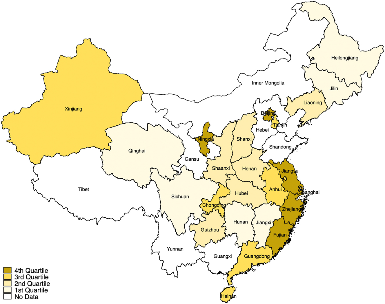
Choropleth map of litigation rates. The figure shows litigation rates in 2018 by province. Litigation rates are defined as the number of civil lawsuits in which the plaintiff used an attorney per 10,000 people. Darker shades of yellow indicate higher litigation rates.

References

Arrow, Kenneth J. 1965. Aspects of the Theory of Risk-Bearing. Helsinki: Yrjö Jahnssonin Säätiö.Search in Google Scholar

Baker, Tom. 2005. “Liability Insurance as Tort Regulation: Six Ways that Liability Insurance Shapes Tort Law in Action.” Connecticut Insurance Law Journal 12: 1–48.Search in Google Scholar

Baker, Tom, and Peter Siegelman. 2013. “The Law and Economics of Liability Insurance: A Theoretical and Empirical Review.” In Research Handbook on the Economics of Torts, edited by J. H. Arlen, 169–96. Cheltenham: Edward Elgar Publishing.10.4337/9781781006177.00015Search in Google Scholar

Beck, Thorsten, and Ian Webb. 2003. “Economic, Demographic, and Institutional Determinants of Life Insurance Consumption Across Countries.” The World Bank Economic Review 17 (1): 51–88. https://doi.org/10.1093/wber/lhg011.Search in Google Scholar

Belotti, Federico, Gordon Hughes, and Andrea P. Mortari. 2017. “Spatial Panel-Data Models Using Stata.” The Stata Journal 17 (1): 139–80. https://doi.org/10.1177/1536867x1701700109.Search in Google Scholar

Born, Patricia, and Douglas Bujakowski. 2021. “Economic Transition and Insurance Market Development: Evidence from Post-Communist European Countries.” The Geneva Risk and Insurance Review 46 (1): 1–37. https://doi.org/10.1057/s10713-021-00066-3.Search in Google Scholar

Bovbjerg, Randall R. 1994. “Liability and Liability Insurance: Chicken and Egg, Destructive Spiral, or Risk and Reaction.” Texas Law Review 72 (8): 1655–705.Search in Google Scholar

Brokešová, Zuzana, and Ingrid Vachálková. 2016. “Macroeconomic Environment and Insurance Industry Development: The Case of Visegrad Group Countries.” Ekonomická revue – Central European Review of Economic Issues 19: 63–72.Search in Google Scholar

Bujakowski, Douglas, and Shinichi Kamiya. 2023. “Estimating Spillover Effects in Property and Casualty Insurance Consumption.” North American Actuarial Journal 27 (2): 355–79. https://doi.org/10.1080/10920277.2022.2086141.Search in Google Scholar

Chin, Audrey, and Mark A. Peterson. 1985. Deep Pockets, Empty Pockets: Who Wins in Cook County Jury Trials. Santa Monica: RAND Corporation. https://www.rand.org/content/dam/rand/pubs/reports/2007/R3249.pdf (accessed December 28, 2024).Search in Google Scholar

D’Arcy, Stephen P. 1994. “The Dark Side of Insurance.” In Insurance, Risk Management, and Public Policy: Essays in Memory of Robert I. Mehr, edited by S. G. Gustavson, and S. E. Harrington, 163–81. Dordrecht: Springer.Search in Google Scholar

Danzon, Patricia M. 1980. The Disposition of Medical Malpractice Claims. Santa Monica: RAND Corporation. https://www.rand.org/content/dam/rand/pubs/reports/2006/R2622.pdf (accessed December 28, 2024).Search in Google Scholar

Elhorst, J. Paul. 2010. “Applied Spatial Econometrics: Raising the bar.” Spatial Economic Analysis 5 (1): 9–28. https://doi.org/10.1080/17421770903541772.Search in Google Scholar

Esho, Neil, Anatoly Kirievsky, Damien Ward, and Ralf Zurbruegg. 2004. “Law and the Determinants of Property-Casualty Insurance.” Journal of Risk and Insurance 71 (2): 265–83. https://doi.org/10.1111/j.0022-4367.2004.00089.x.Search in Google Scholar

Feyen, Erik, Rodney Lester, and Roberto de Rezende Rocha. 2011. “What Drives the Development of the Insurance Sector? An Empirical Analysis Based on a Panel of Developed and Developing Countries.” Journal of Financial Perspectives 1 (1): 117–39.10.1596/1813-9450-5572Search in Google Scholar

Gillan, Stuart L., and Christine A. Panasian. 2015. “On Lawsuits, Corporate Governance, and Directors’ and Officers’ Liability Insurance.” Journal of Risk and Insurance 82 (4): 793–822. https://doi.org/10.1111/jori.12043.Search in Google Scholar

Halek, Martin, and Joseph G. Eisenhauer. 2001. “Demography of Risk Aversion.” Journal of Risk and Insurance 68 (1): 1–24. https://doi.org/10.2307/2678130.Search in Google Scholar

Hammitt, James K., Stephen J. Carroll, and Daniel A. Relles. 1985. “Tort Standards and Jury Decisions.” The Journal of Legal Studies 14 (3): 751–76. https://doi.org/10.1086/467797.Search in Google Scholar

Harrington, Scott E., and Patricia M. Danzon. 2000. “The Economics of Liability Insurance.” In Handbook of Insurance, edited by G. Dionne, 277–313. Boston: Kluwer Academic Publishers.10.1007/978-94-010-0642-2_9Search in Google Scholar

Kjosevski, Jordan. 2012. “The Determinants of Life Insurance Demand in Central and Southeastern Europe.” International Journal of Economics and Finance 4 (3): 237–47. https://doi.org/10.5539/ijef.v4n3p237.Search in Google Scholar

Lee, Chien-Chiang, and Yi-Bin Chiu. 2012. “The Impact of Real Income on Insurance Premiums: Evidence from Panel Data.” International Review of Economics and Finance 21 (1): 246–60. https://doi.org/10.1016/j.iref.2011.07.003.Search in Google Scholar

LeSage, James, and Robert Kelley Pace. 2009. Introduction to Spatial Econometrics. Boca Raton: Taylor and Francis.10.1201/9781420064254Search in Google Scholar

Millo, Giovanni, and Gaetano Carmeci. 2011. “Non-Life Insurance Consumption in Italy: A Sub-Regional Panel Data Analysis.” Journal of Geographical Systems 13 (3): 273–98. https://doi.org/10.1007/s10109-010-0125-5.Search in Google Scholar

Millo, Giovanni, and Gaetano Carmeci. 2015. “A Subregional Panel Data Analysis of Life Insurance Consumption in Italy.” Journal of Risk and Insurance 82 (2): 317–40. https://doi.org/10.1111/jori.12023.Search in Google Scholar

Mossin, Jan. 1968. “Optimal Multiperiod Portfolio Policies.” Journal of Business 41 (2): 215–31. https://doi.org/10.1086/295078.Search in Google Scholar

Outreville, J. François. 1990. “The Economic Significance of Insurance Markets in Developing Countries.” Journal of Risk and Insurance 57 (3): 487–504. https://doi.org/10.2307/252844.Search in Google Scholar

Outreville, J. François. 2013. “The Relationship Between Insurance and Economic Development: 85 Empirical Papers for a Review of the Literature.” Risk Management and Insurance Review 16 (1): 71–102. https://doi.org/10.1111/j.1540-6296.2012.01219.x.Search in Google Scholar

Outreville, J. François. 2015. “The Relationship Between Relative Risk Aversion and the Level of Education: A Survey and Implications for the Demand for Life Insurance.” Journal of Economic Surveys 29 (1): 97–111. https://doi.org/10.1111/joes.12050.Search in Google Scholar

Parchomovsky, Gideon, and Peter Siegelman. 2020. “The Paradox of Insurance.” All Faculty Scholarship at University of Pennsylvania Carey Law School 2158. https://scholarship.law.upenn.edu/cgi/viewcontent.cgi?article=3160&context=faculty_scholarship (accessed December 28, 2024).Search in Google Scholar

Park, Sojung, and Jean Lemaire. 2012. “The Impact of Culture on the Demand for Non-Life Insurance.” ASTIN Bulletin 42 (2): 501–27.Search in Google Scholar

Pottier, Steven W., and Robert C. Witt. 1994. “On the Demand for Liability Insurance: An Insurance Economics Perspective.” Texas Law Review 72 (8): 1681–700.Search in Google Scholar

Proost, Stef, and Jacques-Francois Thisse. 2019. “What Can Be Learned from Spatial Economics?” Journal of Economic Literature 57 (3): 575–643. https://doi.org/10.1257/jel.20181414.Search in Google Scholar

Redding, Stephen. J., and Esteban Rossi-Hansberg. 2017. “Quantitative Spatial Economics.” Annual Review of Economics 9 (1): 21–58. https://doi.org/10.1146/annurev-economics-063016-103713.Search in Google Scholar

Shavell, Steven. 1986. “The Judgment Proof Problem.” International Review of Law and Economics 6 (1): 45–58. https://doi.org/10.1016/0144-8188(86)90038-4.Search in Google Scholar

Sinn, Hans-Werner. 1982. “Kinked Utility and the Demand for Human Wealth and Liability Insurance.” European Economic Review 17 (2): 149–62. https://doi.org/10.1016/s0014-2921(82)80011-1.Search in Google Scholar

Smith, Vernon L. 1968. “Optimal Insurance Coverage.” Journal of Political Economy 76 (1): 68–93. https://doi.org/10.1086/259382.Search in Google Scholar

Syverud, Kent D. 1994. “On the Demand for Liability Insurance.” Texas Law Review 72 (8): 1629–55.Search in Google Scholar

Wooldridge, Jeffrey M. 2010. Econometric Analysis of Cross Section and Panel Data. Cambridge: The MIT Press.Search in Google Scholar

Yang, Rui. 2019. “China Liability Insurance Market Trend Report.” Swiss Re. https://www.swissre.com/dam/jcr:64625acc-dd25-4719-bf2b-935b65727ed5/China%20Liability%20Insurance%20Market%20Trend%20Report%20-%20updated.pdf (accessed December 28, 2024).Search in Google Scholar

Yu, Jihai, Robert De Jong, and Lung-Fei Lee. 2008. “Quasi-Maximum Likelihood Estimators for Spatial Dynamic Panel Data with Fixed Effects when Both N and T are Large.” Journal of Econometrics 146 (1): 118–34. https://doi.org/10.1016/j.jeconom.2008.08.002.Search in Google Scholar

Zhong, Ming, Zhenzhen Sun, Gene Lai, and Tong Yu. 2015. “Cultural Influence on Insurance Consumption: Insights from the Chinese Insurance Market.” China Journal of Accounting Studies 3 (1): 24–48. https://doi.org/10.1080/21697213.2015.1012323.Search in Google Scholar

Received: 2025-02-21

Accepted: 2025-10-09

Published Online: 2025-11-05

You are currently not able to access this content.

https://doi.org/10.1515/apjri-2025-0008

Keywords for this article

spatial model; insurance consumption; spillover effect; China