Automatic Segmentation of Insurance Rating Classes Under Ordinal Constraints via Group Fused Lasso

1 Introduction

Premium tariffs have long been used to reference general insurance premiums according to insured’s attribute information. Tariff theory has developed along with modern statistical theory. Generalized linear models (GLMs) by Nelder and Wedderburn (1972) can model expected claim frequency and severity for each risk profile and estimate them from past claims data. Many rating factors can be incorporated into GLMs, and the optimal model can be chosen via model selection methods such as cross validation. However, some rating factors, such as the insured’s age, address and occupation, often have too many categories to obtain reliable estimates for their individual categories. In addition, complex tariffs with many categories may increase the operational risk of applying incorrect premiums. Hence, rating categories are often grouped into fewer categories which have similar risk levels in practice.

However, finding the optimal grouping of the rating categories based on a model selection criterion is difficult, because of the immense computational workload required to process almost infinite number of grouping combinations. In such cases, rating categories have been grouped based on simplicity, sales strategies, and actuarial decision-making. Some studies have applied clustering methods to reduce the rating factors and categories (e.g. Pelessoni and Picech 1998; Guo 2003; Sanche and Lonergan 2006; Yao et al. 2016). Nonetheless, most of them separate the inference and clustering procedures, which would not provide solutions satisfying both the inference criterion and the clustering criterion simultaneously.

In recent years, sparse regularization techniques, originating from the least absolute shrinkage and selection operator (lasso) by Tibshirani (1996), have been developed to enable fast variable selection when processing big data. Particularly, the fused lasso by Tibshirani et al. (2005) and its extensions are useful for automatically integrating the categories of factors by optimizing an objective function with L1 regularization terms for the differences between the regression coefficients on adjacent categories. Fujita et al. (2020) implemented the one-dimensional fused lasso for GLMs by introducing dummy variables with the ordinary lasso which indicate whether the category in each data comes before or after some change-points. Devriendt et al. (2021) proposed an efficient algorithm for sparse regression with multi-type regularization terms including the lasso and fused lasso with an application to insurance pricing analytics. Bleakley and Vert (2011) proposed the group fused lasso on a line to detect multiple change-points in multi-task learning and Alaíz, Barbero, and Dorronsoro (2013) generalized that approach to the group fused lasso on general adjacent graphs with an efficient algorithm. Nomura (2017) used the group fused lasso to integrate rating categories consistently between expected claim frequency and expected claim severity, which are modeled separately using GLMs.

In this paper, we enhance the group fused lasso used in Nomura (2017) by imposing ordinal constraints on the regression coefficients in the GLMs to meet practical requirements such as the bonus–malus system in automobile insurance. The optimization problem for parameter inference can be solved by the alternating direction multiplier method (ADMM), which is modified from the one in Nomura (2017) to satisfy the ordinal constraints. Interaction of variables with the ordinal constraints can also be incorporated into our model and solved by the modified ADMM.

The remainder of this article is organized as follows; The GLMs for claim frequency and claim severity are introduced in Section 2. The group fused lasso and the ADMM as its optimization algorithm proposed in Nomura (2017) are presented in Sections 3 and 4, respectively. The ordinal constraints on the group fused lasso and the modified ADMM are proposed in Section 5. An application of the proposed methods to motorcycle insurance data is presented in Section 6. The conclusion is finally presented in Section 7.

2 Generalized Linear Models for Claim Frequency and Severity

This section introduces the generalized linear models for insurance pricing as the fundamental models used in this study. Consider p rating factors whose numbers of categories are n ₁, …, n _p , respectively. There are T policies or a group of policies with the same factor categories. Let x _t1, …, x _tp denote the categories to which the tth policy or group of policies belongs. A generalized linear model (GLM) is an extended version of an ordinary linear regression model that can handle probability distributions in the exponential dispersion model and nonlinear link functions. In the exponential dispersion model, the probability mass functions or probability density functions of the observations a ₁, …, a _T have a common form expressed as

where θ _t denotes the parameter related to the mean of the observation a _t of the tth policy and ϕ is the dispersion parameter related to the variance of all the observation a ₁, …, a _T across the policies. Moreover, d _t is the weight assigned to the tth policy and affects the variance of the observation a _t . The function b(θ _t ) is assumed to be twice-differentiable and the function c(a _t , d _t , ϕ) is a normalization constant that makes the sum of probabilities equal to one irrespective of the value of θ _t . The mean and variance of a _t are expressed using the first-order derivative b′ and second-order derivative b″ of the function b as follows:

Ratemaking in general insurance often involves estimating the expected claim frequency and expected claim severity, separately, rather than estimating the expected total claim cost as the pure premium directly. Therefore, we next introduce the exponential dispersion models for claim frequency and claim severity, respectively.

The Poisson distribution with the following probability mass function is often applied to the number of claims per policy:

where z _t and w _t are the number of claims and the exposure of the tth policy, respectively. Then, it holds that E ( z t ) = V a r ( z t ) = w t μ t ( 1 ) and hence μ t ( 1 ) represents the expected claim frequency per exposure. Although the Poisson distribution itself does not belong to the exponential dispersion model, the probability distribution of the claim frequency z _t /w _t per exposure becomes the relative Poisson distribution which belongs to the exponential dispersion model (1) with θ t ( μ t ( 1 ) ) = log ⁡ μ t ( 1 ) and ϕ = 1.

Given the number of claims z _t from the tth policy, the gamma distribution with the following probability density function can be fitted to the claim severity:

where y _t is the mean severity of the claims from the tth policy. Then, we have E ( y t ) = μ t ( 2 ) and V a r ( y t ) = ϕ μ t ( 2 ) 2 / z t . The gamma distribution belongs to the exponential dispersion model (1) with w _t = z _t and θ t ( μ t ( 2 ) ) = − 1 / μ t ( 2 ) . Thus, the product of the expected claim frequency μ t ( 1 ) and the expected claim severity μ t ( 2 ) in (3), (4) provides the expected total claim cost, i.e. the pure premium, of the tth policy.

Let x _ti t = 1, …, T, i = 1, …, p denote the category of the ith factor to which the tth policy belongs. In a generalized linear model, the mean parameter μ _t found in (3) and (4) is formulated by:

where β ₀ is the intercept and β _ij is the regression coefficient for the jth category of the ith factor. Note that each factor has one reference category whose regression coefficient is fixed at zero. The function g is a differentiable monotonic function called a link function. When the link function is an identity function g(y) ≡ y, the mean parameter μ _t is just the right side of Equation (5). In contrast, when the link function is a logarithmic function g(y) = logy, the mean parameter μ _t is formulated by

In this case, exp(β _ij ) represents the relative risk of the jth category from the reference category in the ith factor.

The parameters in GLMs are typically estimated via the maximum likelihood method. Let β = ( β 0 , β 11 , … , β 1 n 1 , … , β p 1 , … , β p n p ) denote the set of regression coefficients including the intercept. Then, the log-likelihood of the parameter set ( β , ϕ) for the exponential dispersion model (1) is defined by

where θ t ( β ) = b ′ − 1 ( μ t ) = b ′ − 1 ◦ g − 1 ( β 0 + β 1 x t 1 + ⋯ + β p x tp ) . The maximum likelihood estimate ( β ̂ , ϕ ̂ ) of the parameter set ( β , ϕ) is given by

Particularly, the maximum likelihood estimate β ̂ of the regression coefficients β can be obtained by the following simple formula, irrespective of the value of ϕ:

Therefore, we can first estimate the regression coefficients β by (9) and then estimate the dispersion parameter ϕ by optimizing the log-likelihood (7). Regarding the Poisson distribution (3), the dispersion parameter ϕ is fixed at one, as mentioned above, and the regression coefficients β are estimated by

Regarding the gamma distribution (4), the estimates (9) of the regression coefficients become

These optimization problems can be solved quickly through optimization methods, which are typically gradient-based methods such as Newton’s method. If we apply the logarithmic link function g(y) = log(y), the objective functions in (10) and (11) become strictly convex functions, each of which has a unique local minimum that can be obtained by ordinary optimization methods.

3 Automatic Segmentation of Rating Categories via the Group Fused Lasso

We have introduced the GLMs to estimate expected claim frequency and expected claim severity from claim data. However, when using rating factors with so many categories or interactions of the factors, we have so many regression coefficients that their estimates might have large errors. In such cases, categories with similar risk levels are often integrated into groups in practice. Thus, in this section, we introduce the group fused lasso proposed by Bleakley and Vert (2011) to facilitate automatic segmentation of categories in rating factors.

For sake of simplicity, let the first factor consist of a large number of categories V = {1, …, n ₁} which need to be integrated into fewer groups for ratemaking. We define a set of pairs of adjacent categories E = {e ₁, …, e _m } ⊆ V × V as candidates of pairs to be integrated. The set (V, E) is often referred as an undirected graph where V is a set of vertices and E is a set of edges. The fused lasso on the graph (V, E) is a regularization technique to estimate the regression coefficients by solving the following optimization problem:

where the first term q( β , ϕ; y _t , w _t ) is a loss function, which becomes the negative log-likelihood function in GLMs. The second term is the L1 regularization term on the differences between the pairs of coefficients (β _1u , β _1v ) of adjacent categories (u, v) ∈ E, which encourages the coefficients β _1u , β _1v to have similar or even the same values. The categories whose regression coefficients are estimated at the same value are regarded as a group in rating-class segmentation. The weight κ on the second term is called a regularization parameter, and adjusts the impact of the regularization term.

Using the fused lasso (12), expected claim frequency and expected claim severity are estimated separately and hence would have different groupings. Since the pure premium is obtained by the product of expected claim frequency and expected claim severity, it is more desirable to determine grouping of rating classes consistently between expected claim frequency and expected claim severity. Therefore, we introduce the group fused lasso to estimate expected claim frequency and expected claim severity simultaneously by solving the following optimization problem:

where f ₁ and f ₂ are the probability mass function (3) of the Poisson distribution and the probability density function (4) of the gamma distribution, respectively. The loss function in Equation (13) is a negative log-likelihood for the joint distribution of the number of claims z _t and claim severity y _t . The regression coefficients β ⁽¹⁾ and β ⁽²⁾ are involved with the expected claim frequency μ t ( 1 ) ( β ( 1 ) ) = g − 1 ( β 0 ( 1 ) + β 1 x t 1 ( 1 ) + ⋯ + β p x tp ( 1 ) ) and the expected claim severity β ( 2 ) = g − 1 ( β 0 ( 2 ) + β 1 x t 1 ( 2 ) + ⋯ + β p x tp ( 2 ) ) , respectively, and combined into β = ( β ⁽¹⁾, β ⁽²⁾). We also concatenate the same components of β ⁽¹⁾ and β ⁽²⁾ for the category u of the first factor into β 1 u = ( β 1 u ( 1 ) , β 1 u ( 2 ) ) and introduce a regularization term ‖ β 1 u − β 1 v ‖ 2 = ( β 1 u ( 1 ) − β 1 v ( 1 ) ) 2 + ( β 1 u ( 2 ) − β 1 v ( 2 ) ) 2 for them to encourage the differences of coefficient pairs β 1 u = ( β 1 u ( 1 ) , β 1 u ( 2 ) ) and β 1 v = ( β 1 v ( 1 ) , β 1 v ( 2 ) ) to be zero simultaneously. Thus, we can determine the segmentation of rating categories simultaneously for the expected claim frequency and expected claim severity. The value of the regularization parameter κ is typically selected from discretized candidate values by cross validation methods. In N-fold cross validation, all the data (policies) are partitioned into N groups T 1 , … , T N ⊂ { 1 , … , T } . For k = 1, …, N, we obtain the estimates β ̂ − k , ϕ ̂ − k by (13) from all the data except for those in the kth group T k and fit them to the kth group T k to evaluate the validation error. As for the validation error, although we can use the sum of negative log-likelihoods for the observed claim frequency z _t and claim severity y _t , we adopt the negative log-likelihood of the observed total claim cost s _t = y _t z _t given by

where

This probability distribution of the total claim cost s _t = y _t z _t is a compound Poisson distribution with the gamma distribution (4) and known as the Tweedie distribution proposed by Tweedie (1984). By using the Tweedie distribution, we intend to evaluate predictive performance for the total claim costs directly. Finally, the value which minimizes the validation error is selected for the regularization parameter κ.

4 Optimization Algorithm for Group Fused Lasso

This section describes the algorithm to solve the optimization problem (13) introduced in the previous section. The optimization problem (8) without regularization terms can be quickly solved by using gradient-based methods such as Newton’s method and its variants. However, gradient-based methods are not applicable to the objective function in (13) whose gradients do not exist if one of the regularization terms takes exact zero. Some optimization algorithms have been proposed for the group fused lasso; the block coordinate descent method by Bleakley and Vert (2011), the alternating direction method of multipliers (ADMM) by Wahlberg et al. (2012), and the active set projected Newton method by Wytock, Sra, and Kolter (2014). The block coordinate descent method is only applicable to group fused lasso on a chain graph which can be reduced into an ordinary grouped lasso. The active set projected Newton method proposed can achieve solutions quickly for the group fused lasso on a general graph, but is difficult to apply to general loss functions other than the residual sum of squares. In contrast, the ADMM is highly versatile and can be applied to general convex loss functions and group fused lasso on general graphs. Thus, we introduce the ADMM to solve (13).

The ADMM is an optimization method that extends the Lagrange multiplier method, in which augmented Lagrangian terms are added to the objective function. Before introducing the augmented Lagrangian, we rewrite the optimization problem (13) into the following equivalent constrained optimization problem:

where ξ l = ( ξ l ( 1 ) , ξ l ( 2 ) ) is a two-dimensional dummy variable, which have to coincide with the difference between β 1 e l 1 = ( β 1 e l 1 ( 1 ) , β 1 e l 1 ( 2 ) ) and β 1 e l 2 = ( β 1 e l 2 ( 1 ) , β 1 e l 2 ( 2 ) ) , and e _l = (e _l1, e _l2) ∈ E ⊆ V × V is the lth edge in the undirected graph (V, E) on the categories of the first factor V = {1, …, n ₁}. We now introduce the augmented Lagrangian for solving the constrained optimization problem (16). The ordinary Lagrange multipliers method adds inner products − ⟨ β 1 e l 1 − β 1 e l 2 − ξ l , λ l ⟩ of the constraints β 1 e l 1 − β 1 e l 2 − ξ l restricted to be zero and the Lagrange multipliers λ l = ( λ l ( 1 ) , λ l ( 2 ) ) for l = 1, …, m, instead of removing the constraints in (16). In the augmented Lagrangian method, the L2 norms ρ 2 ‖ β 1 e l 1 − β 1 e l 2 − ξ l ‖ 2 2 with a common weight ρ/2 are further added to the objective function. Here we use ρ/2 instead of ρ because ρ/2 is used in most of the literatures using ADMM, including Wahlberg et al. (2012) and Wytock, Sra, and Kolter (2014). By optimizing the new objective function without constraints, we can obtain the same optimal solution as that of the constrained optimization problem (16). In the ADMM, the original parameter set ( β , ϕ), the dummy variables ξ = ( ξ ₁, …, ξ _m ), and the Lagrange multipliers λ = ( λ ₁, …, λ _m ) are alternately optimized as follows:

The regularization terms κ ∑ l = 1 m ‖ ξ l ‖ 2 including none of ( β , ϕ) are ignored in (17), while the loss functions including none of ξ are ignored in (18). The objective function in (17) is differentiable and hence gradient-based methods can be used to obtain the optimal solution of (17) quickly. The solution of the optimization problem in (18) can be analytically obtained by

where η l = ρ ( β 1 e l 1 new − β 1 e l 2 new ) − λ l . In (19), the constant ρ adjusts the step size of updating λ = ( λ ₁, …, λ _m ). By updating the values of the parameters into ( β ^new, ϕ ^new, ξ ^new, λ ^new) repeatedly, they will converge to the optimal solution.

5 Group Fused Lasso under Ordinal Constraints

We have introduced the GLMs with the group fused lasso proposed in Nomura (2017) to estimate expected claim costs for automatically grouped rating classes. In practice, some ordinal constraints are often imposed to insurance premiums such as monotonic constraints on bonus–malus classes in automobile insurance. To obtain estimates that satisfy such constraints, we propose the group fused lasso for the GLMs under monotonic constraints and a modification of the ADMM given in the previous section.

We inherit the notation in the previous sections and consider the following optimization problem for grouping expected claim frequency and expected claim severity simultaneously under ordinal constraints.

The sign of inequality in constraints ≥ represents the inequality applied to each element, i.e., x ≥ y for x = (x ₁, …, x _n ) and y = (y ₁, …, y _n ) means x _i ≥ y _i  (i = 1, …, n). The optimization problem (21) can be solved by the ADMM constructed in a similar manner with that in the previous section. First, we rewrite the optimization problem (21) into the following equivalent optimization problem:

Then, the update equations of the ADMM to solve (22) can be obtained by adding the constraints ξ _l ≥ 0 to those in the previous section:

The objective function in (23) is the same as that in (17) and hence gradient-based methods can be used. The solution of the optimization problem in (24) can be analytically obtained by

where η l + = ( max η l ( 1 ) , 0 , max η l ( 2 ) , 0 ) denotes the element-wise positive part of η l = ( η l ( 1 ) , η l ( 2 ) ) = ρ ( β 1 e l 1 new − β 1 e l 2 new ) − λ l . In (25), the constant ρ adjusts the step size in updating λ = ( λ ₁, …, λ _m ). By updating the values of parameters into ( β ^new, ϕ ^new, ξ ^new, λ ^new) repeatedly, they will converge to the optimal solution.

6 Application to Motorcycle Insurance Data

In this section, we apply the proposed method to claim data of the Swedish motorcycle insurance in Ohlsson and Johansson (2010). The data contain attribute information, exposure, number of claims, and total claim cost of each policy. We used the following variables in the dataset:

1. The owner’s age, between 0 and 99.

2. The EV-rate class classified by so called the EV ratio (=engine output (kW) ÷ (vehicle weight (kg) + 75) × 100).^[1]

3. The city-size class classified by the scale and location of cities and towns.^[2]

4. The Bonus–malus class taking values from 1 to 7. The class starts from 1 for a new driver, increases by 1 for each claim-free year, and decreases by 2 for each claim.

5. The Exposure or the number of policy years.

6. The number of claims.

7. The claim cost in Swedish Kronor.

Table 1 shows the summary statistics aggregated by factor. Here, the claim frequency is calculated by dividing the number of claims by the exposure, and the claim severity is calculated by dividing the claim cost by the number of claims. As shown in Table 1, the claim frequency tends to be higher for younger owners, higher EV-rates (engine output), and larger cities. In contrast, the claim severity is relatively high for 20–59 year-old owners, the middle EV-rate (class 3), and large cities. Note that the claim frequency and severity do not always decline as the bonus–malus class increases.

Throughout this section, we fit the Poisson GLM (3) and the gamma GLM (4) to the number of claims y _t and the claim severity z _t (=the claim cost ÷ the number of claims), respectively, with log link g(μ) = logμ and p = 4 risk factors: the owner’s age x _t1, EV-rate class x _t2, city-size class x _t3, and bonus–malus class x _t4 of the tth policy. The owner’s age x _t1 has n ₁ = 100 (0–99 years old) grades, whereas the other factors x _t2, x _t3, x _t4 have n ₂ = n ₃ = n ₄ = 7 grades for each. In particular, we apply the group fused lasso on several types of underlying graphs with monotonic constraints for the EV-rate and Bonus–malus classes in the following subsections.

6.1 Group Fused Lasso for Single Factors with Monotonic Constraints

First, we incorporated the group fused lasso for each factor into the GLMs and considered the following optimization problem to estimate the parameters:

(27) min ( β , ϕ ) − ∑ t = 1 T log f 1 ( z t ; μ t ( 1 ) ( β ( 1 ) ) , w t ) + log f 2 ( y t ; μ t ( 2 ) ( β ( 2 ) ) , z t , ϕ )   + κ ∑ i = 1 4 ∑ k = 1 n i − 1 ‖ β i , k + 1 − β i , k ‖ 2 , s.t.   β 2 , k + 1 − β 2 , k ⪰ 0 , k = 1 , … , n 2 − 1 ,     β 4 , k + 1 − β 4 , k ⪯ 0 , k = 1 , … , n 4 − 1 ,

where β i , k = β i , k ( 1 ) , β i , k ( 2 ) is the regression coefficients on the kth grade of the ith factor for expected claim frequency and expected claim severity, respectively. An adjacency graph (V _i , E _i ) with vertex set V _i = {1, …, n _i } and edge set E _i = {(k + 1, k)|k = 1, …, n _i − 1} was applied in the group fused lasso for each factor i = 1, 2, 3, 4. Because the EV-rate classes are in an ascending order of EV rate, a higher claim cost is expected in the policy with the higher EV-rate class. Therefore, we imposed a monotonic constraint β 2,1 ⪯ β 2,2 ⪯ … ⪯ β 2 , n 2 on the EV-rate classes. We also introduced a monotonic constraint β 4,1 ⪰ β 4,2 ⪰ … ⪰ β 4 , n 4 on the bonus–malus classes since the bonus–malus class rises by no-claim periods and falls by claims. We illustrate the underlying graphs of the group fused lasso in Figure 1. Each pair of adjacent classes without constraints is connected by an undirected edge, whereas each pair of adjacent classes with an ordinal constrain is connected by a directed edge from the class with the smaller coefficient to the class with the larger coefficient.

Figure 1:

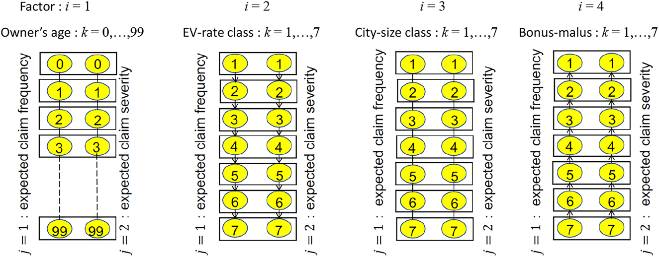
Underlying adjacent graphs of the group fused lasso for single factors.

To solve the optimization problem (27), we first rewrite it into the following equivalent optimization problem:

(28) min ( β , ϕ , ξ ) − ∑ t = 1 T log f 1 ( z t ; μ t ( 1 ) ( β ( 1 ) ) , w t ) + log f 2 ( y t ; μ t ( 2 ) ( β ( 2 ) ) , z t , ϕ ) + κ ∑ i = 1 4 ∑ k = 1 n i − 1 ‖ ξ i , k ‖ 2 , s.t.   ξ i , k = β i , k + 1 − β i , k , i = 1,3 , k = 1 , … , n i − 1 , ξ 2 , k = β 2 , k + 1 − β 2 , k ⪰ 0 , k = 1 , … , n 2 − 1 , ξ 4 , k = β 4 , k + 1 − β 4 , k ⪯ 0 , k = 1 , … , n 4 − 1 .

Then, the update equations to solve (28) are constructed in the same manner as in the previous sections and given by

(29) ( β new , ϕ new ) = arg⁡min ( β , ϕ ) − ∑ t = 1 T log f 1 ( z t ; μ t ( 1 ) ( β ( 1 ) ) , w t ) + log f 2 ( y t ; μ t ( 2 ) ( β ( 2 ) ) , z t , ϕ ) + ∑ i = 1 4 ∑ k = 1 n i − 1 − 〈 β i , k + 1 − β i , k − ξ i , k , λ i , k 〉 + ρ i 2 ‖ β i , k + 1 − β i , k − ξ i , k ‖ 2 2 ,

(30) ξ i , k new = arg⁡min ξ i , k κ ‖ ξ i , k ‖ 2 − 〈 β i , k + 1 new − β i , k new − ξ i , k , λ i , k 〉 + ρ i 2 ‖ β i , k + 1 new − β i , k new − ξ i , k ‖ 2 2 , i = 1,3 , k = 1 , … , n i − 1 ,

(31) ξ 2 , k new = arg⁡min ξ 2 , k ⪰ 0 κ ‖ ξ 2 , k ‖ 2 − 〈 β 2 , k + 1 new − β 2 , k new − ξ 2 , k , λ 2 , k 〉 + ρ 2 2 ‖ β 2 , k + 1 new − β 2 , k new − ξ 2 , k ‖ 2 2 , k = 1 , … , n 2 − 1 ,

(32) ξ 4 , k new = arg⁡min ξ 4 , k ⪯ 0 κ ‖ ξ 4 , k ‖ 2 − 〈 β 4 , k + 1 new − β 4 , k new − ξ 4 , k , λ 4 , k 〉 + ρ 4 2 ‖ β 4 , k + 1 new − β 4 , k new − ξ 4 , k ‖ 2 2 , k = 1 , … , n 4 − 1 ,

(33) λ i , k new = λ i , k − ρ i β i , k + 1 new − β i , k new − ξ i , k new , i = 1,2,3,4 , k = 1 , … , n i − 1 ,

where ρ _i is basically set at κ for i = 1, 2, 3, 4 but partially adjusted as ρ ₃ = max{10κ, 10} when κ < 10 to accelerate convergence to the optimal solution. The optimization in Equations (30)–(32) are analytically solved as described in the previous sections. First, the analytical solution of (30) is given by

(34) ξ i , k new = 1 − κ ‖ η i , k ‖ 2 η i , k ρ i   if  ‖ η i , k ‖ 2 > κ , 0 , if  ‖ η i , k ‖ 2 ≤ κ ,   i = 1,3 , k = 1 , … , n i − 1 ,

where η i , k = ρ i ( β i , k + 1 new − β i , k new ) − λ i , k for i = 1, 3 and k = 1, …, n _i . Second, the analytical solution of (31) is given by

(35) ξ 2 , k new = 1 − κ ‖ η 2 , k + ‖ 2 η 2 , k + ρ 2   if  ‖ η 2 , k + ‖ 2 > κ , 0 , if  ‖ η 2 , k + ‖ 2 ≤ κ ,   k = 1 , … , n 2 − 1 ,

where η 2 , k + = ( max η 2 , k ( 1 ) , 0 , max η 2 , k ( 2 ) , 0 ) denotes the element-wise positive part of η 2 , k = ( η 2 , k ( 1 ) , η 2 , k ( 2 ) ) = ρ 2 ( β 2 , k + 1 new − β 2 , k new ) − λ 2 , k for k = 1, …, n ₂. Third, the analytical solution of (32) is given by

(36) ξ 4 , k new = 1 − κ ‖ η 4 , k − ‖ 2 η 4 , k − ρ 4   if  ‖ η 4 , k − ‖ 2 > κ , 0 , if  ‖ η 4 , k − ‖ 2 ≤ κ ,   k = 1 , … , n 4 − 1 ,

where η 4 , k − = ( min η 4 , k ( 1 ) , 0 , min η 4 , k ( 2 ) , 0 ) denotes the element-wise negative part of η 4 , k = ( η 4 , k ( 1 ) , η 4 , k ( 2 ) ) = ρ 4 ( β 4 , k + 1 new − β 4 , k new ) − λ 4 , k for k = 1, …, n ₄.

We selected the value of the regularization parameter κ by five-fold cross validation with the validation error (14), which is the negative log-likelihood of the total claim costs in the validation data, from 100 grid points κ j = κ ̄ 1 0 − 3 j 99 for j = 99, 98, …, 0 where κ ̄ is the lowest limit of κ at which all the regression coefficients are estimated to be zero.

The validation error for each candidate value of κ is shown in Figure 2 and takes a minimum value of 9462.0 when κ = 14.9 as indicated by the vertical dotted line. Therefore, we adopted κ = 14.9 and estimated the parameters from all the data. From the estimates β ̂ 0 = β ̂ 0 ( 1 ) , β ̂ 0 ( 2 ) of the intercepts, we obtain the expected claim frequency exp ( β ̂ 0 ( 1 ) ) = 0.0087 (claim/year), expected claim severity exp ( β ̂ 0 ( 2 ) ) = 21021 (Krone/claim), and expected total claim cost (pure premium) exp ( β ̂ 0 ( 1 ) + β ̂ 0 ( 2 ) ) = 183 (Krone/year) for the policies belonging to the reference classes (owner’s age = 30, EV-rate class = 3, city-size class = 4, and bonus–malus class = 5). Moreover, from the estimates β ̂ i , k = β ̂ i , k ( 1 ) , β ̂ i , k ( 2 ) of the regression coefficients, we calculated the relative expected claim frequency exp ( β ̂ i , k ( 1 ) ) , relative expected claim severity exp ( β ̂ i , k ( 2 ) ) , and relative expected total claim cost exp ( β ̂ i , k ( 1 ) + β ̂ i , k ( 2 ) ) of the kth category from the reference category in the ith factor as shown in Tables 2 –4 and Figure 3. Note that the regression coefficients on the bonus–malus classes are all estimated to be zero and omitted in the tables.

Figure 2:

Cross validation errors for candidate values of regularization parameter κ.

Table 2:

Estimates of relative expected claim frequency, relative expected claim severity, and relative expected total claim cost for 14 groups of owner’s age.

Owner’s age	Relative expected	Relative expected	Relative expected
	claim frequency	claim severity	total claim cost
0–24	2.090	0.779	1.627
25	1.636	1.044	1.708
26	1.609	1.067	1.716
27	1.437	1.048	1.506
28	1.260	1.072	1.350
29	1.092	1.031	1.126
30	1.000	1.000	1.000
31–33	0.705	0.942	0.664
34	0.624	0.942	0.588
35	0.504	0.954	0.481
36–39	0.465	0.942	0.439
40–42	0.403	0.911	0.367
43,44	0.396	0.899	0.356
45–99	0.361	0.789	0.285

Table 3:

Estimates of relative expected claim frequency, relative expected claim severity, and relative expected total claim cost for three groups of EV-rate classes.

EV-rate class	Relative expected	Relative expected	Relative expected
	claim frequency	claim severity	total claim cost
1–4	1.000	1.000	1.000
5	1.313	1.000	1.313
6,7	2.023	1.000	2.023

Table 4:

Estimates of relative expected claim frequency, relative expected claim severity, and relative expected total claim cost for four groups of city-size classes.

City-size class	Relative expected	Relative expected	Relative expected
	claim frequency	claim severity	total claim cost
1	4.151	1.552	6.443
2	2.539	1.493	3.791
3	1.522	1.147	1.747
4–7	1.000	1.000	1.000

Figure 3:

Estimates of relative expected claim frequency, relative expected claim severity, and relative expected total claim cost for owner’s age.

In Table 2 and Figure 3, the 100 categories of owner’s age were integrated into 14 groups; two of them contain wide ranges of younger ages 0–24 and older ages 45–99, respectively, and eight of them around 30 consist of single ages, which indicates that there are significant differences in insurance risk between those ages.

The estimated expected claim frequency decreases monotonically with respect to the owner’s age and its difference is up to 5.8 times. In contrast, the estimated expected claim severity is the lowest in the youngest class 0–24 and the highest in late 20s, whose difference is only 1.4 times. Consequently, the product of them – the estimated expected total cost of claims – has its peak at 26, monotonically decreases after 26, and has six-fold difference at most.

The EV-rate classes over and under the class 5 were integrated, respectively, which results in three groups of the EV-rate classes. There is two-fold difference in the estimated expected claim frequency but no difference in the estimated expected claim severity between the first and the last groups.

Regarding the city-size classes, the classes 4–7 were integrated into one group and the others remained as single classes. Both the estimated expected claim frequency and estimated expected claim severity decrease monotonically with respect to the city-size classes and their difference is up to 4.2 and 1.6 times, respectively, which results in the difference up to 6.4 times in the estimated expected total cost of claims.

References

Alaíz, C. M., Á. Barbero, and J. R. Dorronsoro. 2013. “Group Fused Lasso.” In Artificial Neural Networks and Machine Learning – ICANN 2013. ICANN 2013. Lecture Notes in Computer Science, vol. 8131, edited by V. Mladenov, P. Koprinkova-Hristova, G. Palm, A. E. P. Villa, B. Appollini, and N. Kasabov, 66–73. Berlin: Springer.10.1007/978-3-642-40728-4_9Search in Google Scholar
Bleakley, K., and J. P. Vert. 2011. “The Group Fused Lasso for Multiple Change-point Detection.” In Working Paper. Also available at http://arxiv.org/abs/1106.4199v1.Search in Google Scholar
Devriendt, S., K. Antonio, T. Reynkens, and R. Verbelen. 2021. “Sparse Regression with Multi-type Regularized Feature Modeling.” Insurance: Mathematics and Economics 96: 248–61. https://doi.org/10.1016/j.insmatheco.2020.11.010.Search in Google Scholar
Fujita, S., T. Tanaka, K. Kondo, and H. Iwasawa. 2020. “AGLM: A Hybrid Modeling Method of GLM and Data Science Techniques.” In Actuarial Colloquium Paris 2020. Also available at https://www.institutdesactuaires.com/global/gene/link.php?doc_id=16273.Search in Google Scholar
Gráinne, M., G. Taylor, and G. Miller. 2021. “Self-assembling Insurance Claim Models Using Regularized Regression and Machine Learning.” Variance 14 (1).Search in Google Scholar
Guo, L. 2003. “Applying Data Mining Techniques in Property/casualty Insurance.” In CAS 2003 Winter Forum, Data Management, Quality, and Technology Call Papers and Ratemaking Discussion Papers, 1–25. CAS.Search in Google Scholar
Nelder, J. A., and R. W. M. Wedderburn. 1972. “Generalized Linear Models.” Journal of the Royal Statistical Society: Series A 135 (3): 370–84. https://doi.org/10.2307/2344614.Search in Google Scholar
Nomura, S. 2017. “Automatic Segmentation of Rating Classes via the Group Fused Lasso (In Japanese).” JARIP (Japanese Association of Risk, Insurance and Pensions) Journal 9 (1): 10–28.Search in Google Scholar
Ohlsson, E., and B. Johansson. 2010. Non-Life Insurance Pricing with Generalized Linear Models. EAA Series, Berlin/Heidelberg: Springer.10.1007/978-3-642-10791-7Search in Google Scholar
Pelessoni, R., and L. Picech. 1998. “Some Applications of Unsupervised Neural Networks in Rate Making Procedure.” In 1998 General Insurance Convention & ASTIN Colloquium, 549–67, Glasgow.Search in Google Scholar
Sanche, R., and K. Lonergan. 2006. “Variable Reduction for Predictive Modeling with Clustering.” In Casualty Actuarial Society Forum, Winter 2006, 89–100, Salt Lake City.Search in Google Scholar
Scardapane, S., D. Comminiello, A. Hussain, and A. Uncini. 2017. “Group Sparse Regularization for Deep Neural Networks.” Neurocomputing 241: 81–9. https://doi.org/10.1016/j.neucom.2017.02.029.Search in Google Scholar
SriDaran, D., M. Sherris, A. Villegas, and J. Ziveyi. 2022. “A Group Regularization Approach for Constructing Generalized Age-Period-Cohort Mortality Projection Models.” ASTIN Bulletin 52 (1): 247–89. https://doi.org/10.1017/asb.2021.29.Search in Google Scholar
Tibshirani, R. 1996. “Regression Shrinkage and Selection via the Lasso.” Journal of the Royal Statistical Society: Series B 58 (1): 267–88. https://doi.org/10.1111/j.2517-6161.1996.tb02080.x.Search in Google Scholar
Tibshirani, R., M. Saunders, S. Rosset, J. Zhu, and K. Knight. 2005. “Sparsity and Smoothness via the Fused Lasso.” Journal of the Royal Statistical Society: Series B 67 (1): 91–108. https://doi.org/10.1111/j.1467-9868.2005.00490.x.Search in Google Scholar
Tweedie, M. 1984. “An Index Which Distinguishes between Some Important Exponential Families.” In Statistics: Applications and New Directions. Proceedings of the Indian Statistical Institute Golden Jubilee International Conference, edited by J. Ghosh, and J. Roy, 579–604. Calcutta: Indian Statistical Institute.Search in Google Scholar
Wahlberg, B., S. Boyd, M. Annergren, and Y. Wang. 2012. “An ADMM Algorithm for a Class of Total Variation Regularized Estimation Problems.” IFAC Proceedings Volumes 45 (16): 83–8. https://doi.org/10.3182/20120711-3-be-2027.00310.Search in Google Scholar
Wytock, M., S. Sra, and J. Z. Kolter. 2014. “Fast Newton Methods for the Group Fused Lasso.” In Proceedings of the Thirtieth Conference on Uncertainty in Artificial Intelligence, 888–97.Search in Google Scholar
Yao, J. 2016. “Clustering in General Insurance Pricing.” In Predictive Modeling Applications in Actuarial Science, Volume II: Case Studies in Insurance, edited by E. W. Frees, G. Meyers, and R. A. Derrig, 159–79. Cambridge: Cambridge University Press.10.1017/CBO9781139342681.007Search in Google Scholar
© 2022 the author(s), published by De Gruyter, Berlin/Boston
This work is licensed under the Creative Commons Attribution 4.0 International License.
Articles in the same Issue
- Frontmatter
- Featured Articles (Research Paper)
- Are Stay-at-Home and Face Mask Orders Effective in Slowing Down COVID-19 Transmission? – A Statistical Study of U.S. Case Counts in 2020
- The Impact of GATS on the Insurance Sector: Empirical Evidence from Pakistan
- Processing of Information from Risk Maps in India and Germany: The Influence of Cognitive Reflection, Numeracy, and Experience
- The Determinants of Credit Rating and the Effect of Regulatory Disclosure Requirements: Evidence from an Emerging Market