Hearing exotic smooth structures

1 Introduction

A very classical and well-explored subject of geometric analysis is that of hearing shapes. Following [1], it addresses the relationship between the geometry of some Riemannian manifolds and the eigenvalues of its Laplacian operator acting on functions. Some remarkable developments are presented in [2], [3], [4], [5], [6], [7], [8], [9], [10].

Shortly, this paper mainly focuses on whether two homeomorphic but not diffeomorphic smooth manifolds admit invariant metrics sharing the same basic spectrum (Definition 3). With this aim, we use the analytical machinery and example constructions appearing in [11] to compare the basic spectra of two homeomorphic but not diffeomorphic manifolds. Theorem 3 provides examples of pairs of homeomorphic but not diffeomorphic manifolds M and M′ admitting invariant metrics g M , g M ′ that can be chosen with the same basic spectrum or not. Byproducts of the theory include showing that the ring of admissible scalar curvature functions do not distinguish smooth structures for plenty of homotopy spheres, Theorem 4. This establishes the G-invariant version of the classical Kazdan–Warner problem [12] for some equivariantly related manifolds [11].

The geometric constructions in this paper are based on the following setup. We consider a special case of principal (G, H)-bibundle in which G = H. Following [13], recall that a groupoid G = (G ₁ ⇉ G ₀) is a category in which each arrow in G ₁ has an inverse. Let G and H be Lie groupoids. A manifold P with a left G-action and a right H-action which commute is called a smooth G-H-bibundle. We much benefit from the geometric constructions in [11], [14]. To know, we look to smooth manifolds P carrying commuting free G-actions whose orbit spaces M, M′ carry G-actions. We name this construction a ⋆-diagram; see Equation (2). They constitute an example of principal G-bibundle (G = H).

A ⋆-diagram M ← P → M′ promotes a Hausdorff-Morita equivalence between the G-varieties M and M′, as firstly remarked in [11] and proved in [15]. We hope our geometric realizations shed light on the study of Lie groupoid Morita equivalence via Hilsum–Skandalis maps [13], [16]. This specifies the study of leaf spaces [17], and in the particular case of Riemannian foliations, the isospectrality question for the basic Laplacian is rather natural [18]. For instance, it has been shown in [19] that the spectrum of the basic Laplacian of a Riemannian foliation can be identified with the SO(q)-invariant spectrum of its Molino quotient manifold W via the Molino frame bundle lift (which is itself a bibundle, see, e.g., [20], [21]).

Let ( X , g ) be a closed, connected d-dimensional Riemannian manifold with an effective isometric action by a compact Lie group G; ( X , g ) is also called a Riemannian G-manifold. Let W k , p ( X ) , k ∈ Z ≥ 0 , p ∈ [ 1 , ∞ ) denote the Sobolev space recovered by smooth functions on X via taking the closure of C ^∞(X) with respect to the norm:

where ∇ denotes the Levi–Civita connection of g , ∇ ^j u is the jth-covariant derivative of u, and the norm |∇ ^j u| is computed using the tensor product metric induced by g .

Once a Haar measure on G is fixed, any element u ∈ W ^k,p (X) can be averaged along G to produce a basic or invariant function u ̄ , i.e., u ̄ ( g x ) = u ̄ ( x ) for almost every x ∈ X and every g ∈ G. We denote the set of such elements by W G k , p ( X ) . Being C G ∞ ( X ) the set of smooth basic functions in (X, G), it can be shown (see e.g. [22], Lemma 5.4, p. 91]) that C G ∞ ( X ; R ) ̄ ‖ ⋅ ‖ W k , p ( M ) = W G k , p ( X ) . Throughout this manuscript, we adopt the convention W G 0 , p ( X ) = L G p ( X ) .

Let − Δ g ≔ − d i v g ( ∇ ) be the (negative of the) Riemannian Laplacian of g . It is well known that this is a formally self-adjoint, nonnegative elliptic operator, and in particular, its spectrum is a closed, countable, discrete, unbounded set consisting only of eigenvalues with finite multiplicities, which can therefore be arranged as a sequence of nonnegative real numbers 0 = λ ₀ ≤ λ ₁ ≤ λ ₂ ≤ … ↑∞. This is known as the spectrum of ( X , g ) .

In the present context, where ( X , g ) is a Riemannian G-manifold, we want to consider the subset of the spectrum consisting of eigenvalues that correspond to invariant eigenfunctions. Thus, we consider the G-invariant eigenvalue problem:

To properly guarantee the existence of a solution to Problem 1, we define:

For a deep explanation of the basics related to the Laplacian spectra on manifolds, we refer the reader to [23].

Note that the left-hand side in equation (1) is given by

where the inner product ⟨u,v⟩_1,2 is the one associated with the norm ‖ ⋅ ‖ _1,2. It can be checked, using that X is closed and connected, that the norm  ‖ u ‖ 2 ≔ ∫ X | ∇ u | 2 d μ g defines a norm on H ( X ) which is equivalent to the norm ‖ ⋅ ‖ _1,2. Associated with ‖ ⋅ ‖ we have the inner product

Hence, equation (1) is equivalent to

On the other hand, for each fixed u ∈ H G ( X ) the map

defines a linear functional with domain ( H G ( X ) , ‖ ⋅ ‖ ) . The Riesz representation theorem ensures the existence of λ > 0 and u λ * ∈ H G ( X ) such that

The principle of symmetric criticality of Palais [24] guarantees that the same holds for every v ∈ H ( X ) . Picking v = u λ * shows that u λ * = u a.e. The classical regularity theory of PDEs guarantees the existence of a smooth invariant representative u solving Problem 1, i.e., u ∈ C G ∞ ( X ) .

Definition 3 contrasts with other already present concepts in the literature. Given a Riemannian manifold X with an isometric action by a Lie group G (a Riemannian G-manifold), we know that G has a natural representation τ _G on L ²(X) where for each f ∈ L ²(X) the function τ _G (f) ≔ g·f is given by

note that, since G acts via isometries, the representation τ _G commutes with the Laplacian Δ of M. Then, two Riemannian G-manifolds X and X′ are said to be equivariantly isospectral (with respect to G) if there is a unitary map U: L ²(X) → L ²(X′) such that [25], [26]

1. U◦Δ = Δ′◦U, that is, X and X′ are isospectral,

2. U ◦ τ G = τ G ′ ◦ U , i.e., the natural representations are equivalent via U.

The notion of isospectrality presented in Definition 3 is exactly the one appearing in [27]. In [28], Sunada studies whether two finite groups H ₁, H ₂ acting on a smooth manifold X yield coinciding H _i -invariant spectrum on X. Then, in [29], Sunada’s result is generalized to connected groups. Finally, Theorem 2.5 in [27] goes beyond, stating the following:

Proposition 1 combined with Example 2 show that the conclusion in Theorem 2.5 in [27] extends to every pair of manifolds M, M′ fitting a ⋆-diagram.

Lastly, it may be the case that our appearing constructions bring insights on the following. Although two isospectral manifolds need not be isometric, further rigidity can be questioned. For instance, the result of Tanno in [8] ensures that any compact Riemannian manifold isospectral to a round sphere S n , g round is necessarily isometric to S n , g round if n ≤ 6. Up to the smooth Poincaré conjecture in dimension 4, exotic spheres appear precisely firstly when n = 7. It is still unknown whether round 7 spheres are spectrally unique (in the sense of Tanno’s result), but it is known that no exotic sphere can carry a round metric. Based on our results, we are tempted to think that the spectral-uniqueness can not occur for spheres in every dimension n ≥ 7 where an exotic sphere exists.

2 Basic spectra of G-manifolds related by ⋆-diagrams

We outline a general procedure for constructing exotic manifolds based on their classical counterparts, extensively discussed in [11], [14], [30]. This is done by considering pairs of closed manifolds M, M′ carrying effective actions by a compact Lie group G, and fitting into a so-called ⋆-diagram M ← P → M′, which essentially realize M and M′ as quotients of a single manifold P by free commuting G-actions. Many exotic manifolds fit into these diagrams, and one can then use this structure to compare their invariant geometries once invariant metrics are considered. Notably, the concept of an exotic sphere originated in the 1950s with J. Milnor’s groundbreaking work [31]. Milnor introduced a family of 7-dimensional manifolds Σ⁷ homeomorphic to the classical sphere S⁷ but not diffeomorphic.

In the diagram (2) below, which will henceforth be called a ⋆-diagram, P represents a principal G-manifold – a manifold equipped with a free action by a compact Lie group G, denoted by •. This action implies π defines a principal bundle over M with total space P. We also assume the existence of another G-action, denoted by ⋆, which is both free and commutative with •. This action makes π′ a principal bundle over M′ with total space P. We encode everything in the following:

(2)

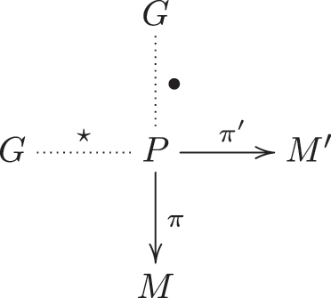
Diagram (2) yields a principal (G, G)-bundle (shortly, a principal G-bundle), [13]. We provide some explicit examples.

Example 1.

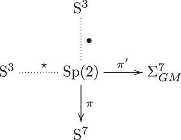
(The Gromoll–Meyer exotic sphere). This construction first appeared in [32] and was first put in a ⋆-diagram in [33] (see also [14]). Consider the compact Lie group

(3) S p ( 2 ) = a c b d ∈ S 7 × S 7 a b ̄ + c d ̄ = 0 ,

where a , b , c , d ∈ H are quaternions with their usual conjugation, multiplication, and norm. The projection π: Sp(2) → S⁷ of an element to its first row defines a principal S³-bundle with principal action:

(4) a c b d q ̄ = a c q ̄ b d q ̄ .

Gromoll–Meyer [32] introduced the ⋆-action

(5) q a c b d = q a q ̄ q c q b q ̄ q d ,

whose quotient is an exotic 7-sphere. It all fits in the following diagram

(6)

■

As the next example shows, a ⋆-diagram such as (2) does not always produce a different manifold.

Example 2.

(Pairs of diffeomorphic manifolds via ⋆-diagrams). Let M be a smooth manifold with an effective smooth action by a compact Lie group G, which we denote by ⋅. Consider the product manifold M × G with the following ⋆-action

g ⋆ ( x , g ′ ) ≔ ( g ⋅ x , g g ′ ) , x ∈ M , g , g ′ ∈ G .

Let • be the following G-action on M × G:

g • ( x , g ′ ) ≔ ( x , ( g ′ ) g − 1 ) , x ∈ M , g , g ′ ∈ G .

Both •, ⋆ are free and commuting actions on M × G. Orbit maps for such actions are, respectively, π: M × G → M, (x, g′) ↦ x, π′: M × G → M, (x, g′) ↦ (g′)⁻¹ x. We can build the corresponding ⋆-diagram

(7)

■

A new construction is given next, encompassing some cohomogeneity-one manifolds.

Example 3.

(Cohomogeneity-one manifolds). Another class of examples are the manifolds constructed in Grove–Ziller [34]. Given integers p ₊, q ₊, p ₋, q ₋ ≡ 1 (mod 4) [34], produces a cohomogeneity-one manifold ( P p − , q − , p + , q + 10 , ( S 3 ) 3 ) . We further assume that gcd(p ₋, q ₋) = gcd(p ₊, q ₊) = 1. Then one can observe that the subactions of S • 3 = S 3 × { 1 } × { 1 } and of S ⋆ 3 = { 1 } × Δ S 3 are commuting and free, where ΔS³ is the diagonal in S³ × S³. They fit in the diagram

(8)

Here, M p − , q − , p + , q + ′ is the S³-bundle over S⁴ classified by the transition function α: S³ → SO(4) defined by α(x)v = x ^k vx ^l , where k = p − 2 − p + 2 / 8 and l = − q − 2 − q + 2 / 8 . ■

As observed in [11], the actions • and ⋆ commute so that ⋆ descends to a non-trivial action on M, as well as • descends to a non-trivial action M′. Moreover, it is possible to regard M and M′ with G-invariant Riemannian metrics g M and g M ′ , respectively, such that the metric spaces M/G and M′/G are isometric.

Any smooth G × G-invariant function ϕ : P → R gives rise to smooth and G-invariant functions on both M and M′ via composing ϕ in the right with π, π′, respectively. In fact, any smooth invariant functions on M, M′ arise in this fashion. Let g P denote an arbitrary G × G-invariant metric on P, and let g M , and g M ′ be invariant Riemannian metrics on M, M′, respectively, such that the projections π, π′ define Riemannian submersions. Then, the horizontal Laplacians on M and M′ are related to the Laplacian in P as follows, see [35], Section 2.1.4, p. 53]

where H ^π stands for the mean curvature vector of the fibers according to the •-action on P and H ^π ′ to the mean curvature vector of the fibers according to ⋆. Since the ring isomorphisms C G × G ∞ ( P ) ≅ C G ∞ ( M ) ≅ C G ∞ ( M ′ ) hold, one can identify the Sobolev spaces

Consequently,

Related to Problem 2 we prove:

Our next result shows that when existing a joint invariant eigenfunction set Φ necessarily g M , g M ′ are isospectral.

An appearing question is whether we can produce invariant metrics on M and M′, which are invariant and not isospectral. We obtained the following, to be proved in Section 4.

The combination of Proposition 1 with Theorem 2 and some explicit realization of exotic manifolds equivariantly related to their classical counterpart allow us to show

With Theorem 3 in hands, it is natural to ask whether invariant geometric objects ignore the chosen smooth structure to a fixed underlined topological space. We prove

In Section 3, we both prove Theorem 4 and furnish the examples appearing in Theorem 3 and Corollary 1.

3 On the realizability of scalar curvature functions on homotopy spheres

Since Milnor introduced the first examples of exotic manifolds [31], many new exotic spaces have been produced. For instance, there are uncountable many pairwise non-diffeomorphic structures on R 4 (see [38]); exotic manifolds not bounding spin manifolds [39]; exotic projective spaces, and connected sums of exotic manifolds [11]. Following [14], [30], [33], [40], several realizations of exotic manifolds are obtained using ⋆-diagrams such as (2). This section explores the relationship between the admissibility of invariant scalar curvature functions on the manifolds M and M′, culminating in the proof of Theorem 4.

The first construction of exotic manifolds uses the classical Reeb’s Theorem to show that specific 7-dimensional total spaces of sphere bundles are homeomorphic to a standard sphere. Moreover, one can recover the smooth structure of a manifold through its space of smooth functions (see, for example, [41], Problem 1-C]). However, in the presence of a ⋆-diagram, the set of basic functions of M and M′ are naturally identified since they are naturally identified with the space of G × G-invariant functions on P, proving that the set of basic functions does not recover (M, G). Theorem 4 reinforces this fact in the sense that invariant scalar curvature functions should not distinguish smooth structures.

The remaining section presents many examples where Theorems 2–4 can be applied. We explicitly build the examples in the statements of Theorem 3 and Corollary 1.

The isomorphism ϕ in the examples Σ k 7 − (Σ⁴ⁿ⁺¹) are all of the form ϕ(h) = ghg ⁻¹ for g ∈ G only depending on p. In such cases, every pair of points x, x′, π ⁻¹(x) ∩ (π′)⁻¹(x′) ≠ ∅, have the same orbit type.

We claim that several surgeries can be done equivariantly on the manifolds resulting in these examples. Moreover, such surgeries can be done by keeping the ⋆-diagram apparatus. We give more details on the Σ k 7 -case to illustrate the assertion.

In this case, S³ acts on S⁷ as q ( a , b ) T = ( q a q ̄ , q b q ̄ ) T . This action is inherited from the representation ρ ̃ : S 3 → S O ( 8 ) defined by 2ρ ₀ ⊕ 2ρ ₁, where ρ ₀ and ρ ₁ stands for the trivial representation and the representation defined by the composition of the double-cover S³ → SO(3) and the standard action of SO(3) in R 3 . I.e., ρ ̃ is the double suspension of the bi-axial action of SO(3) in R 6 , up to a double-cover.

Note that (a,b) ^T is a fixed point of ρ ̃ whenever a , b ∈ R and consider another manifold (M ⁷, S³) with a fixed point p whose isotropy representation is ρ ₀ ⊕ 2ρ ₁. One can produce a standard degree-one equivariant map ϕ: M ⁷ → S⁷ by ‘wrapping’ S⁷ with an open ball centered at the fixed point and sending the remaining of M to the antipodal of ϕ(p). As in [11], Theorem 4.1], the induced ⋆-diagram results in M ← ϕ * P → M # Σ k 7 .

To proceed with the surgery process, note that (S⁷, S³) admits the equivariant submanifolds below. We omit the explicit embeddings and use the representation instead of G as the notation (M, G) to present more detailed information.

Except for S¹ × D ⁶ and S⁴ × D ³, every submanifold above can lie in an arbitrarily small region of a fixed Re(a). In particular, arbitrarily, many of these surgeries can be performed.

Moreover, we conclude that such surgeries can be performed by preserving infinitely many fixed points. Therefore, the above degree-one map can be considered, producing a ⋆-diagram over the new manifold M. Although the connected sum applied to this context seems ad-hoc, the resulting manifold (ϕ*P)/G = M#Σ is the same manifold one obtains by performing the same surgeries on Σ. ■

4 The proof of Theorem 2

In this last section, we prove Theorem 2. Let M ← P → M′ denote a ⋆-diagram with structure group G compact and connected. The manifolds M, M′, and P are assumed to be closed and connected. Assume that g M , g ω , g M ′ are as in Lemma 1. Proposition 1 implies that the basic spectra of − Δ g M , − Δ g M ′ coincide. Let u be a G-invariant eigenfunction associated with λ 1 g M ′ and consider the general vertical warping metric [35], Chapter 2] g u ≔ π * ( g M ) + e 2 u Q ◦ ω ⊗ ω , where Q is a bi-invariant metric in G and ω is as in Lemma 1. Let g ′ be the Riemannian metric in M′ making π ′ : ( P , g u ) → ( M ′ , g ′ ) be a Riemannian submersion. It suffices to show that the first positive (invariant) eigenvalues λ 1 g M ′ , λ 1 ( g ′ ) for − Δ g M ′ and − Δ g ′ , respectively, are different.

Take ϕ ∈ C G ∞ ( M ′ ) satisfying − Δ g ′ ϕ = λ 1 ( g ′ ) ϕ . Since ϕ lifts to a function on P and − Δ g ′ ϕ = − Δ g u ϕ − d ϕ H g u π ′ we have

Therefore,

Equation 2.1.4 in [35], Chapter 2, p. 46] ensures that if dimG = k then H g u π ′ = − k ∇ g u u . Consequently,

where the second equality holds because

Using that | ∇ g M ′ u | g M ′ 2 is G-invariant and applying Fubini’s Theorem for Riemannian submersions [36], Satz 1, p. 210] one gets

The volume vol _u (G) is computed regarding each orbit’s induced Riemannian metric by g u . Similarly,

Therefore, the variational characterization for the first eigenvalue ([23], Section 5]) yields

Thus,

Hence

References

[1] M. Kac, “Can one hear the shape of a drum?” Am. Math. Mon., vol. 73, no. 4, pp. 1–23, 1966. https://doi.org/10.1080/00029890.1966.11970915.Search in Google Scholar
[2] P. Buser, “The spectrum of the laplacian of a Riemann surface and the Siegel conjecture,” Comment. Math. Helv., vol. 56, no. 2, pp. 199–214, 1982.Search in Google Scholar
[3] C. Gordon, D. L. Webb, and S. Wolpert, “One cannot hear the shape of a drum,” Bull. Am. Math. Soc., vol. 27, no. 1, pp. 134–138, 1992. https://doi.org/10.1090/s0273-0979-1992-00289-6.Search in Google Scholar
[4] C. Gordon and L. D. Webb, “You can’t hear the shape of a drum,” Am. Sci., vol. 84, no. 1, pp. 46–55, 1996.Search in Google Scholar
[5] E. A. Lauret and J. S. Rodríguez, “Spectrally distinguishing symmetric spaces I,” arXiv eprint, 2311.09719, 2023.Search in Google Scholar
[6] J. Milnor, “Eigenvalue problems on symmetric Riemannian manifolds,” Proc. Natl. Acad. Sci. U. S. A., vol. 51, no. 4, pp. 1054–1056, 1964.Search in Google Scholar
[7] J. Milnor, “Eigenvalues of the Laplace operator on certain manifolds,” Proc. Natl. Acad. Sci. U. S. A., vol. 51, no. 4, pp. 542–544, 1964. https://doi.org/10.1073/pnas.51.4.542.Search in Google Scholar PubMed PubMed Central
[8] S. Tanno, “Eigenvalues of the laplacian of riemannian manifolds,” Tohoku Math. J., vol. 25, no. 3, pp. 391–403, 1973. https://doi.org/10.2748/tmj/1178241341.Search in Google Scholar
[9] S. Tanno, “The first eigenvalue of the laplacian on spheres,” Tohoku Math. J., vol. 31, no. 2, 1979. https://doi.org/10.2748/tmj/1178229837.Search in Google Scholar
[10] S. Tanno, “Some metrics on a (4r + 3)-sphere and spectra,” Tsukuba J. Math., vol. 4, no. 1, pp. 99–105, 1980. https://doi.org/10.21099/tkbjm/1496158796.Search in Google Scholar
[11] L. F. Cavenaghi and L. D. Sperança, “On the geometry of some equivariantly related manifolds,” Int. Math. Res. Not., vol. 2020, no. 23, pp. 9370–9768, 2020. https://doi.org/10.1093/imrn/rny268.Search in Google Scholar
[12] J. L. Kazdan and F. W. Warner, “A direct approach to the determination of Gaussian and scalar curvature functions,” Invent. Math., vol. 28, pp. 227–230, 1975. https://doi.org/10.1007/bf01425558.Search in Google Scholar
[13] C. Blohmann, “Stacky lie groups,” Int. Math. Res. Not., 2008, Art. no. rnn082. https://doi.org/10.1093/imrn/rnn082.Search in Google Scholar
[14] L. Sperança, “Pulling back the Gromoll–Meyer construction and models of exotic spheres,” Proc. Am. Math. Soc., vol. 144, no. 7, pp. 3181–3196, 2016. https://doi.org/10.1090/proc/12945.Search in Google Scholar
[15] L. F. Cavenaghi, L. Gramma, and L. Katzarkov, “New look at milnor spheres,” arXiv eprint, 2404.19088, 2024.Search in Google Scholar
[16] M. Hilsum and G. Skandalis, “Morphismes K-orientés d’espaces de feuilles et functorialité en théorie de Kasparov,” Ann. Sci. Ec. Norm. Super., vol. 20, no. 3, pp. 325–390, 1987. https://doi.org/10.24033/asens.1537.Search in Google Scholar
[17] A. Haefliger, “Groupoïdes d’holonomie et classifiants,” Astérisque, vol. 116, pp. 70–97, 1984.Search in Google Scholar
[18] P. Tondeur, Geometry of Foliations, Basel, Birkhäuser, 1997.10.1007/978-3-0348-8914-8Search in Google Scholar
[19] K. Richardson, “The transverse geometry of G-manifolds and Riemannian foliations,” Ill. J. Math., vol. 45, no. 2, pp. 517–535, 2001. https://doi.org/10.1215/ijm/1258138353.Search in Google Scholar
[20] M. M. Alexandrino and F. Caramello, “Leaf closures of Riemannian foliations: a survey on topological and geometric aspects of Killing foliations,” Expo. Math., vol. 40, no. 2, pp. 177–230, 2022. https://doi.org/10.1016/j.exmath.2021.11.002.Search in Google Scholar
[21] Y. Lin and R. Sjamaar, “Cohomological localization for transverse Lie algebra actions on Riemannian foliations,” J. Geom. Phys., vol. 158, 2020, Art. no. 103887. https://doi.org/10.1016/j.geomphys.2020.103887.Search in Google Scholar
[22] E. Hebey, “Sobolev spaces,” in Sobolev Spaces on Riemannian Manifolds. Lecture Notes in Mathematics, vol. 1635, Berlin, Heidelberg, Springer, 1996.10.1007/BFb0092907Search in Google Scholar
[23] I. Chavel, B. Randol, and J. Dodziuk, Eds. Pure and Applied Mathematics, Chapter I – The Laplacian, vol. 115, Amsterdam, Elsevier, 1984, pp. 1–25.Search in Google Scholar
[24] R. Palais, “The principle of symmetric criticality,” Commun. Math. Phys., vol. 69, no. 1, pp. 19–30, 1979. https://doi.org/10.1007/bf01941322.Search in Google Scholar
[25] E. B. Dryden, V. Guillemin, and R. Sena-Dias, “Equivariant inverse spectral theory and toric orbifolds,” Adv. Math., vol. 231, nos. 3–4, pp. 1271–1290, 2012.10.1016/j.aim.2012.06.018Search in Google Scholar
[26] C. J. Sutton, “Equivariant isospectrality and sunada’s method,” Arch. Math., vol. 95, no. 1, pp. 75–85, 2010. https://doi.org/10.1007/s00013-010-0139-8.Search in Google Scholar
[27] I. M. Adelstein and M. R. Sandoval, “The G-invariant spectrum and non-orbifold singularities,” Arch. Math., vol. 109, no. 6, pp. 563–573, 2017. https://doi.org/10.1007/s00013-017-1089-1.Search in Google Scholar
[28] T. Sunada, “Riemannian coverings and isospectral manifolds,” Ann. Math., vol. 121, no. 1, pp. 169–186, 1985. https://doi.org/10.2307/1971195.Search in Google Scholar
[29] C. J. Sutton, “Isospectral simply-connected homogeneous spaces and the spectral rigidity of group actions,” Comment. Math. Helvetici, vol. 77, no. 4, pp. 701–717, 2002. https://doi.org/10.1007/pl00012438.Search in Google Scholar
[30] L. Cavenaghi and L. Sperança, “Positive Ricci curvature on fiber bundles with compact structure group,” Adv. Geom., vol. 22, no. 1, pp. 95–104, 2022. https://doi.org/10.1515/advgeom-2021-0007.Search in Google Scholar
[31] J. Milnor, “On manifolds homeomorphic to the 7-sphere,” Ann. Math., vol. 64, no. 2, pp. 399–405, 1956. https://doi.org/10.2307/1969983.Search in Google Scholar
[32] D. Gromoll and W. Meyer, “An exotic sphere with nonnegative curvature,” Ann. Math., vol. 96, 1972.Search in Google Scholar
[33] C. Durán, “Pointed wiedersehen metrics on exotic spheres and diffeomorphisms of S6,” Geom. Dedicata, vol. 88, nos. 1–3, pp. 199–210, 2001.10.1023/A:1013163427655Search in Google Scholar
[34] K. Grove and W. Ziller, “Curvature and symmetry of milnor spheres,” Ann. Math., vol. 152, no. 1, pp. 331–367, 2000. https://doi.org/10.2307/2661385.Search in Google Scholar
[35] D. Gromoll and G. Walshap, Metric Foliations and Curvature, Basel, Birkhäuser, 2009.10.1007/978-3-7643-8715-0Search in Google Scholar
[36] R. Sulanke and P. Wintgen, Differentialgeometrie und Faserbundel, Boston, Math. Reihe Series, Birkhauser, 1980.Search in Google Scholar
[37] M. Alexandrino and M. Radeschi, “Mean curvature flow of singular Riemannian foliations,” J. Geom. Anal., vol. 26, no. 3, pp. 2204–2220, 2016. https://doi.org/10.1007/s12220-015-9624-4.Search in Google Scholar
[38] C. Taubes, “Gauge theory on asymptotically periodic 4-manifolds,” J. Differ. Geom., vol. 25, no. 3, pp. 363–430, 1987. https://doi.org/10.4310/jdg/1214440981.Search in Google Scholar
[39] N. Hitchin, “Harmonic spinors,” Adv. Math., vol. 14, no. 1, pp. 1–55, 1974. https://doi.org/10.1016/0001-8708(74)90021-8.Search in Google Scholar
[40] L. F. Cavenaghi, R. J. M. e Silva, and L. D. Sperança, “Positive ricci curvature through cheeger deformations,” Collect. Math., vol. 75, pp. 481–510, 2024. https://doi.org/10.1007/s13348-023-00396-7.Search in Google Scholar
[41] J. W. Milnor and J. D. Stasheff, Characteristic Classes, Princeton, Princeton University Press, 1974.10.1515/9781400881826Search in Google Scholar
[42] H. Lawson and S.-T. Yau, “Scalar curvature, non-abelian group actions, and the degree of symmetry of exotic spheres,” Comment. Math. Helv., vol. 49, pp. 232–244, 1974. https://doi.org/10.1007/bf02566731.Search in Google Scholar
[43] L. F. Cavenaghi, J. M. do Ó, and L. D. Sperança, “The Kazdan–Warner problem with (and via) symmetries,” arXiv eprint, 2106:14709, 2023.Search in Google Scholar
[44] M. Wiemeler, “Circle actions and scalar curvature,” Trans. Am. Math. Soc., vol. 368, no. 4, pp. 2939–2966, 2016. https://doi.org/10.1090/tran/6666.Search in Google Scholar
© 2024 the author(s), published by De Gruyter, Berlin/Boston
This work is licensed under the Creative Commons Attribution 4.0 International License.
Articles in the same Issue
- Frontmatter
- Editorial
- Preface for the special issue on geometric and functional inequalities and applications
- Research Articles
- Invariance of intrinsic hypercontractivity under perturbation of Schrödinger operators
- Minimizing Schrödinger eigenvalues for confining potentials
- An eigenvalue estimate for self-shrinkers in a Ricci shrinker
- Talenti comparison results and rigidity results for anisotropic p-Laplacian operator with Robin boundary conditions
- Comparing three possible hypoelliptic Laplacians on the 5-dimensional Cartan group via div-curl type estimates