Fano fourfolds having a prime divisor of Picard number 1

Theorem 1.1

There are 28 families of smooth Fano fourfolds X with ρ_X = 3 having a prime divisor D such that dim N1(D,X) = 1. They have index i _X = 1. Among them, 22 families consist of rational varieties, and the very general variety of 4 other families is not rational.

Furthermore, the linear system | −K_X| is free, with the exception of two families where the base locus consists of either 1 or 2 points. In all cases, a general element of |− K _X| is smooth.

The families with their numerical invariants and properties are described in Table 2.

Remark 2.1

The following is a summary of [5, Example 3.4 - Theorem 3.8], when n = 4.

Given a smooth Fano threefold Z,we begin by constructing from Z a Fano fourfold X with ρ_X = 3 containing a divisor with ρ = 1. By [5, Theorem 3.8] we will see that all the varieties in Theorem 1.1 are constructed in this way.

Let Z be a smooth Fano threefold with Picard number ρ_Z = 1 and index i _Z, which is the greatest positive integer r such that −K_Z ≡ rD for some ample divisor D in Pic(Z). Let 𝓞_Z(1) be the ample generator of Pic(Z), whose linear system |𝓞_Z(1)| is non-empty by the Riemann–Roch theorem and the Kodaira vanishing theorem. Then, take an effective divisor H ∈ |𝓞_Z(1)| such that −K_Z ≡ i _ZH. Moreover, fix integers a ≥ 0 and d ≥ 1, assume that the linear system |𝓞_Z(d)| contains smooth surfaces, and fix such a smooth surface A ∈ |𝓞_Z(d)|.

Let Y := ℙ(𝓞_Z⊕𝓞_Z(a)) be the ℙ¹-bundle with projection π: Y → Z. Take a section G_Y with normal bundle N_GY/Y ≅ 𝓞_Z(−a), corresponding to a surjection 𝓞_Z ⊕ 𝓞_Z(a) ↠ 𝓞_Z. If a = 0, then Y ≅ Z × ℙ¹ and take another section GˆY disjoint from G_Y; if a > 0, take a section GˆY with normal bundle NGˆY/Y ≅ 𝓞_Z(a), which is also disjoint from G_Y, corresponding to a surjection 𝓞_Z ⊕ 𝓞_Z(a) ↠ 𝓞_Z(a).

Set S:=GˆY∩π−1(A), and let σ: X → Y be the blow-up with centre S. Denote by E the exceptional divisor and by G and Gˆ the transforms of G_Y and GˆY Note that G ∩ Gˆ = 0, N_G/X ≅ 𝓞_Z(−a) and NGˆ/X ≅ 𝓞_Z(−(d − a)).

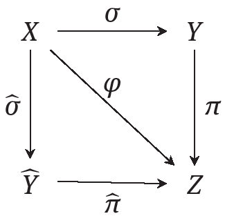
Then φ := π ∘ σ is a conic bundle, that is a fibre-type contraction whose generic fibre is a plane conic, and φ admits another factorisation φ:=π∘σ, where

is a ℙ¹-bundle, and σˆ:X→Yˆ is the blow-up with centre Sˆ:=σˆ(G)∩πˆ−1(A). Denote by Eˆ the exceptional divisor. Also, σˆ(G) and σˆ(Gˆ) are disjoint sections of πˆ,Nσˆ(G)/Yˆ ≅ 𝓞_Z(d − a) and Nσˆ(Gˆ)/Yˆ ≅ 𝓞_Z(a − d).

Now let C_Z be an irreducible curve in Z such that 𝓞_Z(1) ⋅ C_Z is minimal, let C_G ⊂ G and CGˆ⊂Gˆ be curves corresponding to C_Z, let F ⊂ E and Fˆ⊂Eˆ be fibres of, respectively, σ and σˆ. Then the cone of effective one-cycles NE(X) is closed and polyhedral, and is generated by the classes of

• F, Fˆ and CGˆ, if a = 0;

• F, Fˆ , C_G and CGˆ, if 0 < a < d;

• F, Fˆ and C_G, if a ≥ d.

All the relevant intersection numbers are collected in [5, Table 1], and one can see that

Furthermore, by [5, Remark 3.6], X is a Fano fourfold if and only if a ≤ i_Z − 1 and d − a ≤ i_Z − 1. By [5, Remark 3.7], the pairs (a, d) and (d − a, d) give rise to isomorphic fourfolds when d ≥ a, so we can assume that a > d or 0 ≤ a ≤ d/2.

Finally, by [5, Theorem 3.8], any Fano fourfold X of Picard number ρ_X = 3 which admits a prime divisor D with dim N₁(D, X) = 1 is isomorphic to one of the varieties X constructed above. Any such X, then, is given by a triplet (Z, a, d), where Z is a smooth Fano threefold with ρ_Z = 1 and

moreover |dH| contains a smooth surface. The inequalities (2.2) imply that the index of the Fano threefold Z cannot equal to 1. Note that the prime divisors G and Gˆ are isomorphic to Z, ρ_G = ρGˆ = 1, hence dimN₁(G, X) = dimN1(G^,X) = 1.

Remark 2.2

Further observations:

1. Since −K_X ⋅ F = 1, we have that the index of X is i_X = 1.

2. The classes of φ^∗H, Gˆ,E and the classes of φ^∗H, G, Eˆ are both a basis of N¹(X). Moreover,

for all α, β, γ ∈ ℝ, and

1. (iii) Under the conditions (2.2), Y and Yˆ are also Fano fourfolds by [11, Example 3.3(2)]. The cone Nef(Y) is generated by the classes of π^∗H and GˆY while Nef(Yˆ) is generated by the classes of πˆ∗Handσˆ(G). Note that the tautological line bundles 𝓞_Y (1) and OYˆ(1) are isomorphic, respectively, to the line bundles OY(GˆY)andOYˆ(σˆ(G)).

Remark 2.3

For any irreducible curve C ⊂ X, we set C^⊥ := {D ∈ N¹(X)|D ⋅ C = 0}. As X is smooth and Fano, the nef cone Nef(X) is closed and polyhedral, and is generated by finitely many extremal rays. A section of Nef(X) is

Moreover, τ = F^⊥ ∩ Nef(X), τˆ=Fˆ⊥ ∩ Nef(X), η = C_G^⊥ ∩ Nef(X), and ηˆ=CGˆ⊥ ∩ Nef(X). One can check that all the contractions are divisorial, apart from the contraction given by the ray R₁, which is always of fibre type and coincides with the conic bundle φ: X → Z, and the contraction given by the ray R₂ for a = 0, which is again of fibre type and corresponds to a morphism X → ℙ¹; the contractions of τ and τˆ are σ: X → Y and σˆ:X→Yˆ while the contractions of η and ηˆ send a divisor to a point, respectively G and Gˆ

In [15, Table § 12.1] we find the list of all smooth Fano threefolds with Picard number ρ_Z = 1. We are interested in those with index i _Z ≥ 2, and we collect all the relevant varieties in Table 1 for the reader’s convenience. The last two columns display, respectively, the base locus of the linear system |H|, and whether these varieties are rational (+) or not (−). We also include the dimension of the cohomology groups H⁰(T_Z) and H¹(T_Z) of the tangent sheaf T_Z. The references for h⁰(T_Z) are [20, Theorem 1.3] for Z₁, [18, Theorem 3.4] for Z₂, [19, Theorem 7.5] for Z₅, and [8, Theorem 1.1, Theorem 1.3] for Z₃, Z₄ and Z₆; see also [3, Theorem 3.1]. For similar results on the automorphism groups of smooth Fano threefolds with ρ_Z = 1, see [16, Theorem 1.1.2].

As for computing h¹(T_Z), by applying the Hirzebruch–Riemann–Roch theorem [13, Appendix A, Theorem 4.1] to the sheaves T_Z and ΩZ1 and the Nakano vanishing theorem [17, Theorem 4.2.3], we get

Lemma 2.4

For i = 2, . . . , 7, the line bundle 𝓞_Zi (d) is globally generated for all d ≥ 1, and 𝓞_Z1 (d) is globally generated for all d ≥ 2. Moreover, a general surface A ∈ |𝓞_Z1 (1)| is smooth.

Proof. Observe that, when i ≠ 1, 2, the ample generator 𝓞_Zi (1) of Pic(Z_i) corresponds to a hyperplane section in some projective space ℙ, thus it is very ample. This is clear for i = 3, 4, 6, 7, while it follows from [15, Theorem 3.2.5(v)] that 𝓞_Z5 (1) is the restriction to Z₅ of the very ample divisor on the Grassmannian Gr(2, 5) defining the Plücker embedding Gr(2, 5) ↪ ℙ⁹. Furthermore, 𝓞_Z2 (1) is globally generated since it is the pull-back of 𝓞_ℙ³ (1). Therefore, any positive multiple of the ample generator is globally generated.

As for Z₁, by [15, Proposition 2.4.1(i), Theorem 2.4.5(i)] we have that 𝓞_Z1 (2) is globally generated, while 𝓞_Z1 (1) has a unique simple base point. Moreover, 𝓞_Z1 (3) is very ample, see [16, Table 1], so that 𝓞_Z1 (d) is globally generated for all d ≥ 2. Nonetheless, by [15, Proposition 2.3.1], a general surface A in the linear system |𝓞_Z1 (1)| is smooth.

Corollary 2.5

For every Z_i, i = 1, . . . , 7, and for every choice of integers a, d satisfying(2.2), there exists a smooth Fano fourfoldXa,diof Picard number 3 constructed as in Remark 2.1.

Conversely, if X is a smooth Fano fourfold with ρ_X = 3 containing a prime divisor D with dim N₁(D, X) = 1, then X is isomorphic toXa,difor some (Z_i , a, d) as above. This gives rise to 28 families, see Table 2.

Proof. Assume that the integers a, d satisfy (2.2). This yields d ≤ 2i_Z − 2. Therefore, by Lemma 2.4, a general surface A ∈ |𝓞_Zi (d)| is smooth for every i = 1, . . . , 7, and so, given the triplet (Z_i , a, d), we can construct a Fano fourfold X := Xa,di of Picard number 3. Note that Xa,di contains a prime divisor G such that ρ_G = 1, hence dim N₁(G, X) = 1 (see Remark 2.1).

Conversely, by [5, Theorem 3.8], any Fano fourfold X of Picard number ρ_X = 3 which admits a prime divisor D with dim N₁(D, X) = 1 is isomorphic to one of the Xa,di

Lemma 3.1

Let W be a smooth variety, let ℙ(ε) be a ℙⁿ-bundle over W and letW˜be the blow-up of W along a subvariety V of codimension c. Then

Proof. By [7, Introduction 0.1] and quick computations.

Lemma 3.2

Let Z be a smooth Fano threefold with ρ_X = 1 and i_Z ≥ 2. Let A be a smooth surface in |𝓞_Z(d)|. Then all but the following Hodge numbers of A vanish:

• h ^0,0(A) = 1;

• h ^0,2(A) = 1, for d = i_Z;

• h ^0,2(A) = 5, for d = 4 and i_Z = 3 (i.e. Z is a smooth quadric threefold);

• h ^0,2(A) = d−13,for d = 5, 6 and i_Z = 4 (i.e Z ≅ ℙ³);

• h ^1,1(A) = 10 + 10 ⋅ h^0,2(A) − d(d − i_Z)²δ, where δ = H³.

Proof. We first carry out the computation for h^0,2(A). By the exact sequence

we have H²(𝓞_A)≅ H³(𝓞_Z(−d)). Moreover, h³(𝓞_Z(−d)) = 0 for d < i_Z, and h³(𝓞_Z(−d)) = 1 for d = i_Z by the Kodaira vanishing theorem. This concludes the case i_Z = 2. For i_Z = 3 we have 1 ≤ d ≤ 4 and h³(𝓞_Z(−4)) = h⁴(ℙ⁴, 𝓞_ℙ⁴ (−6)) = 5; for i_Z = 4 we have 1 ≤ d ≤ 6 and h³(𝓞_ℙ³ (−d)) = d−13 for d = 5, 6.

To compute h^1,1(A) we apply Noether’s formula χ_top(A) = 12χ(𝓞_A)− KA2 in [2, Remark I.14] to get

where δ = H³. Lastly, the vanishing of h^0,1(A) follows from the Lefschetz hyperplane theorem.

Proposition 3.3

([6], Lemma 3.2). Let W be a smooth projective variety, dim W = 4, and let α: W˜→Wbe the blow-up of W along a smooth irreducible surface V. Then

1. K W ˜ 4 = K W 4 − 3 ( K W | V ) 2 − 2 K V ⋅ K W | V + c 2 ( N V / W ) − K V 2 ;

2. K W ˜ 2 ⋅ c 2 ( W ˜ ) = K W 2 ⋅ c 2 ( W ) − 12 χ ( O V ) + 2 K V 2 − 2 K V ⋅ K W | V − 2 c 2 ( N V / W ) ;

3. χ ( O W ˜ ( − K W ˜ ) ) = χ ( O W ( − K W ) ) − χ ( O V ) − 1 2 ( ( K W | V ) 2 + K V ⋅ K W | V ) .

Proposition 3.4

Let W be a smooth projective variety of dimension 3, and ε a rank 2 vector bundle on W. Let β: ℙ(ε) → W be a ℙ¹-bundle over W. Then

1. (i) KP(E)4=−8KW⋅c1(E)2+32KW⋅c2(E)−8KW3;

2. (ii) KP(E)2⋅c2(P(E))=−2KW⋅c1(E)2+8KW⋅c2(E)−2KW3−4KW⋅c2(W);

3. (iii) χ(OP(E)(−KP(E)))=χ(OP(E))+6KW⋅c2(E)−12(3KW3+3KW⋅c1(E)2)−13KW⋅c2(W).

Proof. Let D be the divisor associated to det(ε), and let ξ be the divisor associated to 𝓞_ℙ(ε)(1). We have ∑i=02(−1)iβ∗ci(E)⋅ξ(2−i)=0, which yields

Then

• β ^∗(K_W + D)⁴ = 0;

• β ^∗(K_W + D)³ ⋅ ξ = (K_W + D)³;

• β ^∗(K_W + D)² ⋅ ξ² = β^∗(K_W + D)² ⋅ (β^∗D ⋅ ξ − β^∗c₂(ε)) = (K_W + D)² ⋅ D;

• β ^∗(K_W + D) ⋅ ξ³ = β^∗(K_W + D) ⋅ ξ ⋅ (β^∗D ⋅ ξ − β^∗c₂(ε)) = (K_W + D) ⋅ D² − (K_W + D) ⋅ c₂(ε);

• ξ ⁴ = (β^∗D ⋅ ξ − β^∗c₂(ε))² = D³ − 2D ⋅ c₂(ε).

We recall that K_ℙ(ε) = β^∗(K_W + D) − 2ξ, therefore

and we obtain (i).

To prove (ii), we need to compute c₂(ℙ(ε)). By [12, Example 3.2.11], we get

So, KP(E)2⋅c2(P(E)) = (β^∗(K_W + D) − 2ξ)² ⋅ (β^∗K_W ⋅ (β^∗D − 2ξ) + β^∗c₂(W)), which gives (ii). To get (iii), just apply (3.1).

Lemma 3.5

Let X be as in Corollary 2.5, and let δ = H³. Then

1. (i) KX4=8δiZ(a2+iZ2)−3dδ(a+iZ)2+2dδ(a+iZ)(d−iZ)+ad2δ−dδ(d−iZ)2,

2. (ii) KX2⋅c2(X)=84+2δiZ(a2+iZ2)−12h0,2(A)+2dδ(d−iZ)(a+d)−2ad2δ,

3. (iii) χ(OX(−KX))=8+32δiZ(a2+iZ2)−h0,2(A)−12dδ(a+iZ)(a−d+2iZ).

Proof. Recall that in the setting of Remark 2.1 we have ε = 𝓞_Z ⊕ 𝓞_Z(a), therefore det(ε) = 𝓞_Z(a), c₁(ε) = aH and c₂(ε) = 0. Since Z is a Fano threefold, the Riemann–Roch Theorem [13, Appendix A, Exercise 6.7] applied to the sheaf 𝓞_Z yields K_Z ⋅ c₂(Z) = −24. Moreover, the exact sequence

corresponds to

and so

1. (i) c₁(N_S/Y) = (a + d)H_|A under the natural isomorphism S ≅ A,

2. (ii) c₂(N_S/Y) = ad²δ.

Furthermore, it is not difficult to verify that K_Y|S = −(a + i_Z)H_|A, K_S = (d − i_Z)H_|A, thus

Finally, Proposition 3.3 yields

1. (i) KY4=8δiZ(a2+iZ2),

2. (ii) KY2⋅c2(Y)=2δiZ(a2+iZ2)+96,

3. (iii) χ(OY(−KY))=9+32δiZ(a2+iZ2),

and Proposition 3.4 gives the statement.

Remark 4.1

The construction of X, as in Remark 2.1, can be also done in families. Given a smooth family g: Z → B of Fano threefolds with Picard number 1 and index i _Z > 1, and given 𝓞_Z(ℋ) ∈ Pic(Z) such that the restriction 𝓞_Zb (ℋ_|Zb) to the fibre Z_b is the generator of Pic(Z_b) for all b ∈ B, it is possible to construct a smooth family of Fano fourfolds f:X→B˜ where B˜ is the open subset of PB((g∗OZ(dH))∨) which parametrises the smooth surfaces Ab∈|dH|Zb| | for all b ∈ B, so that the fibre of f over b˜∈B˜ is obtained from (Z_b, A_b) as in Remark 2.1.

Let us fix a smooth Fano threefold Z_i, i ∈ {1, . . . , 7}, and integers a, d satisfying (2.2), so that the varieties Xa,di of Corollary 2.5 are parametrised by couples (Z, A), with Z smooth and deformation equivalent to Z_i, and A ∈ |𝓞_Z(d)| is a smooth surface. In this section we use the notation X (Z, A) to denote the Fano fourfold given by the couple (Z, A).

Our first goal is to prove that if f : X → S is a smooth family of Fano varieties, and if there exists s₀ ∈ S such that its fibre X_s0 is isomorphic to X (Z_s0 , A_s0), then all the fibres X _s are isomorphic to Xa,di for some (Z_s , A_s), that is X_s ≅ X (Z_s , A_s).We are going to prove this by looking at the behaviour of the nef cone Nef(X_s), and the corresponding contractions, under the deformation f. Wiśniewski [24, Theorem 1] proved that, in the case of a smooth family of Fano varieties, the nef cone is locally constant. Moreover, generalised results in the setting of singular varieties were proved in [10] and [9].

Proposition 4.2

Let f : X → S be a smooth family of Fano varieties. Assume that there exists s₀ ∈ S such that the fibre X_s0is isomorphic toXa,diThen, any fibre X _s is one of the varieties of Corollary 2.5, and belongs to the same family of X_s0.

Proof. Step 1. We can assume that dim S = 1, and up to pull-back to the normalisation of S, we can assume that S is smooth. Since the fibres of a smooth family are all diffeomorphic, the second Betti number is constant on the fibres of f; moreover, for smooth Fano varieties, the second Betti number coincides with the rank of the Picard group. Therefore the fibres X _s are smooth Fano fourfolds of Picard number 3, for all s ∈ S.

Step 2. In the following we adopt an argument in [9] to show that the fibres of f have the same type of contractions.

By [9, Theorem 2.2], the monodromy action (see [22, Section 3]) of π₁(S, s) on H²(X_s , ℚ) is finite. As in the proof of [9, Theorem 2.7], we may take a finite étale cover g: V → S and the pull-back X_V = X ×_S V of f via g. The resulting family f_V: X_V → V, which is still a deformation of X_s0, now has trivial monodromy action on H²(X_t ,ℚ) for all t ∈ V. By [9, Theorem 2.12], the restriction map N¹(XX_V)→ N¹(X_t) is surjective for all t ∈ V.

As a consequence, the map

is an isomorphism for all t ∈ V, where N1(XV/V) is the real vector space of divisors with real coefficients, modulo numerical equivalence on the curves contracted by f_V.

Now, it follows from [23, Proposition 1.3] that every elementary contraction of a fibre X _t → W_t extends to a relative elementary contraction X_V → W, and conversely every relative elementary contraction XV→W) restricts to an elementary contraction XV→W) on every fibre. Therefore, [10, Theorem 4.1] implies that X_t1 → W_t1 is of fibre type (respectively divisorial, small) if and only if X_t2 → W_t2 of fibre type (respectively divisorial, small), for any t₁, t₂ ∈ V. By applying a similar technique as in the proof of [9, Theorem 2.7], we see that the contractions on the fibres are deformation equivalent.

Step 3. By Step 2 and Remark 2.3, all the fibres X _t of f_V have an elementary divisorial contraction sending a divisor to a point, which implies that they all contain a divisor G_t (the exceptional divisor of such a contraction) with dim N1(G_t, X_t) = 1. Then, by [5, Theorem 3.8], each fibre X _t is one of the varieties of Corollary 2.5, and since the numerical invariants in Table 2 are constant under deformation and are different amongst the families, we can conclude that each X_t is in the same family of X_s0.

Corollary 4.3

The varieties of Corollary 2.5 form 28 families of deformations. They are all distinct, and do not have common members.

The next step is to understand when the varieties of the same family are isomorphic.

Proposition 4.4

Let X = X(Z, A) and X' = X(Z' , A'). Then: X ≅ X' if and only if there exists an isomorphism ψ: Z → Z' such that ψ(A) = A'.

Proof. Assume first that X ≅ X'. Let φ and φ' be the conic bundles of Remark 2.1, and let ρ be the composition of φ' with the isomorphism X ≅ X'. The cones NE(φ) and NE(ρ), which are the convex cones in NE(X) generated by the curves contracted by φ and ρ, must coincide, since they are both fibre-type contractions of X, and X admits only one such contraction by Remark 2.3. Therefore, by [11, Proposition 1.14(b)], there exists a unique isomorphism ψ: Z → Z' which makes the following diagram commute:

Since the diagram commutes, the discriminant divisor Δ := {z ∈ Z | φ⁻¹(z) is singular} of φ maps via ψ onto the discriminant divisor Δ' of φ'. In fact Δ = A and Δ' = A', and we get the statement.

Conversely, if there exists and isomorphism ψ: Z → Z' such that ψ(A) = A', for smooth surfaces A, A' ∈ |𝓞_Z(d)|, then ψ lifts as an isomorphism between X(Z, A) and X(Z' , A').

Proposition 4.5

Let X = Xa,dibe a Fano fourfold as in Corollary 2.5. Then

Furthermore,

1. (i) if i = 1, . . . , 4, then equality holds;

2. (ii) if i = 7 and d = 1, 2, then X is rigid, that is h1(TX) = 0.

Proof. Inequality (4.1) follows from Propositions 4.2 and 4.4. As for (i), just observe that if i = 1, . . . , 4 then h⁰(T_Zi) = 0 (see Table 1), so that Aut(Z_i) is finite. Therefore, for a given deformation Z of Z_i there are at most finitely many different choices of A which yield isomorphic Fano fourfolds.

On the other hand, if i = 7 and d = 1, 2 we are in the case of hyperplanes and smooth quadrics in ℙ³. Since they are all projectively equivalent to each other, it follows that Xa,17andXa,27 are rigid. This gives (ii).

Proposition 5.1

Let X be as in Corollary 2.5. If H is globally generated, then so is −K_X.Otherwise, eitherX0,11and | − K_X| has a unique base point, or X ≅ X1,21and | − K _X| has two base points. In all cases, a general element of |− K_X| is smooth.

Proof. Step 1. Assume that H is globally generated. Then, by Remark 2.2(ii) and (5.1), we have

Therefore, |− K _X| has no base point and −K_X is globally generated.

Conversely, assume that H is not globally generated. Then Z = Z₁, and either a = 0 and d = 1, or a = 1 and d = 2. The linear system |H| has a unique simple base point P₀, while |2H| is free; moreover, recall that in Remark 2.1 we fixed a smooth surface A ∈ |dH|, which exists for Z = Z₁ and d = 1, 2 (see Table 1 and Lemma 2.4).

Step 2. Let Z = Z₁, a = 0 and d = 1; then, the smooth surface A ∈ |H| contains P₀, and the fibre T := φ⁻¹(P₀) over P₀ is equal to F₀ ∪ Fˆ0 where F₀ ⊂ E and Fˆ0⊂Eˆ are irreducible rational curves. Therefore

which is the point Q₀ ∈ Gˆ corresponding to P₀ under the isomorphism Gˆ ≅ Z. Now, observe that

and that, by computing the intersection number with the generators of NE(X), −2K_X − Gˆ is an ample divisor; see [5, Table 1]. This implies, by the Kodaira vanishing theorem, that h¹(𝓞_X(−K_X −Gˆ)) = 0, and the restriction

is surjective. Thus, Q₀ is a base point for |− K_X|, and Bs(|− K_X|) = {Q₀}. Note that in the class of 2φ^∗H + G +Gˆ, which is numerically equivalent to −K_X by (5.1), we can choose an effective divisor so that it is smooth at Q₀: fix an effective divisor D ≡ 2H so that P₀ ∉ D, and φ^∗D ∈ |2φ^∗H| does not contain Q₀. Therefore φ^∗D + G + Gˆ is smooth at Q₀, thus a general effective divisor in | − K _X| is smooth.

Step 3. The last case to consider is Z = Z₁, a = 1, d = 2. Let T be the fibre φ⁻¹(P₀) over P₀; then, similarly as above,

where {Q₁} = T ∩ G and {Q₂} = T ∩ Gˆ are the points corresponding to P₀ in G and Gˆ. Again, similarly as above,

the divisors −2K_X − G and −2K_X − Gˆ are ample, the restrictions

are surjective, thus Q₁ and Q₂ are base points for | − K_X|, and Bs(| − K_X|) = {Q₁, Q₂}.

We now show that a general effective divisor of | −K_X| is smooth. We have two possibilities: either A ∈ |2H| contains P₀ or it does not. If we assume the latter, then the divisor φ^∗A + G + Gˆ is smooth at Q₁ and Q₂. If we assume the former, then we can choose a divisor D ∈ |2H| such that P₀ ∉ D, which implies that the divisor φ^∗D + G + Gˆ ∈ | − K_X| is smooth at Q₁ and Q₂ (as in Step 2). Thus the statement holds.

Remark 7.1

The proof of Theorem 1.1 is a consequence of the results of the previous sections: Corollary 2.5 gives the 28 families, in Section 3 we compute the numerical invariants, Proposition 5.1 provides the results on the base locus of | − K_X|, and in Section 6 we discuss rationality.

Remark 7.2

As a final note, we can ask whether the varieties Xa,di of Theorem 1.1 appear as fibres of elementary fibre-type contractions, that is if they are "fibre-like". This property has been introduced and studied in [9], where the authors give two criteria for fibre-likeness, one necessary and one sufficient. As a consequence of [9, Corollary 3.9], by looking at the elementary contractions of Xa,di (see Remark 2.3) we see that, if a ≠ d/2 then Xa,di cannot be fibre-like.

References

[1] V. V. Batyrev, On the classification of toric Fano 4-folds. J. Math. Sci. (New York) 94 (1999), 1021–1050. MR1703904 Zbl 0929.1402410.1007/BF02367245Search in Google Scholar
[2] A. Beauville, Complex algebraic surfaces, volume 34 of London Mathematical Society Student Texts. Cambridge Univ. Press 1996. MR1406314 Zbl 0849.1401410.1017/CBO9780511623936Search in Google Scholar
[3] O. Benoist, Séparation et propriété de Deligne-Mumford des champs de modules d’intersections complètes lisses. J. Lond. Math. Soc. (2) 87 (2013), 138–156. MR3022710 Zbl 1375.1404910.1112/jlms/jds045Search in Google Scholar
[4] C. Casagrande, G. Codogni, A. Fanelli, The blow-up of ℙ4 at 8 points and its Fano model, via vector bundles on a del Pezzo surface. Rev. Mat. Complut. 32 (2019), 475–529. MR3942925 Zbl 1435.1404110.1007/s13163-018-0282-5Search in Google Scholar
[5] C. Casagrande, S. Druel, Locally unsplit families of rational curves of large anticanonical degree on Fano manifolds. Int. Math. Res. Not. no. 21 (2015), 10756–10800. MR3456027 Zbl 1342.1408810.1093/imrn/rnv011Search in Google Scholar
[6] C. Casagrande, E. A. Romano, Classification of Fano 4-folds with Lefschetz defect 3 and Picard number 5. J. Pure Appl. Algebra 226 (2022), Paper No. 106864, 13 pages. MR4297039 Zbl 1469.1408610.1016/j.jpaa.2021.106864Search in Google Scholar
[7] J. Cheah, The Hodge polynomial of the Fulton-MacPherson compactification of configuration spaces. Amer. J. Math. 118 (1996), 963–977. MR1408494 Zbl 0881.1400410.1353/ajm.1996.0040Search in Google Scholar
[8] X. Chen, X. Pan, D. Zhang, Automorphism and cohomology II: complete intersections. Preprint 2017, arXiv:1511.07906v6Search in Google Scholar
[9] G. Codogni, A. Fanelli, R. Svaldi, L. Tasin, Fano varieties in Mori fibre spaces. Int. Math. Res. Not. no. 7 (2016), 2026–2067. MR3509946 Zbl 1404.1405210.1093/imrn/rnv173Search in Google Scholar
[10] T. de Fernex, C. D. Hacon, Deformations of canonical pairs and Fano varieties. J. Reine Angew. Math. 651 (2011), 97–126. MR2774312 Zbl 1220.1402610.1515/crelle.2011.010Search in Google Scholar
[11] O. Debarre, Higher-dimensional algebraic geometry. Springer 2001. MR1841091 Zbl 0978.1400110.1007/978-1-4757-5406-3Search in Google Scholar
[12] W. Fulton, Intersection theory. Springer 1998. MR1644323 Zbl 0885.1402510.1007/978-1-4612-1700-8Search in Google Scholar
[13] R. Hartshorne, Algebraic geometry. Springer 1977. MR0463157 Zbl 0367.1400110.1007/978-1-4757-3849-0Search in Google Scholar
[14] B. Hassett, Y. Tschinkel, On stable rationality of Fano threefolds and del Pezzo fibrations. J. Reine Angew. Math. 751 (2019), 275–287. MR3956696 Zbl 0706293710.1515/crelle-2016-0058Search in Google Scholar
[15] V. A. Iskovskikh, Yu. G. Prokhorov, Algebraic geometry. V. Fano varieties, volume 47 of Encyclopaedia of Mathematical Sciences. Springer 1999. MR1668579 Zbl 0912.14013Search in Google Scholar
[16] A. G. Kuznetsov, Y. G. Prokhorov, C. A. Shramov, Hilbert schemes of lines and conics and automorphism groups of Fano threefolds. Jpn. J. Math. 13 (2018), 109–185. MR3776469 Zbl 1406.1403110.1007/s11537-017-1714-6Search in Google Scholar
[17] R. Lazarsfeld, Positivity in algebraic geometry. I. Springer 2004. MR2095471 Zbl 1093.1450110.1007/978-3-642-18808-4Search in Google Scholar
[18] R. Lyu, X. Pan, Remarks on automorphism and cohomology of finite cyclic coverings of projective spaces. Math. Res. Lett. 28 (2021), 785–822. MR4270273 Zbl 1466.1404910.4310/MRL.2021.v28.n3.a7Search in Google Scholar
[19] J. Piontkowski, A. Van de Ven, The automorphism group of linear sections of the Grassmannians G(1, N). Doc. Math. 4 (1999), 623–664. MR1719726 Zbl 0934.1403210.4171/dm/70Search in Google Scholar
[20] V. V. Przyjalkowski, K. A. Shramov, Automorphisms of weighted complete intersections. (Russian) Tr. Mat. Inst. Steklova 307 (2019), 217–229. English translation: Porc.Steklov Inst. Math. 307 (2019), 198–209. MR4070067 Zbl 1442.1415310.1134/S0081543819060129Search in Google Scholar
[21] T. Tsukioka, Classification of Fano manifolds containing a negative divisor isomorphic to projective space. Geom. Dedicata 123 (2006), 179–186. MR2299733 Zbl 1121.1403610.1007/s10711-006-9122-8Search in Google Scholar
[22] C. Voisin, Hodge theory and complex algebraic geometry. II. Cambridge Univ. Press 2003. MR1997577 Zbl 1032.1400210.1017/CBO9780511615177Search in Google Scholar
[23] J. A. Wiśniewski, On deformation of nef values. Duke Math. J. 64 (1991), 325–332. MR1136378 Zbl 0773.1400310.1215/S0012-7094-91-06415-XSearch in Google Scholar
[24] J. A. Wiśniewski, Rigidity of the Mori cone for Fano manifolds. Bull. Lond. Math. Soc. 41 (2009), 779–781. MR2557458 Zbl 1193.1402110.1112/blms/bdp025Search in Google Scholar
© 2023 Walter de Gruyter GmbH, Berlin/Boston
This work is licensed under the Creative Commons Attribution 4.0 International License.
Articles in the same Issue
- Frontmatter
- Pseudoholomorphic curves on the LCS-fication of contact manifolds
- Shellable tilings on relative simplicial complexes and their h-vectors
- On projections of free semialgebraic sets
- Filtrations of numerically flat Higgs bundles and curve semistable Higgs bundles on Calabi–Yau varieties
- Mean surface and volume particle tensors under L-restricted isotropy and associated ellipsoids
- Open books and embeddings of smooth and contact manifolds