Avoidance of the Lavrentiev gap for one-dimensional non-autonomous functionals with constraints
-
Carlo Mariconda


Abstract
Consider a positive functional
1 Introduction
We consider here a one-dimensional, vectorial functional of the Calculus of Variations
defined on the space of Sobolev functions
Of course, the best way to avoid the phenomenon is to make sure that the minimizers of F exist and are Lipschitz. This path was studied by Leonida Tonelli himself (see [35]); new results appeared in the last decades starting from the works of Francis Clarke and Richard Vinter [22] and Luigi Ambrosio, Oscar Ascenzi and Giuseppe Buttazzo [2] for coercive Lagrangians, under the very weak growth Condition (H) introduced by Francis Clarke in the seminal paper on the subject [21] and more recent works (e.g., [5, 6, 7, 14, 15, 24, 31]).
Conditions ensuring the non-occurrence of the phenomenon, other than Lipschitz regularity of the minimizers, were established by the pioneer paper by Giovanni Alberti and Francesco Serra Cassano in [1] for the autonomous case (i.e.,
for all
We shall refer as to
The main road to obtain the non-occurrence of the phenomenon (an exception is [23] where Maria Colombo and Rosario Mingione use some minimality properties to face multidimensional problem) is that to ensure that the sufficient conditions for the non-occurrence of the gap are satisfied for every admissible absolute continuous trajectory y. When the Lagrangian is non-autonomous, the Lavrentiev phenomenon may occur (though it is quite rare if L is coercive, see [37]), even with innocent looking Lagrangians, like in Manià’s problem (see [27])
It may happen that one may reach the infimum of the energy
F among the functions y satisfying the condition
An extension of [1, Theorem 2.4] for non-autonomous Lagrangians, without requiring further assumptions on the state or velocity variables of Λ, was recently provided by the author in [29]. The same paper establishes a sufficient condition, conjectured by Alberti in a personal communication, for the non-occurrence of the phenomenon with both endpoint conditions. The need of a different set of sufficient conditions to establish the non-occurrence of the Lavrentiev phenomenon between the one endpoint and the two endpoint problem was not considered before.
Two questions, strictly related one to each other, remained to be considered:
The approach by means of the techniques developed in [1], inherited in [29], for the two endpoint problem permits to consider just the case of real-valued Lagrangians. Now, being able to deal with extended-valued Lagrangians is not a purely aesthetical matter, since by adding suitable indicator functions (i.e., functions that take just the values 0 or
The first question was considered by Clarke in [21] and [28], for Lagrangians that satisfy an extra growth condition, though much weaker than the standard superlinearity: in this case the approximating sequence in energy may be chosen to be equi-Lipschitz. The second problem was considered by Arrigo Cellina, Alessandro Ferriero and Elsa Marchini in [16] for autonomous and just real-valued Lagrangians.
The present research addresses the two problems when the Lagrangian is infinite valued without involving any kind of growth condition.
The main core of the paper, Theorem 5.4 and Corollary 5.13, are a set of sufficient conditions for the non-occurrence of the Lavrentiev gap and phenomenon for Lagrangians that might take the value
We consider Lagrangians of the form
the effective domain
Λ is radially convex in v, i.e., for all
is convex, continuous and subdifferentiable (see Definition 2.5) up to
Radial convexity in v is a somewhat natural assumption in the Calculus of Variations: it was established in [5, 7] that if
The main achievement concerning the Lavrentiev phenomenon is Corollary 5.13, that for the sake of clarity we report here in a less general form.
Corollary 5.13.
In addition to the Basic Assumptions, Condition (S
Ψ is real-valued and bounded on the compact subsets of
For every compact subset
For every compact subset
Then:
The Lavrentiev phenomenon does not occur for the problem with one endpoint constraint
The Lavrentiev phenomenon does not occur for the problem with two endpoint constraints
the following condition holds:
Λ is bounded on
With the exception of the Radial Convexity Assumption, the sufficient conditions in Corollary 5.13 are less restrictive than those in [1, 29] for the unconstrained case and require some kind of local boundedness just inside the effective domain of L:
For problems with just one prescribed endpoint, differently from [1, Theorem 2.4] and [29, Corollary 3.7], we do neither impose that the effective domain of Λ contains a product of intervals nor the local boundedness of Λ on sets whose projection onto the velocity variable v contains a full neighborhood of the origin. Trying to avoid these conditions, following the approach of Alberti and Serra Cassano was performed successfully just for
We do not impose that Λ is bounded on all bounded subsets of
For problems with both prescribed endpoints, the requirement that
Once one assumes the Basic Assumptions and radial convexity in the last variable, we show with several examples that the failure of any of the other conditions of Corollary 5.13 may lead to the occurrence of the Lavrentiev phenomenon.
Corollary 5.13 relies on Theorem 5.4, which provides some sufficient conditions for the non-occurrence of the Lavrentiev gap at a specific admissible trajectory
The proof is constructive and allows to explicitly build a Lipschitz approximating sequence in the sense of Definition 3.1: an example of such a construction is fully described in Example 8.1.
The arguments of the proof have several sources of inspiration: Clarke’s formulation of a very slow growth condition based on the DBR type subgradient in [21] for problems without smoothness assumptions, [16] where a version of Theorem 5.4 is formulated for a real-valued, autonomous Lagrangian under some extra assumptions, e.g., convexity in v and continuity of L (we refer to [19] for a simplified proof of the main result), and [15] for how the authors deal with the extended-valued case in the more comfortable class of Lagrangians that satisfy a growth condition. All the authors exploit in different ways what we call here the DBR type subgradient: Lemma 6.2 shows that some fundamental estimates that concern this kind of subgradient, starting with those obtained in [21] and in [17], continue to hold in a more general setting assuming just boundedness assumptions on the Lagrangian (and not on its derivatives).
The conditions in Theorem 5.4 and Corollary 5.13 where both endpoint constraints
The paper is organized as follows. In Section 3 we recall some basic facts on the Calculus of Variations and on the Lavrentiev phenomenon. Section 4 is devoted to the definition of the topologies that are involved in the main results for the case of two endpoints and an extended-valued Lagrangian. In Section 5 we state the main results, Theorem 5.4 and Corollary 5.13, we discuss thoroughly some comparisons with respects to the results in the literature and give some examples on the importance of the validity of the various assumptions. Section 6 illustrates the fundamental tools of the proof; we thoroughly show the role of the DBR type subgradient and of the topological properties of the effective domain. Section 7 is devoted to the proof of Theorem 5.4. In Section 8 we provide some examples of occurrence of the Lavrentiev phenomenon when some of the assumptions of the main results are not satisfied. Finally, Section 9 draws some possible extensions. Some open questions are addressed in various parts of the paper.
2 Notation and basic assumptions on the Lagrangian
2.1 Notation
We introduce the main recurring notation:
The Euclidean norm in any
The closed ball of
If
For
2.2 Basic assumptions
Let
where
Basic Assumptions.
We assume the following conditions:
Δ is a subset of
2.3 Condition (S
+
)
We consider the following Condition (S
Condition (S${}^{+}$).
For every
a Lebesgue–Borel measurable nonnegative function
a nonnegative Borel function
a bounded variation function η on I with values in
such that, for a.e.
Remark 2.1.
Condition (S
whenever
for some nondecreasing function η.
Example 2.2.
Let
satisfies Condition (S
2.4 Structure assumptions on Λ
We recall here some important properties of the subgradient of a convex function, that will be used in the proof of the main results (see, for instance, [7, 36]).
Proposition 2.3 (Convex subgradient).
Let
The subset of such elements
The function
- (2.4)
In particular, P is the ordinate of the intersection of the tangent line
Remark 2.4.
While it is understood that the subgradient of a convex function exists within the interior of its effective domain, the existence of a subgradient of ϕ at 1, as stated in Proposition 2.3, is not inherently guaranteed and must therefore be explicitly assumed.
The following additional conditions on Λ will be assumed throughout the paper.
Definition 2.5 (Radial Convexity Assumption (RC)).
For a.e.
Moreover, the function
Definition 2.6 (Assumptions on
Dom
(
Λ
)
).
When Λ is extended valued, we assume the following conditions on its effective domain, defined by
The effective domain of Λ is a product:
(2.6)For every
(2.7)be the y-section of
(2.8)Thus if
Figure 1 illustrates an example of a domain that satisfies the conditions of Definition 2.6.
Remark 2.7.
Condition (2.5) in Definition 2.5 is somewhat natural in the Calculus of Variations. Indeed, it was established in [5, 7] that if
Remark 2.8.
Condition (2.6) is fulfilled if Λ is a product of functions of the form
If Λ is radially convex then (2.8) is fulfilled if
Notice, however, that the Structure Assumptions do not require
Let
An example of a subset
Let
is convex on
The function P plays a special role in the Calculus of Variations: under suitable assumptions it turns out that a minimizer
Definition 2.9 (Du Bois–Reymond (DBR) type subgradient).
Let
is a Du Bois–Reymond (DBR) type subgradient of Λ at
Remark 2.10.
It follows from Proposition 2.3 that
![Figure 2
Interpretation of
P
(
s
,
z
,
u
)
∈
∂
μ
[
Λ
(
s
,
z
,
u
μ
)
μ
]
μ
=
1
{P(s,z,u)\in\partial_{\mu}[\Lambda(s,z,\frac{u}{\mu})\mu]_{\mu=1}}
when
n
=
1
{n=1}
.](/document/doi/10.1515/acv-2023-0096/asset/graphic/j_acv-2023-0096_fig_0002.jpg)
Interpretation of
3 Lavrentiev gap at a function and Lavrentiev phenomenon
In this paper we consider different boundary data for the same integral functional.
3.1 The variational problems (
𝒫
Δ
,
𝒰
), (
𝒫
X
Δ
,
𝒰
), (
𝒫
X
,
Y
Δ
,
𝒰
)
We shall consider different variational problems associated to the functional F, with different endpoint conditions and state constraints.
Let
Free endpoints. We set
(${\mathcal{P}^{\Delta,\mathcal{U}}}$)One prescribed endpoint. If
(${\mathcal{P}_{X}^{\Delta,\mathcal{U}}}$)Two prescribed endpoints. If
(${\mathcal{P}_{X,Y}^{\Delta,\mathcal{U}}}$)
For the problems with one endpoint constraint, there is no privilege in considering the initial condition
3.2 Lavrentiev gap and phenomenon
Definition 3.1 (Lavrentiev gap at
y
∈
W
1
,
p
(
I
;
R
n
)
and Lavrentiev phenomenon).
Let
for all
We will refer to
Remark 3.2 (Gap and phenomenon).
AA
Once Condition (2) of Definition 3.1 is satisfied, in order to verify Condition (3) it is enough to check that
Indeed, Condition (2) and Fatou’s Lemma give
The non-occurrence of the Lavrentiev gap along a minimizing sequence (and in particular at every admissible
Concerning the Lavrentiev gap or phenomenon, there are several reasons to distinguish between problems with both endpoint conditions and those with just one endpoint condition. The main issue is that the phenomenon may occur in first case and not in the second, as shown by Example 3.3.
Example 3.3 (Manià, [27]).
Consider the problem of minimizing
Then
However, as it is noticed in [12], the situation changes drastically if one allows to vary the initial boundary condition along the sequence
The function
Then, for every
Therefore, no Lavrentiev phenomenon occurs for the variational problem
3.3 Examples of the occurrence of the gap or phenomenon
The Lavrentiev phenomenon may occur in the autonomous case for Lagrangians that take the value
Example 3.4 (Lavrentiev phenomenon with one endpoint constraint [19]).
Consider the autonomous Lagrangian
Notice that:
the effective domain of Λ is
In particular, Λ satisfies Condition (S) of Remark 2.1 and the Structure Assumptions (with
In the following examples, the Lavrentiev phenomenon occurs when the Lagrangian is a constant in its effective domain.
Example 3.5 (Lavrentiev phenomenon with one endpoint constraint).
Let
Notice that
The effective domain of Λ is
For all
Example 3.6 (Lavrentiev phenomenon with two endpoint constraints).
This example is inspired by one of Alberti (see [29]).
Consider, for
The set
The effective domain of Λ is
represented in Figure 4. Note that Λ satisfies the Structure Assumptions:
For all
For all
Clearly,
Note that it may not happen that
However, the change of variable
contradicting (3.4). Therefore
satisfies
4 Admissible topologies
This section may be skipped if Λ takes only finite values or for problems with just one end point condition.
When dealing with an extended-valued Lagrangian for problem (
4.1 The topology
τ
𝒲
induced by an equivalence relation
𝒲
in a metric space
We allow here a metric in metric spaces to take the value
Definition 4.1 (The “metric”
dist
W
).
Let
Proposition 4.2.
Let
Definition 4.3 (The topology
τ
W
).
Let
The topology
The functions
Proposition 4.4 (Inclusions between topologies and metrics).
Let
4.2 Admissible topologies in
ℝ
n
×
ℝ
n
In the main result of the paper we will consider topologies on
Definition 4.5 (Admissible topologies).
Let
We shall denote by
Remark 4.6.
It follows from Proposition 4.4 that
if
In particular, any topology
Example 4.7 (The topology of the y-sections).
Among the admissible topologies on
a set
are open in
The next result motivates the requirement that we consider just equivalence classes on
Proposition 4.8.
Let
4.3 Well-inside subsets of
D
Λ
We denote by
Definition 4.9 (The family
M
W
, the notation
⋐
W
).
Let
We shall denote by
Remark 4.10.
Let
The family of sets that are well-inside
Proposition 4.11.
Let
Remark 4.12.
It follows from Proposition 4.11 that
Observe that inequalities in (4.3) might be strict:
for instance, if
Example 4.13.
We consider here
If
Therefore
Analogously, if
Recalling that
For instance, if
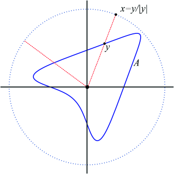
An example is depicted in Figure 5.
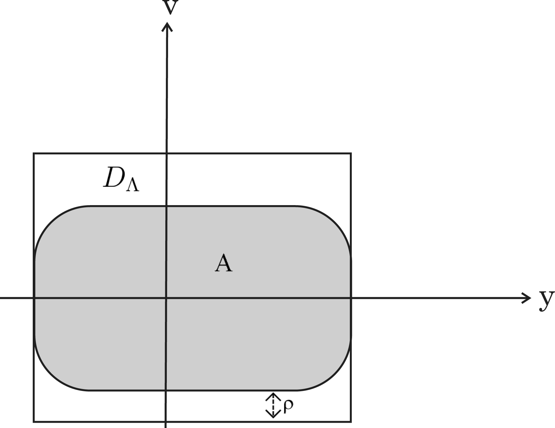
The set A is well-inside
5 Non-occurrence of the Lavrentiev gap and phenomenon
We present here the main results of the paper, on the non-occurrence of the gap or phenomenon. When the projection of the effective domain onto the velocity space
5.1 Non-occurrence of the Lavrentiev gap
We will require the boundedness of Λ on sets that “enclose” the origin, as does a sphere.
Definition 5.1 (Sets enclosing the origin).
We say that
There is
For all
A curve enclosing the origin in
Example 5.2.
A subset A of
5.1.1 Sufficient conditions for the non-occurrence of the gap
Theorem 5.4 makes use of the notion of admissible topology in
Definition 5.3 (
essinf
).
If u is a measurable function on I, we define
Theorem 5.4 (Non-occurrence of the Lavrentiev gap).
Let
There is
Ψ is bounded on
There is a subset
Then:
There is no Lavrentiev gap for (
There is no Lavrentiev gap for (
the following condition holds:
There is
In both cases the Lipschitz approximating sequence
Let us show how Theorem 5.4 may be of help.
Example 5.5.
Consider an autonomous Lagrangian of the form
where
Then Λ fulfills the Assumptions of Claim (1) in Theorem 5.4:
thus the Lavrentiev phenomenon does not occur for problem (
Example 5.6.
Consider an autonomous Lagrangian of the form
where
Then Λ fulfills the Assumptions of Claim (2) of Theorem 5.4, with
[28, Proposition 4.24, Theorem 5.1] require that Λ goes to infinity at the boundary of
5.1.2 On the assumptions of Theorem 5.4
We comment briefly the assumptions required in Theorem 5.4.
Remark 5.7.
Condition (S
Condition (
In Claim (2), Condition (a) is satisfied if
Since
Condition (
5.1.3 Choice of the equivalence relation
𝒲
The problem of the choice of a suitable equivalence relation on
Remark 5.8.
The choice of the suitable equivalence relation
Instead, Condition (
In order to verify the validity of the assumptions for the validity of Claim (2) in Theorem 5.4, one may proceed as follows:
Check whether
If the two conditions stated in (i) hold, check whether
If (ii) fails, try to find an intermediate equivalence relation
Example 5.9.
Suppose, for instance, that
Then
5.1.4 Counterexamples
Remark 5.10 (Counterexamples).
The Lavrentiev phenomenon may occur if some of the assumptions of Theorem 5.4 are not fulfilled:
The Lavrentiev phenomenon may occur, even for autonomous Lagrangians for the one endpoint problem (
Λ satisfies (
Condition (
When Λ is extended valued, the requirement that
We ignore whether the gap for constrained/extended-valued problems may occur if all the assumptions of Theorem 5.4 hold true, except the radial convexity one.
5.1.5 Comparison with known results in the literature
Theorem 5.4 is a step forward with respect to the results of the literature on Lavrentiev’s phenomenon.
Remark 5.11.
A first point of distinction is that the case with just one endpoint constraint has not been considered intentionally before as differing from the problem with both endpoint conditions, except in the author’s recent [29] (though without taking into account there the state constraint
Theorem 5.4 extends in several directions [16, Theorem 1] by Cellina, Ferriero and Marchini established for real-valued and continuous Lagrangians of the form
A particular case of Theorem 5.4 was formulated in [28, Theorem 5.1, Claim (2)], for a Lagrangian of the form
We study problem (
Assumption h
Finer topologies than the Euclidean one are not mentioned elsewhere.
The linear growth assumption from below (see ((G${{}_{\Lambda}}$)) in Section 5.2) is no more needed here.
We do not impose anymore, as in [28, Proposition 4.24] that, for all
We prove the convergence of the Lipschitz approximation not only – as in [28, Theorem 5.1] – in energy, but also in the
[29, Theorem 3.1] and [1, Theorem 2.4] do not consider the state constraint
Here, in addition to the conditions of [29, Theorem 3.1], we require the radial convexity of Λ in the last variable, a geometrical structure of the domain and, for the problem with two endpoint constraints, the topological condition that
The main improvement with respect to the existing literature, even in the unconstrained case, concerns the two endpoint problem where Condition (
For problem (
![Figure 7
The effective domain of an autonomous Lagrangian
Λ
(
s
,
y
,
v
)
=
L
(
y
,
v
)
{\Lambda(s,y,v)=L(y,v)}
(
n
=
1
{n=1}
,
𝒲
=
𝒲
e
=
ℝ
×
ℝ
{\mathcal{W}=\mathcal{W}_{e}={\mathbb{R}}\times{\mathbb{R}}}
so that the topology
τ
𝒲
{\tau_{\mathcal{W}}}
is the Euclidean one) and the validity of the assumptions of [29, Theorem 3.1] compared with those of Theorem 5.4 for problem (
𝒫
X
,
Y
ℝ
,
ℝ
{\mathcal{P}^{{\mathbb{R}},{\mathbb{R}}}_{X,Y}}
) (with
Δ
=
𝒰
=
ℝ
{\Delta=\mathcal{U}={\mathbb{R}}}
):
(a) Assumption (
B
y
,
Λ
+
{{\rm B}^{+}_{y,\Lambda}}
) in [29, Theorem 3.1] requires that there is a neighborhood
𝒪
y
{\mathcal{O}_{y}}
of
y
(
I
)
{y(I)}
such that, for all
r
>
0
{r>0}
, Λ is bounded on
𝒪
y
×
B
r
{\mathcal{O}_{y}\times B_{r}}
(the gray region); in particular
D
Λ
{D_{\Lambda}}
needs to contain the unbounded strip
𝒪
y
×
ℝ
{\mathcal{O}_{y}\times{\mathbb{R}}}
. (b) Hypotheses (
B
y
,
Λ
σ
{{\rm B}^{\sigma}_{y,\Lambda}}
)–(
B
y
,
Λ
⋐
𝒲
{{\rm B}^{\Subset_{\mathcal{W}}}_{y,\Lambda}}
) in Theorem 5.4 require that there are
a
y
<
0
,
b
y
>
0
{a_{y}<0,b_{y}>0}
such that Λ is bounded on
(
I
×
y
(
I
)
×
{
a
y
,
b
y
}
)
∩
Dom
(
Λ
)
{(I\times y(I)\times\{a_{y},b_{y}\})\cap\operatorname{Dom}(\Lambda)}
(strongly dotted lines) and there is
λ
y
>
essinf
{
|
y
′
(
s
)
|
:
s
∈
I
}
{{\lambda_{y}}>\operatorname{essinf}\{|y^{\prime}(s)|:s\in I\}}
such that Λ is bounded on the subsets of the form
I
×
A
{I\times A}
where
A
⊆
y
(
I
)
×
B
λ
y
{A\subseteq y(I)\times B_{\lambda_{y}}}
is relatively compact in
D
Λ
{D_{\Lambda}}
(e.g., the interior dotted region up to level
λ
y
{\lambda_{y}}
); it is also required that
Dom
(
Λ
)
{\operatorname{Dom}(\Lambda)}
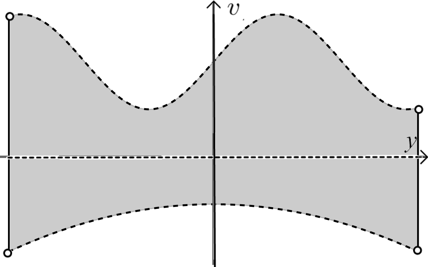
satisfies the assumptions of Definition 2.6.](/document/doi/10.1515/acv-2023-0096/asset/graphic/j_acv-2023-0096_fig_0008.png)
![Figure 7
The effective domain of an autonomous Lagrangian
Λ
(
s
,
y
,
v
)
=
L
(
y
,
v
)
{\Lambda(s,y,v)=L(y,v)}
(
n
=
1
{n=1}
,
𝒲
=
𝒲
e
=
ℝ
×
ℝ
{\mathcal{W}=\mathcal{W}_{e}={\mathbb{R}}\times{\mathbb{R}}}
so that the topology
τ
𝒲
{\tau_{\mathcal{W}}}
is the Euclidean one) and the validity of the assumptions of [29, Theorem 3.1] compared with those of Theorem 5.4 for problem (
𝒫
X
,
Y
ℝ
,
ℝ
{\mathcal{P}^{{\mathbb{R}},{\mathbb{R}}}_{X,Y}}
) (with
Δ
=
𝒰
=
ℝ
{\Delta=\mathcal{U}={\mathbb{R}}}
):
(a) Assumption (
B
y
,
Λ
+
{{\rm B}^{+}_{y,\Lambda}}
) in [29, Theorem 3.1] requires that there is a neighborhood
𝒪
y
{\mathcal{O}_{y}}
of
y
(
I
)
{y(I)}
such that, for all
r
>
0
{r>0}
, Λ is bounded on
𝒪
y
×
B
r
{\mathcal{O}_{y}\times B_{r}}
(the gray region); in particular
D
Λ
{D_{\Lambda}}
needs to contain the unbounded strip
𝒪
y
×
ℝ
{\mathcal{O}_{y}\times{\mathbb{R}}}
. (b) Hypotheses (
B
y
,
Λ
σ
{{\rm B}^{\sigma}_{y,\Lambda}}
)–(
B
y
,
Λ
⋐
𝒲
{{\rm B}^{\Subset_{\mathcal{W}}}_{y,\Lambda}}
) in Theorem 5.4 require that there are
a
y
<
0
,
b
y
>
0
{a_{y}<0,b_{y}>0}
such that Λ is bounded on
(
I
×
y
(
I
)
×
{
a
y
,
b
y
}
)
∩
Dom
(
Λ
)
{(I\times y(I)\times\{a_{y},b_{y}\})\cap\operatorname{Dom}(\Lambda)}
(strongly dotted lines) and there is
λ
y
>
essinf
{
|
y
′
(
s
)
|
:
s
∈
I
}
{{\lambda_{y}}>\operatorname{essinf}\{|y^{\prime}(s)|:s\in I\}}
such that Λ is bounded on the subsets of the form
I
×
A
{I\times A}
where
A
⊆
y
(
I
)
×
B
λ
y
{A\subseteq y(I)\times B_{\lambda_{y}}}
is relatively compact in
D
Λ
{D_{\Lambda}}
(e.g., the interior dotted region up to level
λ
y
{\lambda_{y}}
); it is also required that
Dom
(
Λ
)
{\operatorname{Dom}(\Lambda)}
satisfies the assumptions of Definition 2.6.](/document/doi/10.1515/acv-2023-0096/asset/graphic/j_acv-2023-0096_fig_0006.jpg)
The effective domain of an autonomous Lagrangian
5.1.6 The real-valued case
If Λ is real-valued, many of the assumptions of Theorem 5.4 are fulfilled and there is no need to worry about the topologies induced by an equivalence relation
Corollary 5.12 (Λ real-valued: Non-occurrence of the Lavrentiev gap).
Let
There is
Ψ is bounded on
There is a subset
Then:
There is no Lavrentiev gap for (
There is no Lavrentiev gap for (
There is
In both cases the approximating sequence for y in energy and norm is of Lipschitz reparametrizations of y.
5.2 Non-occurrence of the Lavrentiev phenomenon
As a consequence of Theorem 5.4, we obtain the following condition ensuring the non-occurrence of the Lavrentiev phenomenon.
Corollary 5.13 (Non-occurrence of the Lavrentiev phenomenon).
In addition to the Basic Assumptions, Condition (S
Ψ is real-valued and bounded on
There is
There is a subset
Then:
The Lavrentiev phenomenon does not occur for (
The Lavrentiev phenomenon does not occur for (
the following condition holds:
Λ is bounded on the subsets of the form
Proof.
We prove Point (2) of the corollary for the two endpoint problem (
Fix
The conclusion follows. ∎
Remark 5.14.
If
Remark 5.15.
Assume, that there are
and that
where
(see [29, Corollary 3.7]). We may assume that j is big enough in such a way that
and
so that
Remark 5.16.
When
for all
implicitly implying that
Λ is real-valued and bounded on bounded sets.
The proof of [29, Corollary 3.7] shows that, actually, Condition (S) required there might be replaced by the weaker Condition (S
The next Example 5.17 shows how it might be useful to consider finer topologies than the Euclidean one.
Example 5.17.
Let
Then
Many of the assumptions of Corollary 5.13 are satisfied for real-valued, continuous Lagrangians. Moreover, there is no need in this case to consider any admissible topology
Corollary 5.18 (Non-occurrence of the Lavrentiev phenomenon for (
P
X
,
Y
Δ
,
𝒰
)
– real-valued case).
Let Ψ and Λ be real-valued.
Suppose, in addition to the Basic Assumptions, Condition (S
Then the Lavrentiev phenomenon does not occur for (
Remark 5.19.
The claim and the assumptions of Corollary 5.18 almost overlap with those of [29, Corollary 3.7]. The extra Radial Convexity Assumption (RC) on Λ, required here, allows to deal with the constraint
Open Question 1.
Can one build an example of a Lagrangian and set Δ for which the Lavrentiev phenomenon occurs for the constrained problem
6 Preliminary results to the proof of the main result
In this section we formulate the fundamental tools of the proof of Theorem 5.4: Lemma 6.1 shows how radial convexity is used to lower the value of the energy at a given trajectory y by means of a DBR type subgradient (Definition 2.9); Lemma 6.2 illustrates how the conditions in Theorem 5.4 give some crucial bounds of the DBR subgradient. Finally, Lemma 6.5, needed just for the two endpoint problem (
6.1 Lowering the energy via convexity
The part of the proof of Theorem 5.4 concerning the estimate of the energy F along the built Lipschitz approximating sequence is based on the following inequalities, both consequences of the Radial Convexity Assumption (RC) that allow, given an admissible trajectory, to lower the value of the functional along one suitable reparametrization.
Lemma 6.1 (Estimates through DBR subgradients).
Assume the validity of the Structure Assumptions.
Let, for all
Proof.
Writing that
Multiplying both terms of the inequality by μ, we get
the conclusion follows. ∎
6.2 A crucial boundedness property on the DBR type subgradients
Let
Lemma 6.2 shows that, under some suitable local boundedness assumptions on Λ, these estimates become somewhat uniform as v varies, respectively, out of a ball and inside a ball of given radii. One difficulty is that
We refer to [9, Theorem 4.2] for the proof of Lemma 6.2.
Lemma 6.2 (Boundedness of the DBR type subgradients [8, Theorem 4.2]).
Suppose that Λ satisfies the Basic and the Structure Assumptions. Let
Assume that there exists a set
Then, for all
(6.2)Suppose that there exists
(6.3)
Remark 6.3.
Taking into account the geometric interpretation of the subdifferentials given in Remark 2.10:
Condition (i) in Lemma 6.2 has a geometrical interpretation: the intersection with the ordinate axis of the tangent lines to
(6.4)Similarly, Condition (ii) in Lemma 6.2 geometrically means that the intersection with the ordinate axis of the tangent lines to
(6.5)
6.3 Staying well-inside the domain with greater velocities
The following lemma, needed just for the problem with two endpoint conditions in the extended-valued case, explains the requirement in Claim (2) of Theorem 5.4 that
Lemma 6.5 (Staying well-inside the domain with greater velocity).
Let
There exist
Proof.
Let, for
Since, for a.e.
so that there is
Owing that
Since, for all
proving that Ω has the desired properties. ∎
7 Proof of Theorem 5.4
The proof of Theorem 5.4 follows the lines of the proof of [28, Theorem 5.1], which is more focused on the construction not only of a Lipschitz approximating sequence, but a equi-Lipschitz one, with a Lipschitz constant that is uniform with respect to the initial time and datum. We will emphasize the new points which are:
The non-occurrence of the gap for the problem with just one endpoint condition: the previous literature, except [29], did not emphasized a different set of conditions with respect to the two endpoint problem.
The new Condition (S
The presence of the function Ψ.
We build here an approximating sequence
As mentioned in the introduction, we build a sequence of reparametrizations
We fix
7.1 Change of variables and approximations
We shall often make use of the following change of variables formula for Lebesgue integrals.
Proposition 7.1 (Change of variables for Lebesgue integrals [34]).
Let
The following approximation argument will be used in the sequel; we refer to [18] for a proof.
Lemma 7.2.
Let
for all ν,
the sequence of Lipschitz constants
for a.e.
Then
7.2 Proof of Claim (2) of Theorem 5.4
Proof.
We begin by proving the more challenging Claim (2). We consider several steps.
(i) Definition of
We may assume that
(ii).
For every
Indeed,
The purpose of Steps (iii)– (vi) is that to define the set
(iii) Definition of
and
For every
It follows from (7.3) that
(iv) Choice of
As pointed out in Remark 6.4, Hypothesis (
(v) Choice of
We may thus select a measurable subset
(vi) Choice of
where
(vii) Choice of
Let
We further choose
where we denote by
and, recalling from (7.2) that
From now on we set
(viii) The change of variable
Notice that
Therefore the image of
(ix).
Set, for all
Then
(x)
The fact that
Notice that, since
(xi). The following estimate holds:
Indeed,
in virtue of Step (v) and (7.7).
In Steps (xii)–(xvii) we compare
(xii).
For all
Indeed, let
Since
inequality (7.15) then follows immediately from the fact that
(xiii). This step, needed just for the problem with two endpoint conditions (
Indeed, since
By applying Lemma 6.1, recalling that
whence (7.16).
(xiv).
The following estimate of
Indeed, we have
Taking into account (7.12), the change of variables
where we set
Estimate of
(7.20)
Estimate of
(7.21)whence
(7.22)
Therefore, (7.17) follows now immediately from (7.18), (7.19), (7.20) and (7.22).
(xv) Choice of
(xvi). The following estimate holds:
Indeed, by adding and subtracting of both
where
and
It follows from (7.23) that
Condition (S
From [4, Lemma 2.10] we have
where
which, together with (7.25), give (7.24).
(xvii) Final estimate of
It follows from (7.10) that
(xviii) Proof of the convergence of
(7.27)
where in the above
Since
(7.28)as a consequence of Lemma 7.2 since, from Step (xi),
Recall that
(7.29)Since
It follows from (7.29) that
(7.30)In
(7.31)
Since
It follows from (7.31) that
(7.32)
We deduce from (7.27), together with (7.28), (7.30) and (7.32) that
7.3 Proof of Claim (1) of Theorem 5.4
Proof.
The proof is similar than that of Claim (2), from which we actually skip many steps. We just summarize the main issues. A self contained in the particular case where
Referring to the proof of Claim (2) of Theorem 5.4, we do not need here to build the sets Υ, Ω and
We keep Steps (i) and (ii).
We skip Steps (iii)–(vi). We do not need to choose
In Step (vii) we set
We then modify as follows the steps of the proof of Claim (2):
(viii’) The change of variable
As in the proof of Claim (2),
(ix’).
Set, for all
The new fact is that now
We now proceed as in the proof of Claim (2) up to Step (xii), skipping Step (xiii), not needed here. We need a little more care in the estimates in the last steps, the change of variable being now
(xiv’). Condition (7.17) becomes now
Similarly, all the integrals where
(xvi’). We choose
(xvii’). Inequality (7.26) is now
(xviii’). Similar arguments apply to the proof of the convergence of
(7.37)
The proof is complete. ∎
Remark 7.3.
In the case of a final endpoint constraint, instead of the initial one, Claim (1) of Theorem 5.4 may be obtained by slightly modifying Step (viii’) of the proof: indeed, it is enough to define
Remark 7.4.
For problems with one endpoint constraint, or when Λ is real-valued, the proof of Theorem 5.4 is constructive. Indeed,
for problems with one endpoint condition, the approximating functions
It is then enough to define
8 Examples
In Example 3.6, we showed directly that the Lavrentiev gap at a minimizer
Example 8.1 (A constructive method).
Consider the Lagrangian considered in Example 3.6. We already noticed that Λ satisfies the Basic and Structure Assumptions. Moreover, Λ is equal to 0 and thus bounded on every subset of
Following Step (viii’) of the proof of Theorem 5.4,
the change of variable
Therefore we have
Notice that
The inverse
Then
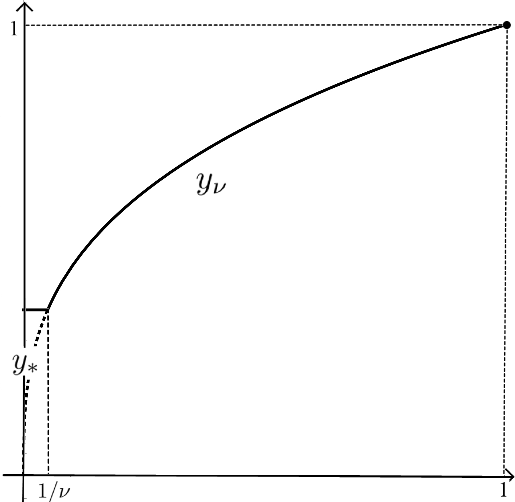
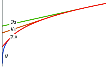
Figure 8 depicts the graphs of some of these approximations for some values of ν.
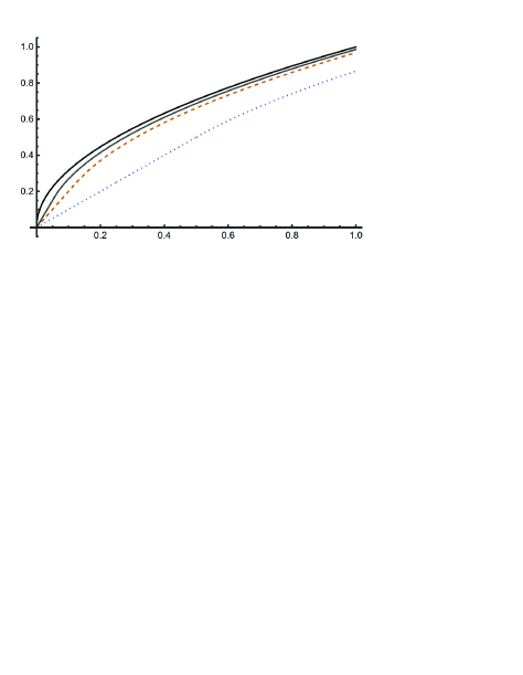
The absolutely continuous function
Notice that
so that
and
as
as
In the next example we show how the constructive method in the proof of Theorem 5.4 may lead to a sequence
Example 8.2.
Consider Manià’s example, where the Lagrangian
and let
and
This raises the following:
Open Question 2.
Can the non-occurrence of the gap with the endpoint constraint
We show here how, in the proof of Theorem 5.4, the violation of the integrability of
Fix
Thus we obtain, for all
Notice that, as expected,
The inverse
Following Step (ix) we therefore define, for all
Notice that of course
Lipschitzianity. For all
Convergence in
Failure of the convergence in energy. We have
for some positive constant α. Thus
The functions
9 Further developments and questions
Remark 9.1.
The proof of Theorem 5.4 relies on the fact that, for some
(9.1)and there is
(9.2)
Open Question 3.
Properties (9.1)–(9.2) are named Growth Condition (M
The conclusions of the paper may be easily extended to Lagrangians of the form
The proof of Theorem 5.4 shows that, in the boundedness conditions for Ψ and Λ one can replace
The main results can be generalized easily to an optimal control problem of the form
subject to
(D)where
the control
the control set
In this context the Lavrentiev gap does not occur at
The proof can be obtained following the lines of the proof of Theorem 5.4 with the obvious modifications (see the proof of [28, Theorem 5.1]); the details, in the case where
Dedicated to Francis Clarke on his 75th birthday
Funding statement: This research received partial funding from the University of Padua under the grant SID 2018 “Controllability, stabilizability and infimum gaps for control systems”, protocol BIRD 187147. Additionally, it was supported by the European Union – NextGenerationEU under the National Recovery and Resilience Plan (NRRP), Mission 4 Component 2 Investment 1.1 – Call PRIN 2022 No. 104 of February 2, 2022 by the Italian Ministry of University and Research; Project 2022238YY5 (subject area: PE – Physical Sciences and Engineering) titled “Optimal control problems: Analysis, approximation and applications”. Furthermore, this project was successfully completed with contributions from the UMI Group TAA “Approximation Theory and Applications”.
Acknowledgements
I am deeply thankful to Piernicola Bettiol and Raphaël Cerf for their gracious hospitality during my visits to the Université de Bretagne Occidentale (Brest) and the École Normale Supérieure de Paris, respectively. The welcoming and intellectually stimulating environments at these institutions greatly enhanced my ability to work on and refine this paper. My gratitude also extends to Pierre Bousquet and Giulia Treu for their insightful questions and keen attention throughout the preparation of our upcoming survey on our recent findings regarding the Lavrentiev phenomenon. I owe a special thank you to Giuseppe De Marco for the valuable discussions on the admissible topologies addressed in Section 4 and to the referees for their thoughtful remarks and suggestions.
References
[1] G. Alberti and F. Serra Cassano, Non-occurrence of gap for one-dimensional autonomous functionals, Calculus of Variations, Homogenization and Continuum Mechanics (Marseille 1993), Ser. Adv. Math. Appl. Sci. 18, World Scientific, River Edge (1994), 1–17. Search in Google Scholar
[2] L. Ambrosio, O. Ascenzi and G. Buttazzo, Lipschitz regularity for minimizers of integral functionals with highly discontinuous integrands, J. Math. Anal. Appl. 142 (1989), no. 2, 301–316. 10.1016/0022-247X(89)90001-2Search in Google Scholar
[3] J. M. Ball and V. J. Mizel, One-dimensional variational problems whose minimizers do not satisfy the Euler–Lagrange equation, Arch. Ration. Mech. Anal. 90 (1985), no. 4, 325–388. 10.1007/BF00276295Search in Google Scholar
[4] J. Bernis, P. Bettiol and C. Mariconda, Value function for nonautonomous problems in the calculus of variations, Math. Control Relat. Fields (2024), to appear. 10.3934/mcrf.2024045Search in Google Scholar
[5] P. Bettiol and C. Mariconda, A new variational inequality in the calculus of variations and Lipschitz regularity of minimizers, J. Differential Equations 268 (2020), no. 5, 2332–2367. 10.1016/j.jde.2019.09.011Search in Google Scholar
[6] P. Bettiol and C. Mariconda, Regularity and necessary conditions for a Bolza optimal control problem, J. Math. Anal. Appl. 489 (2020), no. 1, Article ID 124123. 10.1016/j.jmaa.2020.124123Search in Google Scholar
[7] P. Bettiol and C. Mariconda, A Du Bois–Reymond convex inclusion for nonautonomous problems of the calculus of variations and regularity of minimizers, Appl. Math. Optim. 83 (2021), no. 3, 2083–2107. 10.1007/s00245-019-09620-ySearch in Google Scholar
[8] P. Bettiol and C. Mariconda, Uniform boundedness for the optimal controls of a discontinuous, non-convex Bolza problem, ESAIM Control Optim. Calc. Var. 29 (2023), Paper No. 12. 10.1051/cocv/2022079Search in Google Scholar
[9] P. Bettiol, G. De Marco and C. Mariconda, A useful subdifferential in the Calculus of Variations, J. Nonlinear Anal., to appear. Search in Google Scholar
[10] P. Bousquet, C. Mariconda and G. Treu, On the Lavrentiev phenomenon for multiple integral scalar variational problems, J. Funct. Anal. 266 (2014), no. 9, 5921–5954. 10.1016/j.jfa.2013.12.020Search in Google Scholar
[11] G. Buttazzo and M. Belloni, A survey on old and recent results about the gap phenomenon in the calculus of variations, Recent Developments in Well-Posed Variational Problems, Math. Appl. 331, Kluwer Academic, Dordrecht (1995), 1–27. 10.1007/978-94-015-8472-2_1Search in Google Scholar
[12] G. Buttazzo, M. Giaquinta and S. Hildebrandt, One-Dimensional Variational Problems, Oxford Lecture Ser. Math. Appl. 15, Oxford University, New York, 1998. 10.1093/oso/9780198504658.001.0001Search in Google Scholar
[13] G. Buttazzo and V. J. Mizel, Interpretation of the Lavrentiev phenomenon by relaxation, J. Funct. Anal. 110 (1992), no. 2, 434–460. 10.1016/0022-1236(92)90038-KSearch in Google Scholar
[14] A. Cellina, The classical problem of the calculus of variations in the autonomous case: Relaxation and Lipschitzianity of solutions, Trans. Amer. Math. Soc. 356 (2004), no. 1, 415–426. 10.1090/S0002-9947-03-03347-6Search in Google Scholar
[15] A. Cellina and A. Ferriero, Existence of Lipschitzian solutions to the classical problem of the calculus of variations in the autonomous case, Ann. Inst. H. Poincaré C Anal. Non Linéaire 20 (2003), no. 6, 911–919. 10.1016/s0294-1449(03)00010-6Search in Google Scholar
[16] A. Cellina, A. Ferriero and E. M. Marchini, Reparametrizations and approximate values of integrals of the calculus of variations, J. Differential Equations 193 (2003), no. 2, 374–384. 10.1016/S0022-0396(02)00176-6Search in Google Scholar
[17] A. Cellina, G. Treu and S. Zagatti, On the minimum problem for a class of non-coercive functionals, J. Differential Equations 127 (1996), no. 1, 225–262. 10.1006/jdeq.1996.0069Search in Google Scholar
[18] R. Cerf and C. Mariconda, Occurrence of gap for one-dimensional scalar autonomous functionals with one end point condition, preprint (2022), https://arxiv.org/abs/2209.03820; to appear in Ann. Sc. Norm. Super. Pisa Cl. Sci. (5). 10.2422/2036-2145.202209_007Search in Google Scholar
[19] R. Cerf and C. Mariconda, The Lavrentiev phenomenon, preprint (2024), https://arxiv.org/abs/2404.02901; to appear in Amer. Math. Monthly. Search in Google Scholar
[20] F. Clarke, Functional Analysis, Calculus of Variations and Optimal Control, Grad. Texts in Math. 264, Springer, London, 2013. 10.1007/978-1-4471-4820-3Search in Google Scholar
[21] F. H. Clarke, An indirect method in the calculus of variations, Trans. Amer. Math. Soc. 336 (1993), no. 2, 655–673. 10.1090/S0002-9947-1993-1118823-3Search in Google Scholar
[22] F. H. Clarke and R. B. Vinter, Regularity properties of solutions to the basic problem in the calculus of variations, Trans. Amer. Math. Soc. 289 (1985), no. 1, 73–98. 10.1090/S0002-9947-1985-0779053-3Search in Google Scholar
[23] M. Colombo and G. Mingione, Bounded minimisers of double phase variational integrals, Arch. Ration. Mech. Anal. 218 (2015), no. 1, 219–273. 10.1007/s00205-015-0859-9Search in Google Scholar
[24] G. Dal Maso and H. Frankowska, Autonomous integral functionals with discontinuous nonconvex integrands: Lipschitz regularity of minimizers, DuBois–Reymond necessary conditions, and Hamilton-Jacobi equations, Appl. Math. Optim. 48 (2003), no. 1, 39–66. 10.1007/s00245-003-0768-4Search in Google Scholar
[25] W. B. Gordon, A minimizing property of Keplerian orbits, Amer. J. Math. 99 (1977), no. 5, 961–971. 10.2307/2373993Search in Google Scholar
[26] J. Malý and W. P. Ziemer, Fine Regularity of Solutions of Elliptic Partial Differential Equations, Math. Surveys Monogr. 51, American Mathematical Society, Providence, 1997. 10.1090/surv/051Search in Google Scholar
[27] B. Manià, Sopra un esempio di Lavrentieff, Boll. Unione Mat. Ital. 13 (1934), 147–153. 10.1007/BF02413436Search in Google Scholar
[28] C. Mariconda, Equi-Lipschitz minimizing trajectories for non coercive, discontinuous, non convex Bolza controlled-linear optimal control problems, Trans. Amer. Math. Soc. Ser. B 8 (2021), 899–947. 10.1090/btran/80Search in Google Scholar
[29] C. Mariconda, Non-occurrence of gap for one-dimensional non-autonomous functionals, Calc. Var. Partial Differential Equations 62 (2023), no. 2, Paper No. 55. 10.1007/s00526-022-02391-5Search in Google Scholar
[30] C. Mariconda, Non-occurrence of the Lavrentiev gap for a Bolza type optimal control problem with state constraints and no end cost, Commun. Optim. Theory 12 (2023), 1–18. Search in Google Scholar
[31] C. Mariconda and G. Treu, Lipschitz regularity of the minimizers of autonomous integral functionals with discontinuous non-convex integrands of slow growth, Calc. Var. Partial Differential Equations 29 (2007), no. 1, 99–117. 10.1007/s00526-006-0059-4Search in Google Scholar
[32] C. Mariconda and G. Treu, Non-occurrence of a gap between bounded and Sobolev functions for a class of nonconvex Lagrangians, J. Convex Anal. 27 (2020), no. 4, 1247–1259. Search in Google Scholar
[33] C. Mariconda and G. Treu, Non-occurrence of the Lavrentiev phenomenon for a class of convex nonautonomous Lagrangians, Open Math. 18 (2020), no. 1, 1–9. 10.1515/math-2020-0001Search in Google Scholar
[34] J. Serrin and D. E. Varberg, A general chain rule for derivatives and the change of variables formula for the Lebesgue integral, Amer. Math. Monthly 76 (1969), 514–520. 10.1080/00029890.1969.12000249Search in Google Scholar
[35] L. Tonelli, Fondamenti di calcolo delle variazioni. I., N. Zanichelli, Bologna, 1922. Search in Google Scholar
[36] R. Vinter, Optimal Control, Mod. Birkhäuser Class., Birkhäuser, Boston, 2000. Search in Google Scholar
[37] A. J. Zaslavski, Nonoccurrence of the Lavrentiev phenomenon for many optimal control problems, SIAM J. Control Optim. 45 (2006), no. 3, 1116–1146. 10.1137/050640370Search in Google Scholar
© 2024 Walter de Gruyter GmbH, Berlin/Boston
This work is licensed under the Creative Commons Attribution 4.0 International License.
Articles in the same Issue
- Frontmatter
- Γ-convergence analysis of the nonlinear self-energy induced by edge dislocations in semi-discrete and discrete models in two dimensions
- Characterization of the subdifferential and minimizers for the anisotropic p-capacity
- The best approximation of a given function in L 2-norm by Lipschitz functions with gradient constraint
- Quantitative C 1-stability of spheres in rank one symmetric spaces of non-compact type
- The Yang–Mills–Higgs functional on complex line bundles: Asymptotics for critical points
- A sub-Riemannian maximum modulus theorem
- The least gradient problem with Dirichlet and Neumann boundary conditions
- The 2+1-convex hull of a~finite set
- Non-local BV functions and a denoising model with L 1 fidelity
- Avoidance of the Lavrentiev gap for one-dimensional non-autonomous functionals with constraints